1. Introduction
Understanding user mobility from trajectory data has received considerable attention among users and developers. As a central component of understanding user mobility [
1], the identification of transportation modes used by people can provide rich information for some tasks and utilized in many applications. First, the information of transportation modes used by users is applicable to the travel behavior research field [
2,
3]. Travel behavior is concerned with the transportation people take, the routes they choose, and so on. According to the user’s daily transportation mode, we can discover the user’s behavior, and thus carry out personalized recommendations and provide intelligent services. For example, the system may recommend residential or transportation services if somebody is traveling on a train. Second, it is a significant part of transportation planning [
4] and traffic management, where transportation mode selection greatly influences transportation planning. In the past, this type of information was usually collected traditionally through questionnaires or telephone surveys, which were always expensive, inconvenient, time-consuming and inaccurate. However, if we can automatically identify the transportation modes accurately, it will also be a great convenience to people who trace their outdoor activity. Third, transportation mode identification can also serve other applications, such as GPS trajectories sharing applications [
5], sports products and intelligent surveillance systems. For example, in trajectory sharing applications, the information on transportation modes could ensure greater meaningful sharing and assist it in calculating the number of calories burnt.
Many studies in the previous decade have focused on inferring transportation modes from trajectory data by using machine learning methods to identify transportation modes from GPS or accelerometer data, which have achieved great results. However, there are still several limitations in these studies. First, many studies promote performance mainly through two ways: (1) The use of more sensors (gyroscope, and rotation vector) or more accurate sensors (professional device) to collect trajectory data [
6,
7,
8,
9], which improves performance, as more accurate data means more difference between transportation modes. However, it is difficult for people to carry many sensors around in their daily lives, therefore, it is not a realistic option for most people; (2) The use Geographic Information System information (GIS) to create more discriminative features [
10,
11]. However, it is not always easy to access GIS information and is not suitable for all cities. Second, almost all studies use traditional machine learning algorithms such as Decision Tree, K-Nearest Neighbor and Support Vector Machines [
6,
7,
10,
11,
12,
13,
14,
15,
16,
17]. However, these methods were found to be worse than ensemble methods, not only in terms of accuracy but also model robustness [
18,
19,
20,
21].
Given the above limitations, we propose a method to infer hybrid transportation modes only from GPS data to achieve a good performance in a real life trajectory dataset collected by Microsoft Geolife Project [
14,
15]. The unique contributions of this research effort are as follows:
- (1)
We used the statistics method [
22] to generate some discriminative global features and then extracted local features from sub-trajectories after trajectory segmentation [
23]. These features were then combined into a feature vector fed into the classification stage, which proved more robust than other used features and helped improve classification accuracy.
- (2)
We used tree-based ensemble models to classify the transportation modes, which proved to outperform other traditional methods (K-Nearest Neighbor, Support Vector Machines, and Decision Tree) in many evaluations.
- (3)
We extracted a lot of features, then used tree-based ensemble models to obtain feature importance, and then reduced the model complexity by removing the unimportant features, which our performance was better than the Principal Component Analysis (PCA) method.
- (4)
Using our approach, we could identify six different transportation modes including walking, cycling, driving a car, taking a train and taking subway. The highest accuracy was 90.77% and was obtained only through GPS data.
The rest of our paper is organized as follows. The relevant literature is reviewed in the following section, before a brief introduction on how the classification models were developed. Related experiments of the study and discussion are then presented before our conclusions on the study.
2. Related Work
This section provides a summary of related work in the area of transportation mode identification, with almost all studies taking advantage of machine learning methods such as Decision tree [
7,
13,
14,
15,
24,
25], K-Nearest Neighbor [
13], Support vector machines [
12,
13,
14,
17,
23], Artificial neural networks [
26,
27], Random forest [
13,
24], Fuzzy systems [
28,
29] and hidden Markov models [
25,
30,
31]. Among them, the Decision Tree and SVM methods were identified as the best when compared to other methods [
13,
14,
16]. Other than these machine learning methods, statistical methods were also applied, such as Random Subspace Method [
32]. In addition, Endo et al. [
33] proposed a method using a deep neural network (DNN) by converting the raw trajectory data structure into image data structure.
Many studies wanting to improve model performance primarily depend on the following methods, such as extracting more discriminative features from GPS trajectories. For example, Zheng et al. [
14] used common statistical features such as mean velocity, expectation of velocity, expectation of velocity, top three velocities and top three accelerations to identify four different transportation modes (Bike, Bus, Car, Walk). Zheng et al. [
15] further introduced more advanced features including the heading change rate (HCR), the stop rate (SR), and the velocity change rate (VCR), which achieved a more accurate performance. Additionally, using extra sensors such as accelerometers, gyroscopes, rotation vectors to collect more accurate data provides greater detailed information between the different transportation modes. For example, Nick [
16], Jahangiri [
12,
13], and Widhalm [
31] used mobile phone sensors to collect accelerometer data of different transportation modes, which achieved a better performance than only using GPS data. Other examples in References [
8,
9] used body temperature, heart rate, light intensity obtained from other sensors as features, and were able to build a model for predicting user activities including walking, running, rowing and cycling. Furthermore, GIS data can be used to create more distinguished features, as detailed in References [
24,
28]. For example, Stenneth [
24] derived the relevant features relating to transportation network information and improved the classification effectiveness of detection by 17% in comparison with only GPS data, which included real time bus locations, spatial rail and bus stop information.
Table 1 summarizes the related work in the field of transportation modes identification.
It appears that these methods have at least one of the following constraints. Firstly, these methods are overly dependent on using multiple sensors to collect more accurate data or matching GIS information to generate more discriminative features; however, often only the GPS data are available as it is difficult to store the data from the different sensors at specific times, and it was not possible to access GIS data in many cities. Therefore, this study only used GPS data, which can also achieve high accuracy. Although Gonzalez [
26,
27] achieved 91.23% accuracy, only three transportation modes were identified. Secondly, most of these methods need to consider feature scaling as the values of raw data vary widely. In some machine learning algorithms, objective functions will not work properly without normalization; however, the tree-based ensemble method does not require feature scaling as these methods are invariant to monotonic transformations of individual features so feature scaling will not change anything in these methods. Thirdly, most of these methods do not use feature selection methods as some redundant and unimportant features are useless, which also adds the model complexity. Some studies use the PCA method for feature reduction; however, we used the tree-based ensemble methods to conduct feature selection, which performed better than the PCA method. Fourthly, most studies use single stronger classifiers (Decision, Tree, K-Nearest Neighbor, and Support Vector Machines) to identify transportation modes, but ensemble methods have been found to do better than these classifiers as ensemble methods are a combination set of weak learners, which are superior to a single stronger learner, and have been widely proven in many machine learning challenges [
18,
19,
20]. Although some of them also use the random forest method, our method is different from these studies as we use other ensemble methods including GBDT [
34] and XGBoost [
19] besides the RF method. Furthermore, we used the ensemble method to conduct feature selection, which significantly differs from other recent work.
In this paper, we propose an approach using a tree-based ensemble method to infer hybrid transportation modes from only GPS data, which does not require any feature scaling because of the nature of tree-based methods. As tree-based methods can give importance to input features, we can have a minimum number of features with maximum predictive power by deleting the unimportant features.
3. Methodology
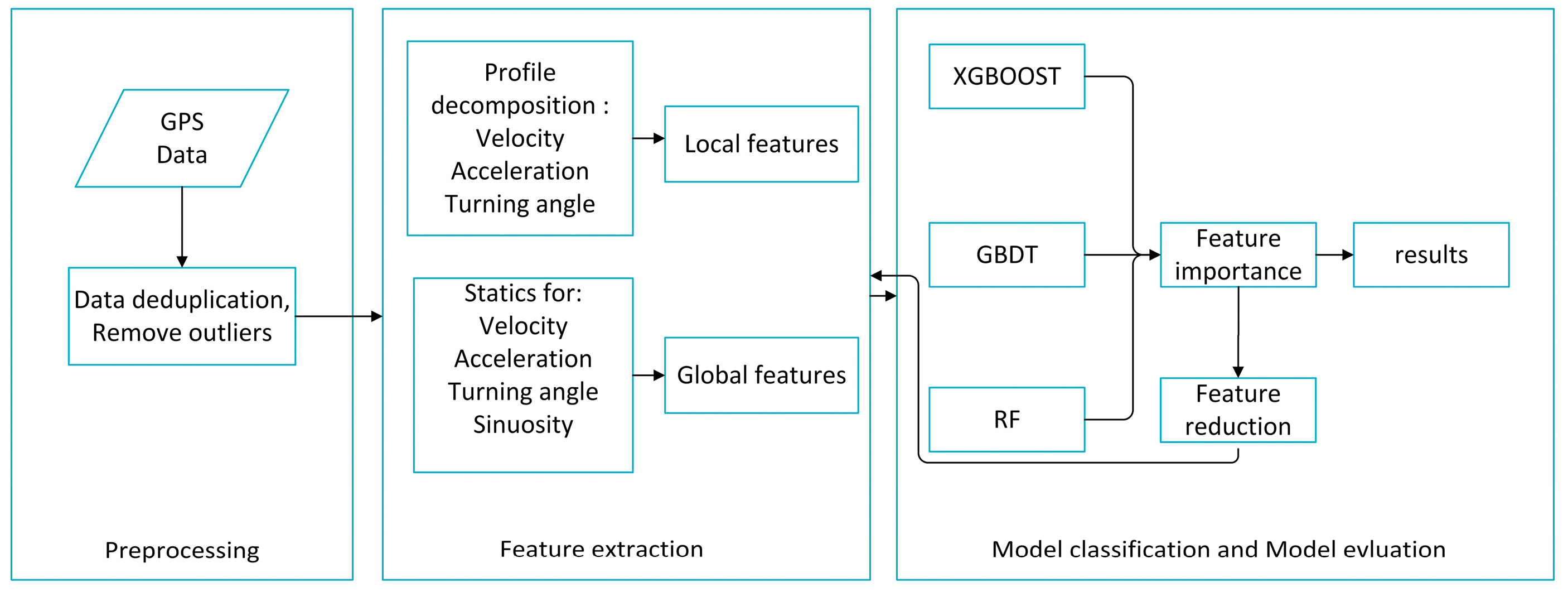
In this paper, we propose a method to identify six different transportation modes including walking, cycling, driving a car, taking a train and taking subway using GPS data. The main modules of our methodology for identifying transportation modes is shown in
Figure 1 and includes data preprocessing, feature extraction, model classification and model evaluation. Raw GPS data were first preprocessed into trajectories, and then global and local features were extracted before using the ensemble method to classify the different transportation modes. From the ensemble method, we obtained the important extracted features and removed the unimportant features, before results were finally obtained. Each step is detailed in the following sections.
3.1. Data Preprocessing
For a better performance, two data preprocessing techniques were employed in this study. First, we removed the duplicate data in the dataset as some GPS points were recorded more than once due to recording errors on the GPS device. Second, according to common sense, we removed some outlier trajectories, which were deemed abnormal. For instance, if the average speed of a trajectory marked as “walking” exceeded 10 m/s, or if the average speed of a trajectory marked as “biking” exceeded 25 m/s, we identified them as abnormal trajectories and removed them from the dataset.
3.2. Feature Extraction
Feature engineering plays an important role in recognizing the transportation modes. Feature engineering is the process of using domain knowledge to create features to enable machine learning methods to work well; to achieve differentiated results in the recognition of transportation modes and to extracted a large number of features from the processed GPS trajectories. These features can then be categorized into global features and local features. Global features refer to descriptive statistics for the entire trajectory, which makes trajectories more comparable, and the local features extracted by profile decomposition reveal more detail in movement behavior. The following subsections explain each category feature in detail.
3.2.1. Global Features
First, we calculated four movement parameters from the original trajectories: speed, acceleration, turn angle (the direction of the two consecutive points) and sinuosity (its winding path divided by the distance). Following that, we used the statistics method [
22] to extract global features based on the above-mentioned movement parameters and are listed as follows:
- (1)
Mean: This is a measure of the central tendency of the data sets.
- (2)
Stand deviation: This is a measure that is used to describe the dispersion of a set of data values.
- (3)
Mode: The mode represents the value that occurs most frequently in the sets; the parameters are first rounded into integers as the parameters are continuous values.
- (4)
Top three value, Minimum three value: These parameters are to reduce the error brought by the abnormal point with positional errors.
- (5)
Value ranges: The maximum value minus the minimum value.
- (6)
Percentile: A measure that represents the value below a given percentage of observations which is used in statistics. In this paper, we select the 25th percentile (lower quartiles) and 75th percentile (upper quartiles).
- (7)
Interquartile range: This parameter is equal to the difference between the lower and upper quartiles.
- (8)
Skewness: This is a measure of asymmetry of the probability distribution of a real-valued random variable about its mean, which can be used to describe the distribution of movement parameters, and is defined by:
where
represents the average of the data, and
represents the standard deviation of the data.
- (9)
Kurtosis: A measure of the “tailedness” of the probability distribution of a real-valued random variable and can also be used to describe the distribution of movement parameters compared to the normal distribution, and is defined by:
where
represents the average of the data, and
represents the standard deviation of the data.
- (10)
Coefficient of variation: This is a standardized measure of dispersion of probability distribution or frequency distribution, when the measurement scale difference is too large, it is inappropriate to use standard deviation to measure the parameters as the standard deviation is always understood in the context of the mean of the data but the
is independent of the unit. Therefore, it can handle the problem of different unit or large measurement scale, and is defined by:
where
represents the average of the data, and
represents the standard deviation of the data.
- (11)
Autocorrelation coefficient: This is the cross-correlation of a signal with itself at different points in time (what the cross stand for). First the coefficient of auto-covariance is calculated by:
where
represents the average of the data.
Then, we can calculate the autocorrelation coefficient, which is defined by:
It is a mathematical tool for finding repeating patterns, and represents the correlation between the values of the process at different times.
Secondly, in addition to these statistical features, we used other features proposed by Zheng et al. [
15], which proved robust to traffic conditions and are listed as follows:
- (1)
Heading change rate: This measure is a discrimination feature to distinguish different transportation modes as proposed by Zheng et al. [
15]. It can be considered as the frequency in which people change their direction to certain threshold within unit distance, which can be used to distinguish motorized and non-motorized transportation modes, and is defined by:
where
represents the set of GPS points at which user changes direction extending to a given threshold, and
stands for the number of elements in
.
- (2)
Stop rate: The stop rate represents for the number of points at which the velocity of the user under a certain threshold in unit distance mentioned by Zheng et al. [
15], is defined by:
where
represents the set of points at which a user’s velocity below a giving threshold.
- (3)
Velocity change rate: This feature mentioned by Zheng et al. [
15] is defined by:
where
represents the collection of points at which the user’s velocity changes above a giving threshold, and the velocity change is defined by:
- (4)
Trajectory length: The total distance of the trajectory.
3.2.2. Local Features
We adopted the profile decomposition algorithm mentioned by Dodge [
23] to generate several local features. As the movement parameters (velocity, acceleration, and turning angle) change over time when a person is moving in the space, this becomes a profile or a function. First, the movement parameter is expressed as a time series, where the amplitude and change frequency will provide proof to describe the movement behavior and physics of the person. Second, we used two measures to decompose the movement parameters, where a deviation from the central line represents the amplitude variations over time. Sinuosity reflects the frequency variations with time change. These points were then divided into four categories including “low sinuosity and low deviation”, “high sinuosity and low deviation”, “low sinuosity and high deviation” and “high sinuosity and high deviation”, which are labeled 0, 1, 2, and 3, respectively. More details can be found in Reference [
23].
Next, a series of features were extracted from the profile decomposition algorithm. This included the mean and standard statistics of segment length per decomposition class and per parameter; the count of changes of decomposition classes; and the proportion per decomposition class account for the total number of points.
A summary of the global features and local features is shown in
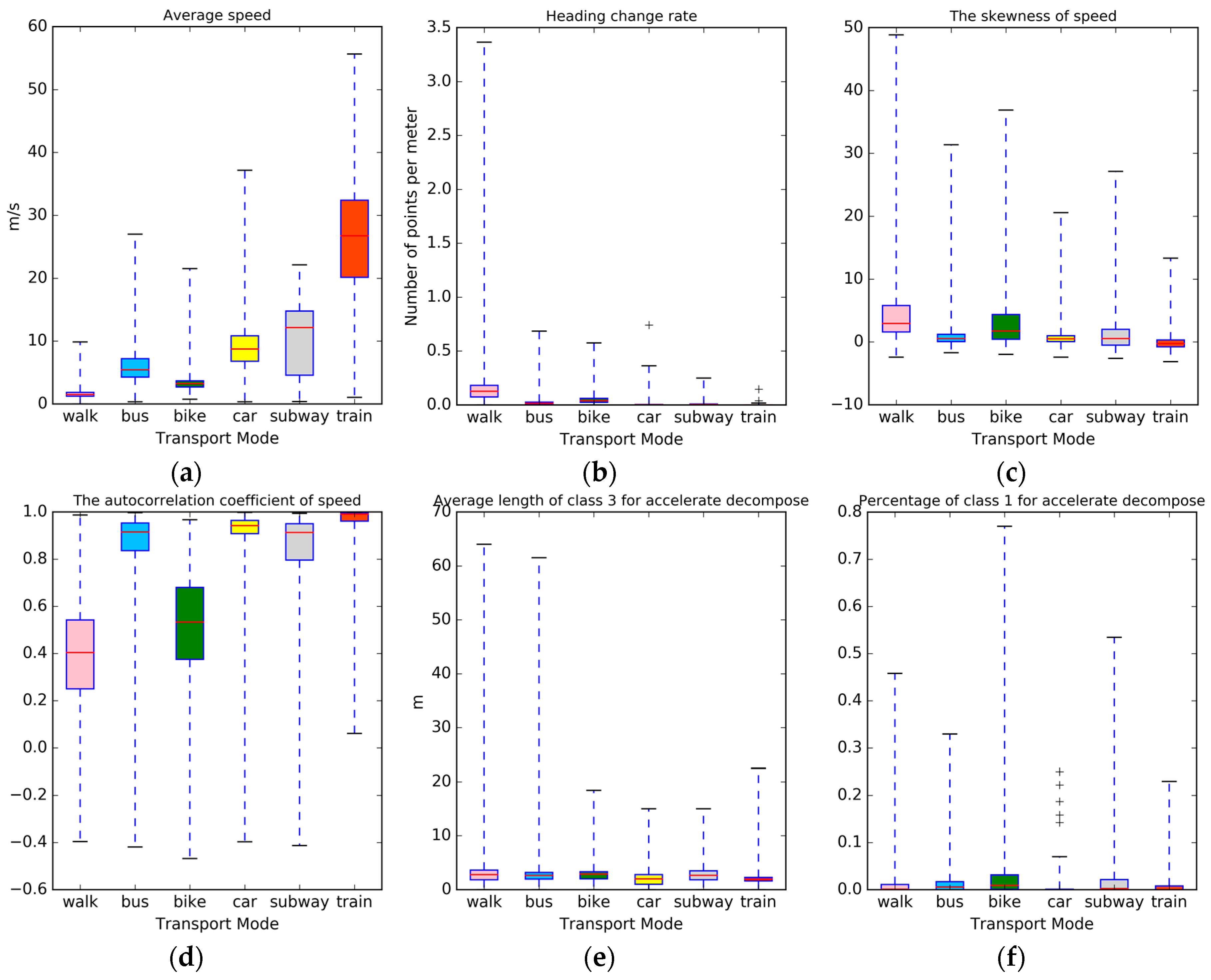
Table 2, where every trajectory extracts the global features and local features is mentioned. In
Figure 2, we plotted the distribution of six features mentioned above included four global features (a–d) and two local features (e and f); however, we found it difficult to differentiate between the different transportation modes using only a single feature. Nevertheless, these features can provide useful information in transportation identification when combined together. Therefore, 111 features were combined into the classification procedure, which is shown in
Table 2.
3.3. Model Classification and Model Evluation
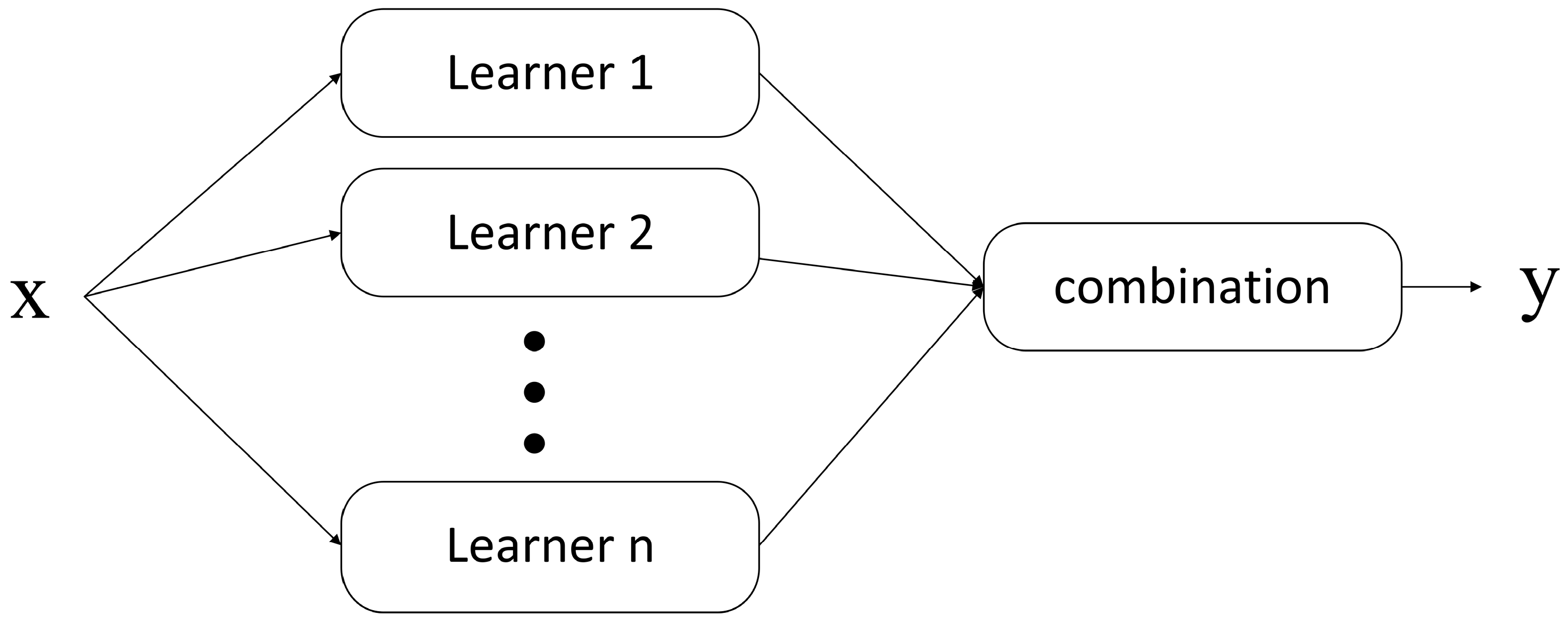
Ensemble methods train multiple base learners to solve the same problems, which differs from base learning algorithms. The basic structure of ensemble learning is shown in
Figure 3. Ensemble methods were highlighted by two pioneering works and have since become major machine learning algorithms. One empirical work, by Hansen and Salamon [
35], found that the combination of a set of classifiers often perform better than the best single classifier. The other pioneering work was theoretical, where Schapire [
36] proved that a combination set of weak learners was superior to a single stronger learner. Ensemble methods are widely used in many machine learning challenges; for example, Random Forest was used in 2010 Knowledge Discovery and Data Mining (KDD) Cup to win the first prize [
20], the Gradient Boosting Decision Tree (GBDT) was used in the Netflix prize [
18], and XGBoost was successfully used in Kaggle competition and 2015 KDD Cup [
19].
K-Nearest Neighbor [
13,
25], Decision Tree (DT) [
7,
13,
14,
15,
24,
25] and Support Vector Machine (SVM) [
12,
13,
14,
17,
23,
25] have been widely used to classify transportation modes and have resulted in good performance. However, in this paper, we choose to use the tree ensemble models to classify transportation modes instead of using the above-mentioned methods. The reasons why we selected the tree ensemble methods are as follows. Firstly, tree ensemble methods perform better than traditional methods (KNN, DT, SVM) not only in higher prediction accuracy, but also in superior efficiency, which has been proved in many machine learning challenges. Secondly, the parameter tuning in tree ensemble methods was easy to conduct. Thirdly, deep learning or neural network was not used as the data volume is insufficient and the parameter tuning in deep learning was too complex. The ensemble methods used in this paper were Random Forest (RF) [
37], Gradient Boosting Decision Tree (GBDT) [
34] and XGBoost [
19].
In the next section, we introduce the basic principles of these three models briefly where more detail can be found in the corresponding references, and then the evaluations of our method are explained.
3.3.1. Random Forest
Random Forest was proposed in 2001 [
37] and used the bagging method to ensemble many decision trees with the final classification result obtained based on the majority votes. Random Forest was widely applied at each classification task, and achieved great performance. The main steps are as follow:
- (1)
The column sampling technique was used to select the train set for growing the tree. Not all samples fit into the tree growing, but the boostrap method was used to generate the training set.
- (2)
The row sampling technique was used to select m (m << M) variables from M input variables, where the best spilt was found on these variables, to help contribute in overcome overfitting.
- (3)
Each tree in the forest grew completely without any pruning.
3.3.2. Gradient Boosting Decision Tree
The GBDT is a widely used method for classification and regression problems proposed by Friedman [
34], which produces a learning model in the form of a combination of a set of weak prediction models, typically decision trees. The difference between GBDT and the traditional Boost is that every iteration in GBDT is to reduce the residual of the last iteration. In order to eliminate the residual error, the GBDT method establishes a new model on the direction of gradient. The GBDT is also a similar method to RF in that it combines a set of weak learners. The main difference between the GBDT and RF is that the tree in the GBDT is fit on the residual of the former tree, so that the GBDT model can try to reduce the bias, whereas RF tries to reduce the variance. Thus, RF can be trained in parallel, but the GBDT cannot, therefore, the GBDT was superior to RF in many challenges [
18,
19].
3.3.3. XGBoost
XGBoost [
19] is an optimized distributed gradient boosting library designed to be highly efficient, flexible and portable. XGBoost provides a parallel tree boosting that solves many data sciences in a fast and accurate way. The advantages of this method over the traditional GBDT are as follows:
- (1)
Additional regularization terms can be added to help smooth the final learnt weights to avoid over-fitting.
- (2)
Second-order approximation of the loss function can be used to quickly optimize the objective in the general settings.
- (3)
Shrinkage (introduced by Friedman [
34]), can be used to reduce the influence of each individual tree and leave more space for future trees.
- (4)
The column technique in RF can be used for reference, in order to prevent over-fitting and to speed up computations of parallel algorithms.
- (5)
Some techniques, including blocks for out-of-core computation and cache-aware access can be used to make tree learning faster.
3.3.4. K-Fold Cross-Validation
The K-Fold Cross-Validation is a technique to derive a more accurate f model and to help tune parameters. The original samples are randomly partitioned into k equal parts; of the k parts, a single part is used as the validation dataset, and the remaining k-1 subparts are used as the training dataset to construct the model. The same procedure is repeated k times, with a different validation dataset is chosen each time, before the final accuracy of the model is equal to the average accuracy obtained each time. The advantage of this technique over repeated random sub-sampling is that all samples are used for both training and validation, and each sample is used for validation exactly once.
3.3.5. Evaluations
In order to evaluate the performance of different classification models, several methods were used in this study, including precision, recall, F-score, confusion matrix, Receiver Operating Characteristic curve and Area Under The Curve. For classification problems, samples were divided into four categories: true positives; true negatives; false positives; and false negatives (
Table 3).
Precision is the fraction of retrieved documents that are relevant to the query, and recall is the fraction of the documents that are relevant to the query that are successfully retrieved. Precision and recall are thus defined as:
In order to measure the overall performance of the model, the F-score was considered, which contains both the precision and the recall.
The confusion matrix is a specific table layout that allows the visualization of the performance of an algorithm, which shows the error rates, precision and recall values. The ROC curve illustrates the performance of a classifier system as its discrimination threshold is varied, and is created by plotting the true positive rate (TPR) against the false positive rate (FPR) at various threshold settings, thus providing tools to select possible optimal models. We can use the areas under the curve to measure the performance when the two ROC-curves were cross, which is called the AUC.
4. Results and Discussion
A dataset collected by the Geolife project [
12,
13] by 182 users over a period of five years (from April 2007 to August 2012) was used to validate the performance of the ensemble model. This dataset is widely distributed in over 30 cities of China, as well as cities located in the USA and Europe and contains 17,621 trajectories with a total distance of 51 km and a total duration of 50,176 h. Up to 91.5% of the trajectories are logged in a dense representation, e.g., every 1–5 s or every 5–10 m per point. In the dataset, 73 users labeled their trajectories with their starting transportation mode or when their mode changed.
Figure 4 presents one example of the trajectories in the Geolife dataset, and these labeled trajectories were used to conduct the experiment.
After data preprocessing, 7985 trajectories were extracted. The dataset was separated into a training set (consisting of 70% of the data) and a testing set (30% of the data). The distribution of the number of different categories is shown in
Table 4. As the distribution of the different categories was unbalanced, it was unreasonable to base our evaluation on accuracy alone, despite this being commonly done in the previous literature. Furthermore, it was difficult to evaluate the performance of the model based on a single measure as these measures are sometimes the same. Thus, in our study, different evaluation techniques were used, including Precision, Recall, F-Score, ROC cure and Confusion matrix. We used overall misclassification rate which is obtained from five-fold Cross-Validation to tune the parameters. The detailed experiments are shown below:
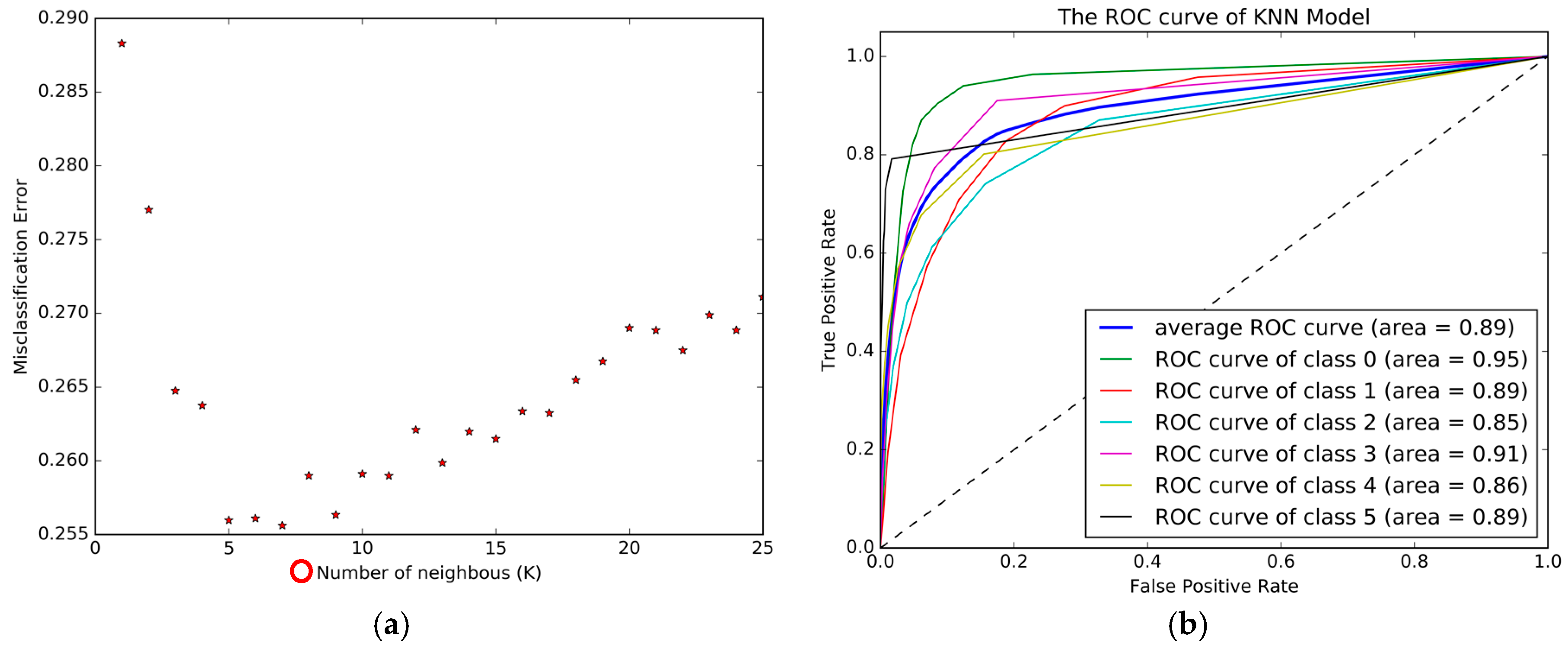
4.1. K Nearest Neighbor
The KNN model was implemented in the Python software along with “sklearn” package. The tuning parameter in the KNN model was the number of neighbors.
Figure 5a shows the change of misclassification error with the number of neighbors, which was obtained using five-fold Cross-Validation. From
Figure 5, we can see that the highest accuracy was achieved when K was 7, and the overall accuracy was 74.44%. The ROC curve is plotted in
Figure 5b, and the Confusion matrix is presented in
Table 5.
Figure 5b and
Table 5 show the poor performance of bus, bike, car, subway and train, which led to the conclusion that the KNN model found it difficult to differentiate the different transportation modes.
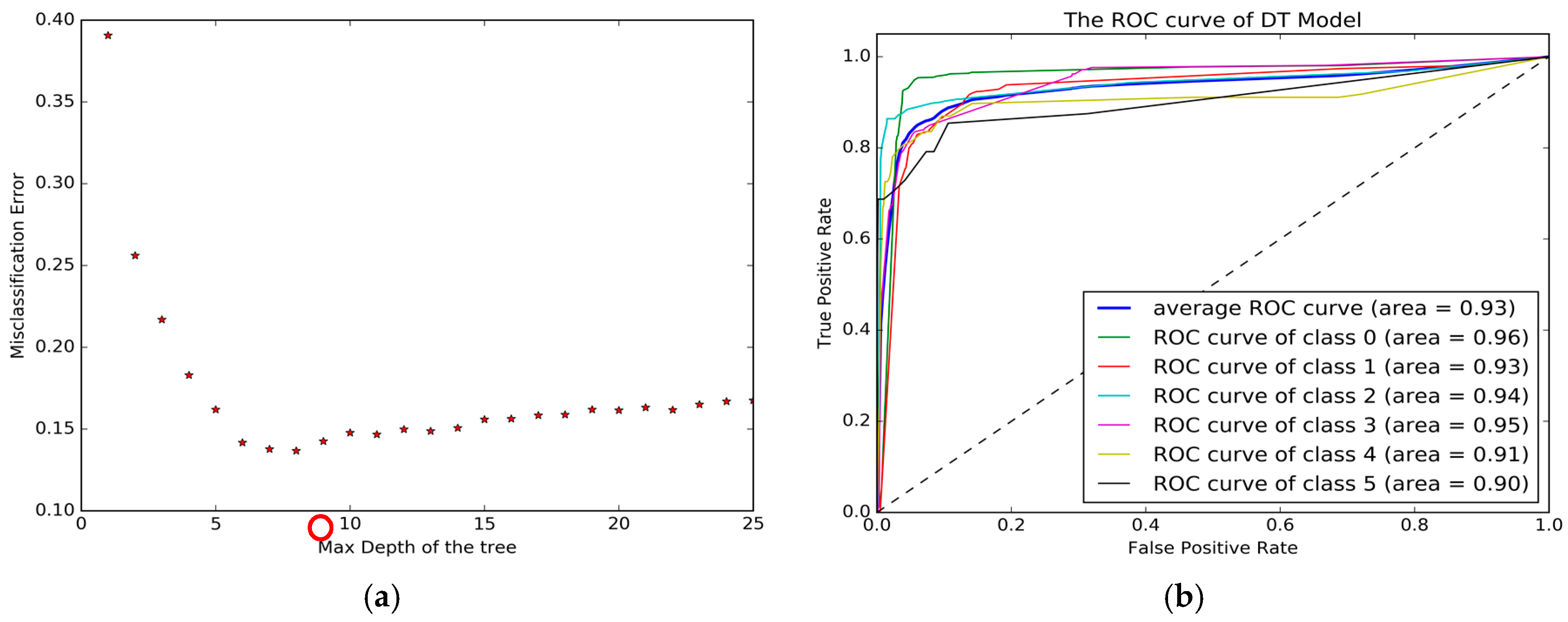
4.2. Decision Tree
The decision tree model was implemented in the Python software along with “sklearn” package. The tuning parameter was the maximum depth of the tree and was used to control over-fitting.
Figure 6a shows how the depth of the tree impacts the performance of the model. The best performance was 86.05%, and was achieved when maximum depth was 7. The Confusion matrix is presented in
Table 6, and the ROC curve is plotted in
Figure 6b. In
Figure 6b and
Table 6, we can see that the performance of the DT model was better than the KNN base in most of the evaluation measures; however, it is still unable to effectively identify transportation modes including car, subway and train.
4.3. Support Vector Machine
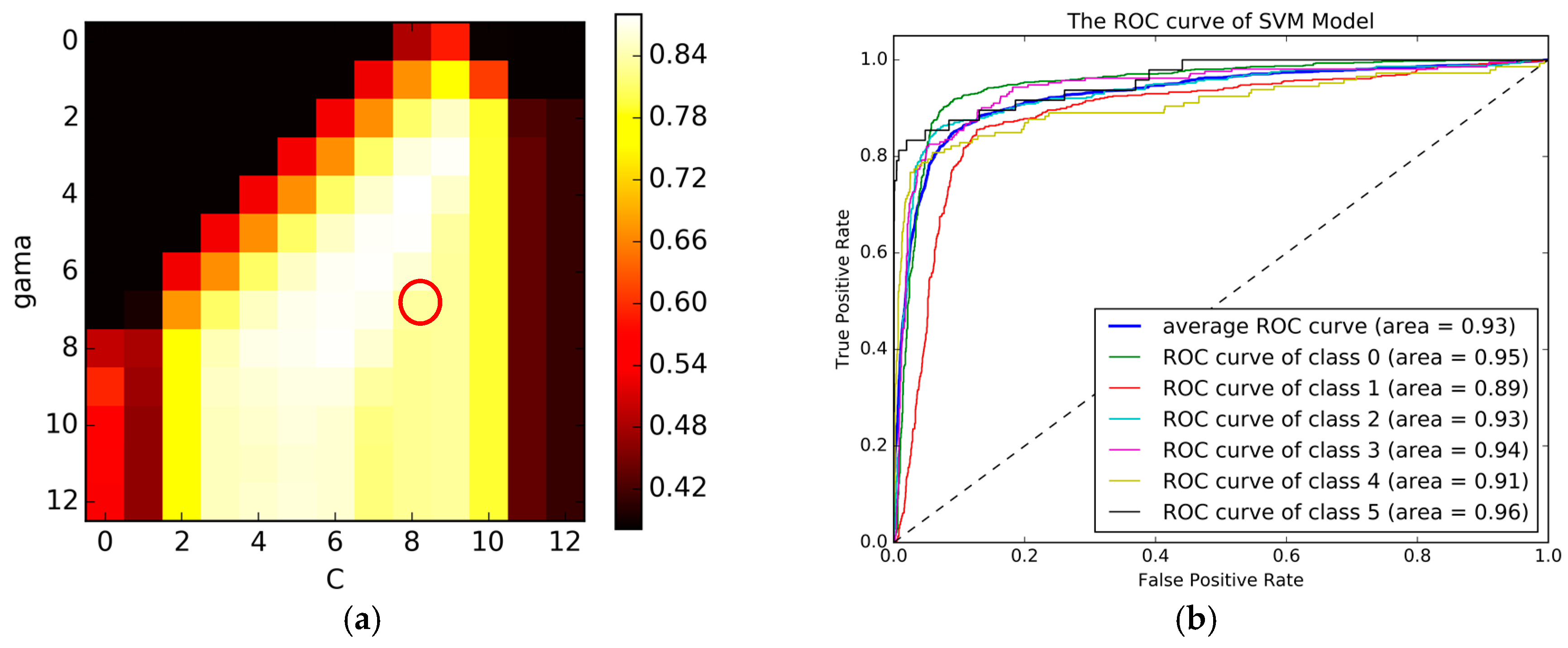
The SVM model was implemented in the Python software along with “sklearn” package. The tuning parameters contained regularization parameter (c) and Gaussian parameter (σ).
Figure 7a provides a heat plot that demonstrates how the regularization parameter (c) and the Gaussian parameter (σ) impacted the performance of the SVM model. The optimal parameters (c, σ) of the model were eight and five, respectively, and are circled in red. The highest accuracy was 87.69%, the Confusion matrix for the best SVM model is presented in
Table 7 and the ROC curve is plotted in
Figure 7b. In
Figure 7b and
Table 7, we can see that although the SVM model performed better than both the KNN and DT models, it still cannot effectively identify transportation modes including car, subway and train.
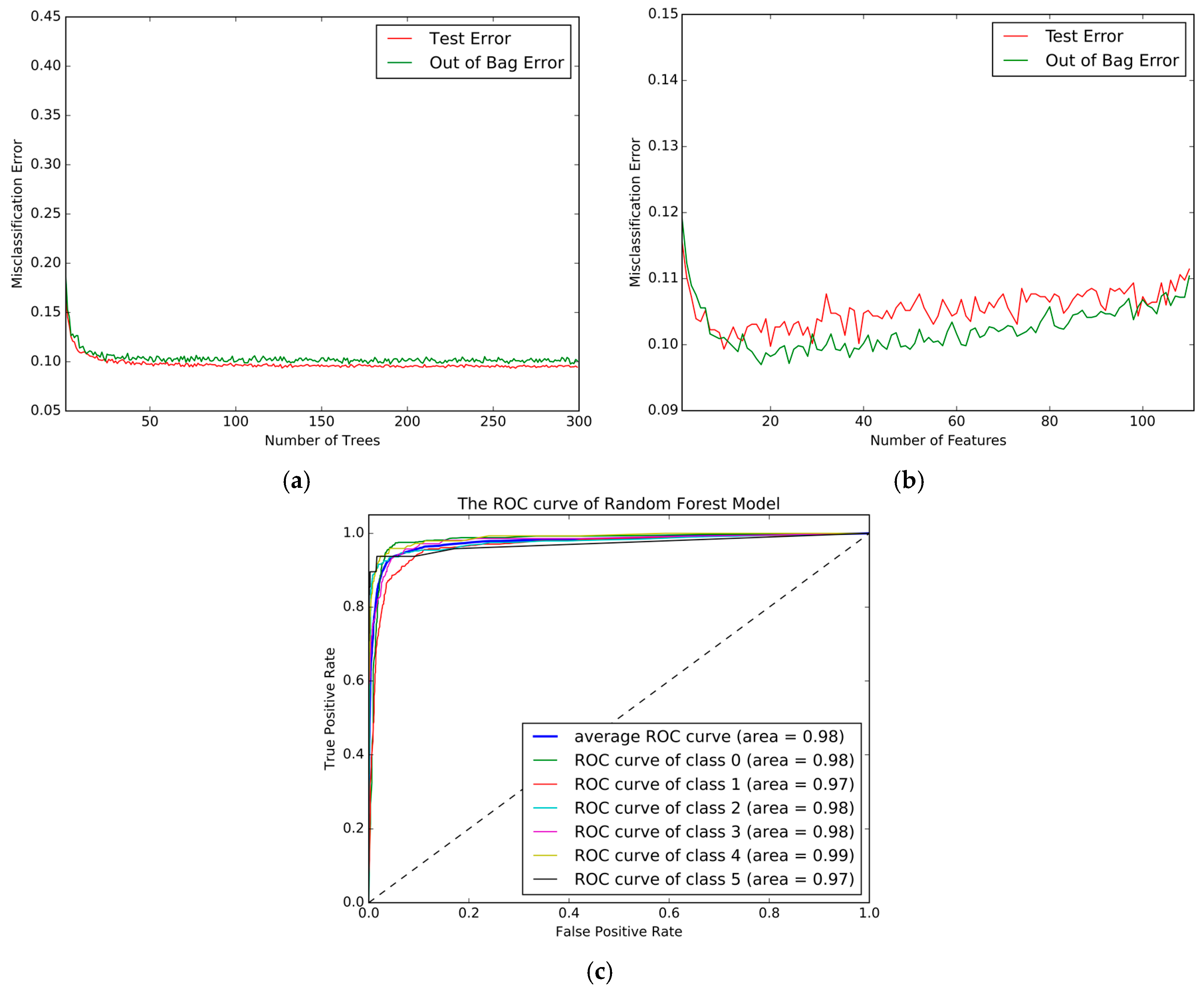
4.4. Random Forest
The Random Forest model was implemented in the Python software along with “sklearn” package.
Figure 8a shows the change of Test-Error and the Out of Bag Error with number of the tree, and
Figure 8b shows the influence of the number of features. From these two figures, 200 trees and 16 features generated the best performance.
Table 8 shows the Confusion matrix for the best RF model, and the ROC curve is plotted in
Figure 8c. The best five-fold Cross-Validation accuracy was 90.28%, and shows that it has remarkably outperformed the KNN, DT and SVM models. Furthermore, compared to the other models listed above, we found that the RF model could effectively identify the transportation modes that other models could not, such as car, subway and train. The detection accuracy of these models showed a significant improvement over the above models.
4.5. Gradient Boosting Decision Tree
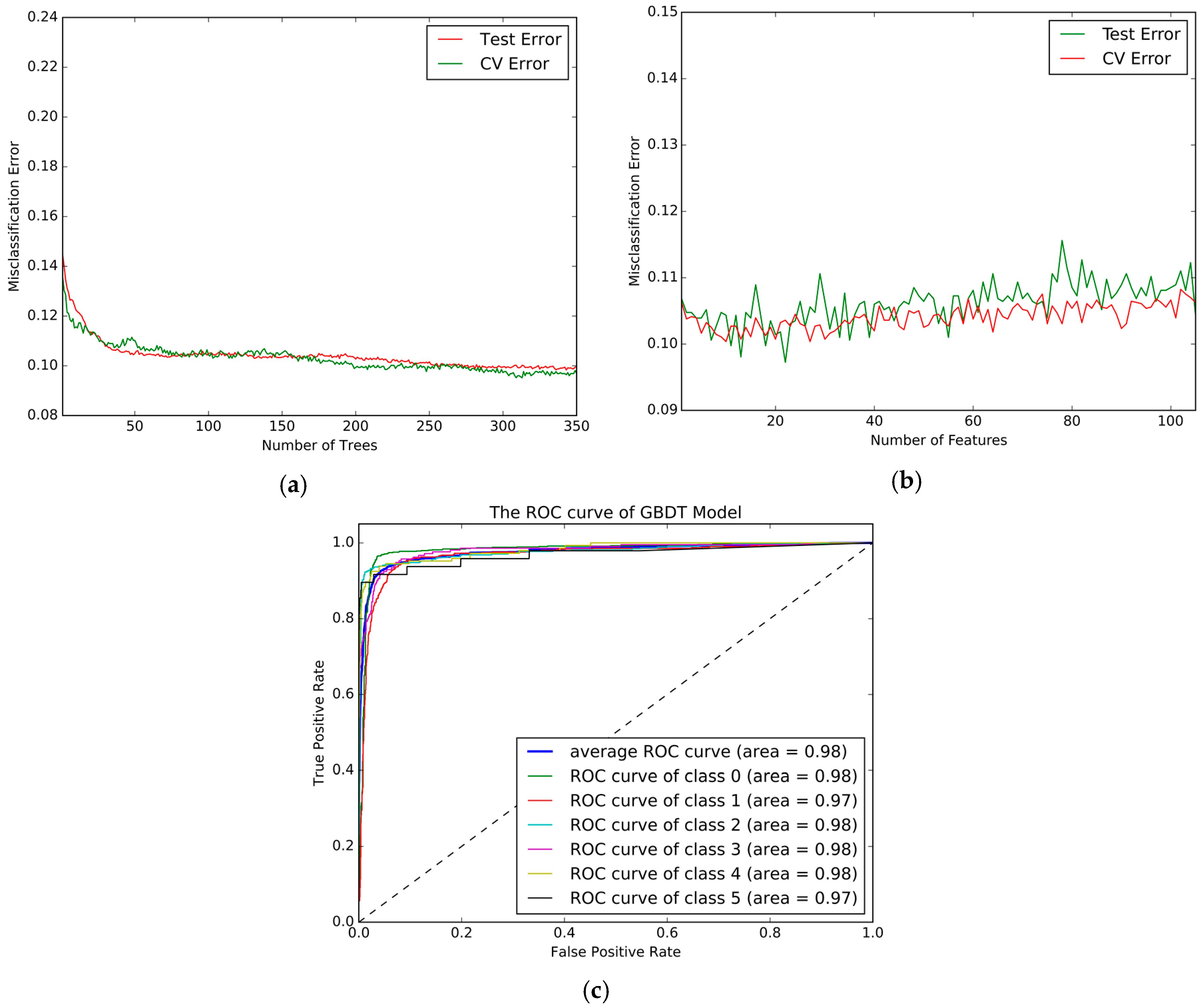
The GBDT method was implemented in the Python software along with “sklearn” package. The tuning parameters in the GBDT method contained the number of trees, the number of features, and max depth.
Figure 9a shows the change of Test-Error and CV (five-fold Cross-Validation) Error with number of the tree,
Figure 9b shows the influence of number of features used in each tree. The highest accuracy (90.46%) was achieved when 500 trees, 16 features, and a max depth of six were used. The Confusion matrix for the best GBDT models is shown in
Table 9 and the ROC curve are plotted in
Figure 9c. The results imply a small improvement over the RF model, but GBDT is more time-consuming than RF model as it cannot process in parallel (which can be seen in the part model comparison).
4.6. XGBoost
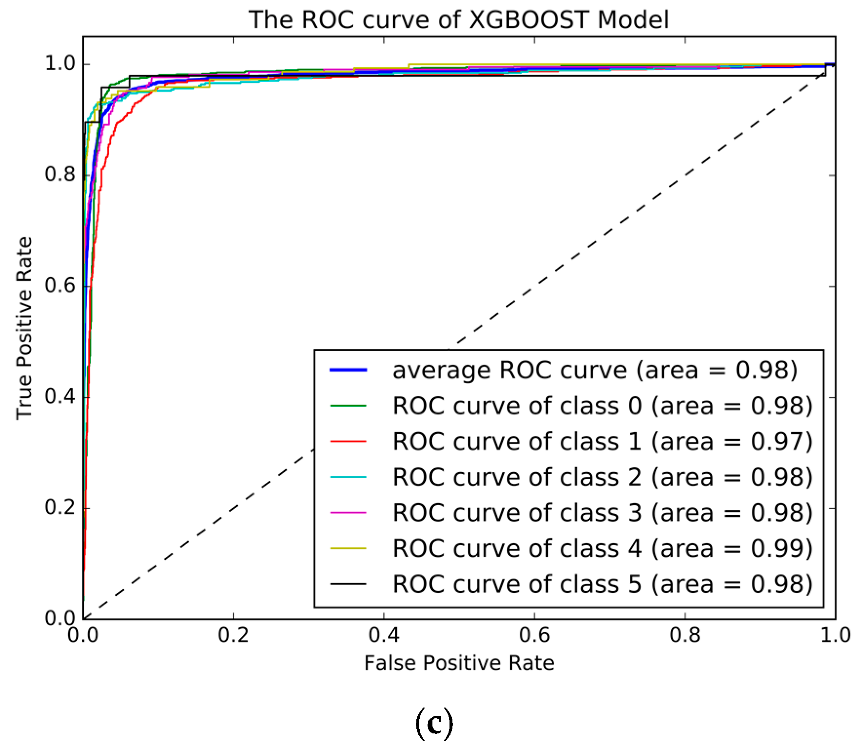
The XGBoost method was implemented in the Python software along with “XGBoost” package. The tuning parameters in XGBoost included “num_round”, “eta”, “max_depth”, “scale_pos_weight” and “min_child_weight”. We used the five-fold Cross-Validation to tune the parameters which included the following steps: First, we selected a relatively high learning rate and determined the optimum number of trees for this learning rate. Second, we tuned tree-specific parameters (max_depth, min_child_weight and scale_pose_wight) for the decided learning rate and the number of trees. Third, we tuned the regularization parameters (lambda, alpha) for XGBoost, which can help reduce model complexity and enhance performance. Fourth, we lowered the learning rate and decided on the optimal parameters. We have provided two example of the parameters tuning process, other process can be found in Reference [
38].
Figure 10a shows the influence of the number of iterations on the misclassification error and
Figure 10b shows the influence of the number of features used in each iteration. Using this method, the highest accuracy was 90.77% with the parameters set as follows: num_round = 500, eta = 0.05, max_depth = 6, scale_pose_weight = 5, and min_child_weight = 1. The Confusion matrix for the best XGBoost models is shown in
Table 10 and the ROC curve is plotted in
Figure 10c, and shows an improvement greater than that of the GBDT model, and more discriminating in many transportation modes, with the train speed was faster than the GBDT model which will be proved in the next section.
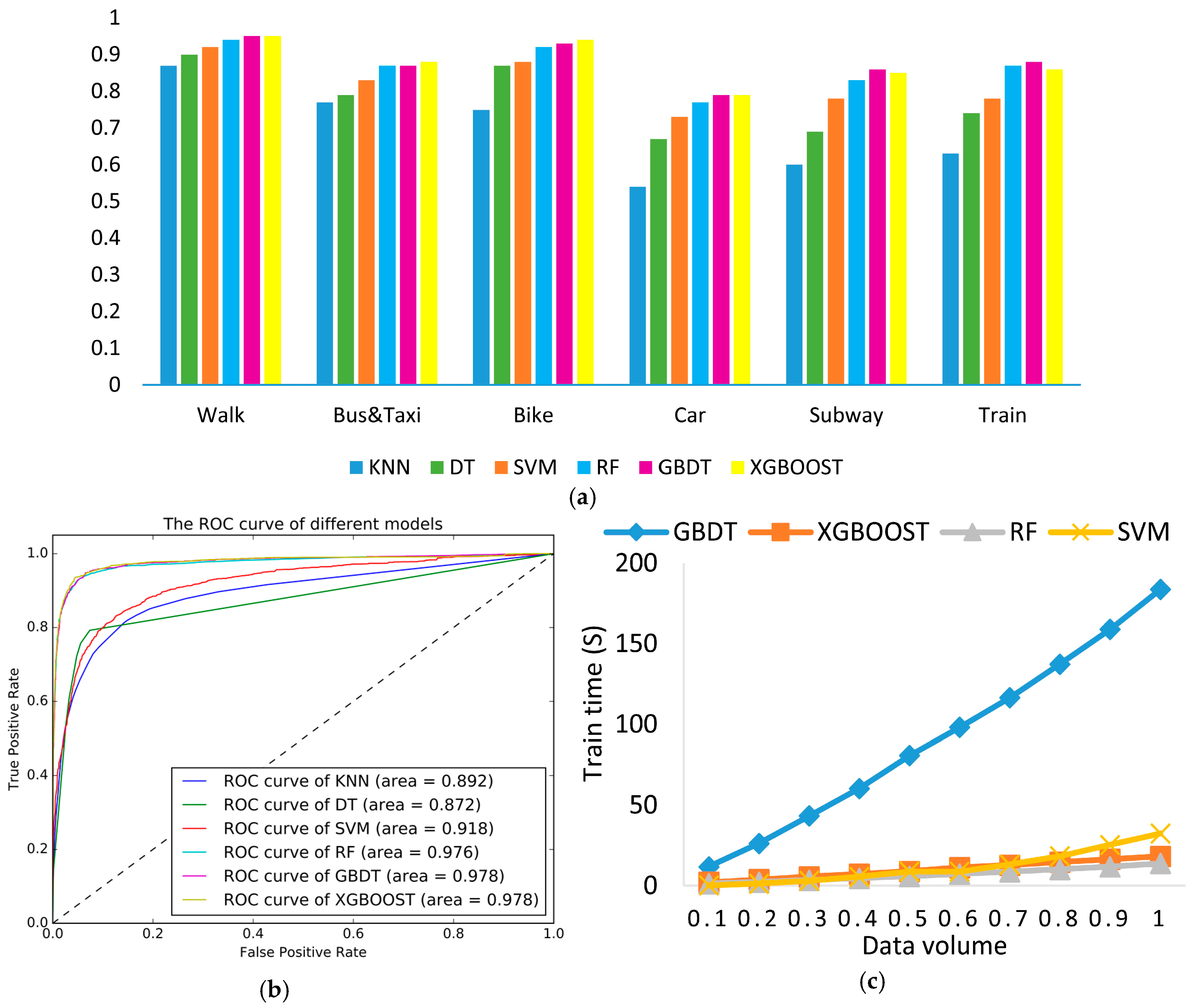
4.7. Model Comparison
Based on the above results, the F-score measure was calculated and can be seen in
Figure 11a. It is obvious that the tree-based ensemble models achieved a higher F-score than the DT, SVM and KNN models.
Figure 11b shows the ROC curve and the AUC measure of different classification models. In
Figure 11b, it can be clearly seen that tree-based ensemble models achieved superior results to the DT, SVM and KNN models based on ROC and AUC measures. Meanwhile,
Figure 11c shows the computation time of the different models where the XGBoost and RF model consume less time than others, and can handle large volumes of data in the future. Considering the different evaluation measures, we finally concluded that the tree ensemble methods performed better than the traditional machine learning methods (K-Nearest Neighbor, Support Vector Machines and Decision Tree), and out of the tree ensemble methods, the XGBoost model produced the best performance, with the highest accuracy 90.77%, which was a nearly 3% improvement compared to the SVM model.
These results also suggest that the classification errors mainly occurred between the car and bus classifiers, as these two transportation modes always perform similarly in the GPS trajectory. One solution to reduce the error is to add more accurate sensors to improve the classification performance in feature work, such as gyroscopes and rotation vectors. Another solution is the use of GIS information to create more distinguished features; however, these two methods have several limitations, which are mentioned earlier. Therefore, the use of these two solutions depends on the detailed application. Furthermore, tree-based ensemble methods can still efficiently identify different transportation modes by combining these features into the classification procedure.
4.8. Feature Importance and Feature Reduction
As mentioned earlier, 111 features were extracted from the original GPS trajectory. To evaluate the validity of our feature extraction method, we compared our features with the following baseline features: (1) Global features: 72 dimensional features mentioned above; (2) Local features: 39 dimensional features mentioned above; (3) Zheng’s features: 12 dimensional features mentioned by Zheng [
15]; (4) Dodge’s features: 48 dimensional features mentioned by Dodge [
23]; and (5) Global + Local: the combination of global features and local features. We performed the experiments with the same dataset that used the same method but with different features.
Table 11 shows the misclassification error with different features in the same model. We still found that tree-based ensemble methods perform better than other methods in different features, and we concluded that our feature extraction method worked better in recognizing different transportation modes than other feature extraction methods. The combination of Global features and Local Features scores the lowest error rates.
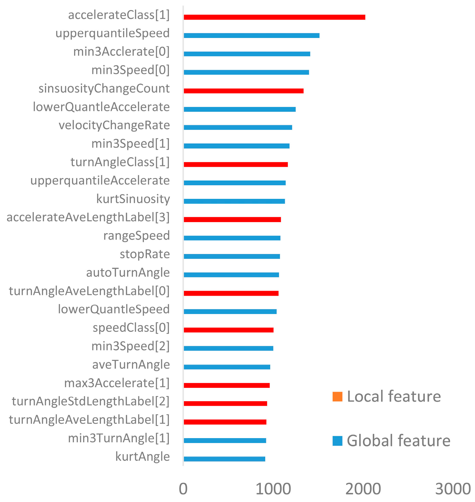
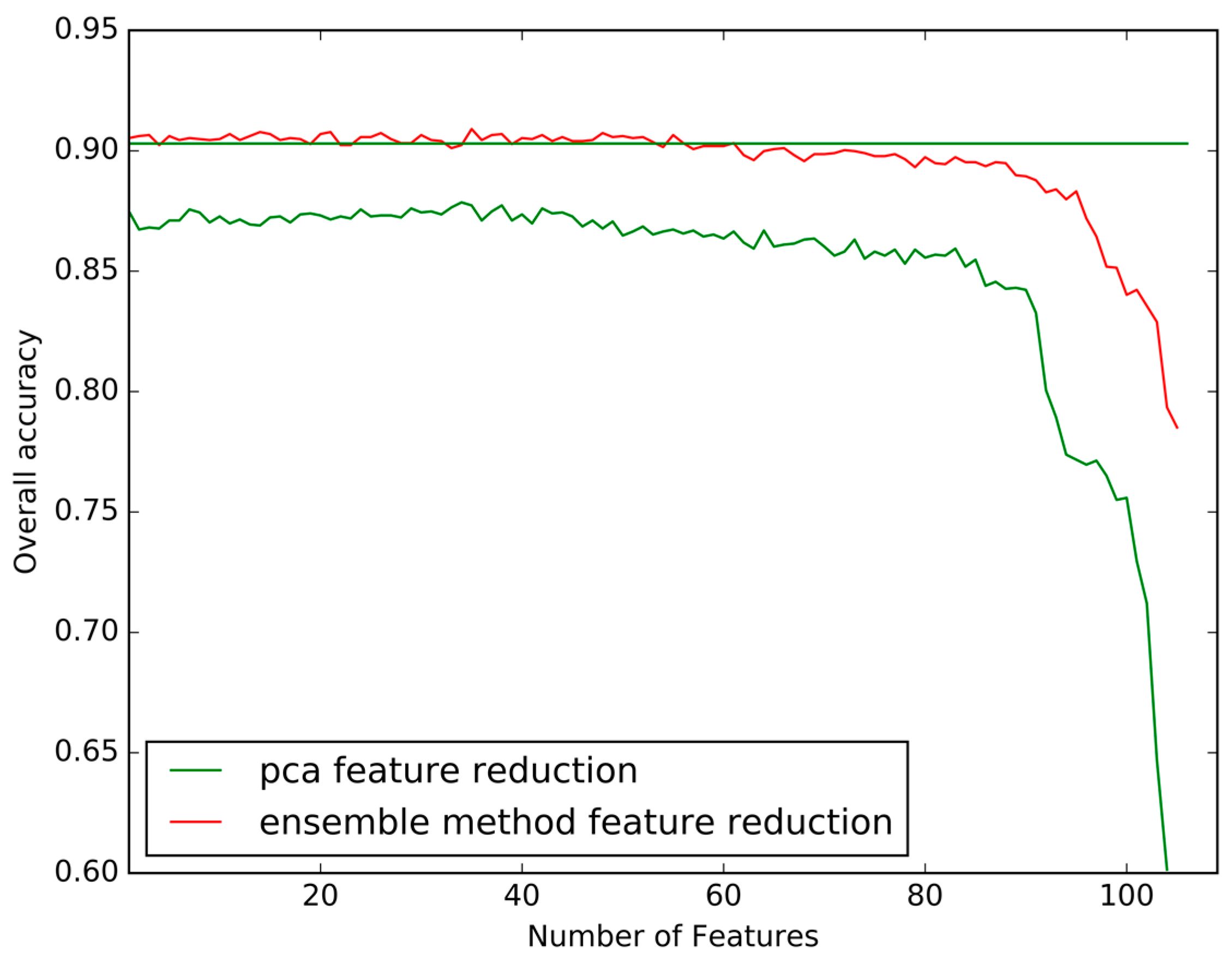
In most of the previous literature, the principal component analysis (PCA) is predominantly used to conduct feature selection prior to the classification stage. In our study, we used the tree-based ensemble method to carry out feature selection to reduce the model complexity after the classification stage, which is different from the feature selection method used in most of the literature. We removed the unimportant features one by one, and then recalculated the overall accuracy, where the importance of features was accessed based on the measure “weight”, which represents the number of times a feature is used to split the data across all trees. Therefore, the important features are features that are used frequently to split the data during the process of model construction. It was also able to discriminate between different transportation modes. In
Figure 12, the red line shows how the number of features removed by the ensemble methods impacted on overall accuracy, while the green line shows how the number of features reduced by the PCA method, In
Figure 12, it can be obviously seen that feature reduction method based on ensemble methods performed better the PCA method. Ensemble methods can still achieve highly predictive ability even when nearly 60 unimportant features are eliminated. Thus, 51 features can meet the algorithm to identifying the transportation modes.
Figure 13 shows the 25 most important features with different classification tasks. Items in red represent local features and blue items represent global features. We found that important features contained both global and local features, which proves that both kinds of features play an important role in transportation mode recognition task. In
Figure 13, we also found that important features contained a percentage of acceleration decomposition class which was labeled “high sinuosity and low deviation”, and follows upper quartiles of the speed and minimum value of acceleration.
5. Conclusions
An approach based on ensemble learning was developed to infer hybrid transportation modes that included walking, cycling, driving a car and taking a subway using only GPS data. To obtain a better performance, we first combined the global features generated by Statistics method and the local features extracted by trajectory segmentation. Second, we used tree-based ensemble models to classify the different transportation modes. These experiments revealed that a combination of global and local features made sense when detecting modes of transport. The experiments also proved that tree-based ensemble models performed better than the traditional methods (KNN, DT and SVM), using different evaluation techniques such as the F-Score, ROC curve, AUC and Confusion Matrix. Finally, the XGBoost model was found to the best out of the evaluation methods, with the highest accuracy from five-fold Cross-Validation of 90.77%. Furthermore, we used tree-based ensemble methods to conduct feature selection, which performed better than the PCA method.
In this paper, overall misclassification rate, which is obtained from five-fold Cross-Validation, is used for parameters tuning, and other measures are available as well, but due to the limitation of space, they are not introduced in detail. In order to process the imbalanced data, several methods can be applied in the future such as sampling methods (oversampling and undersampling) and weighted-learning. Future work will investigate how to explain the ensemble model more intuitively, as the ensemble method is like a black box and is not easy to intuitively explain. Another investigation needs to pay attention to how to integrate the data collected from different sensors or how to use GIS acquired information if necessary. Furthermore, approaches on how to segment the trajectory with only one transportation mode before the classify stage, as trajectories may contain several transportation modes at the same time, should be developed. Some deep learning algorithms could support feasible solution in terms of identifying transportation modes.


