According to the index feature of the three properties of the traffic flow data, the optimal referenced standard is extracted from the data set of the analysis domain. Then, the optimal referenced standard and referenced array set are used to calculate the grey relational degree in combination with the dataset of the analysis domain. Subsequently, the grey relational matrix can be obtained, and the cluster members can be calculated. Next, we use rough set theory, where cluster members are applied, and build the decision information table to complete the fusion for the weighting of the cluster members, according to which we need to calculate the rank of each data object using probability theory. We regard the first category as the highest priority, which means that the data object is closer to the referenced standard and simultaneously that the object is better, corresponding to the lightest traffic congestion degree.
4.1. Grey Relational Clustering Steps
4.1.1. Extracting Optimal Referenced Standard according to the Characteristics of Traffic Flow Data
Because the problem of clustering analysis is solved based on a given indicator system, it is very important to choose the appropriate indicator to achieve reasonable and appropriate clustering. There are three properties for each from a data source, and based on the indicator attribute of the data object, the optimal reference standard can be extracted from the data source. Specific instructions are as follows.
We know that the three properties units are different; therefore, we first need to convert the data to the same format. “↑” indicates that the property value is greater and thus better; “↓” indicates the opposition. (a, b), where a and b are numbers, indicates that, if the property value of a data object is in this interval, the value will be better.
Extract the optimal referenced standard according to the characteristics of the three properties, and its expression is , which is described as follows:
Considering the characteristic of the traffic flow velocity as “↑”, we use
Considering the characteristic of the traffic flow density as “↓”, we use
Considering the characteristic of the traffic flow volume as “↓”, we use
4.1.2. Data Normalization Processing
Because there are different types of data, the units are also different. According to the characteristics of the properties, the data of the analysis domain are processed using different measures, and the data are compressed to (0, 1). The processing is as follows:
For the traffic flow velocity of the whole data set, we use
For the traffic flow density of the whole data, we use
For the traffic volume of the whole data set, we use
is the original matrix element in the above Equations (5)-(7) and is normalized to
, where
represents the maximum of the
jth column and
represents the minimum of the
jth column, and anything inside of braces is the limiting condition. After normalization, we obtain (
p + 1) matrices, namely,
where
can be acquired by normalizing the optimal referenced standard
and the comparative object set. Meanwhile,
can be acquired by normalizing the referenced array set and the comparative object set, where
and
are defined as
The last row of the matrix is normalized to the optimal referenced standard sequence, and the last row of the matrix is the pth normalized referenced standard array.
4.1.3. Calculating Grey Relational Degree and Generating Grey Relational Similar Matrix
(1) The grey relational degree reflects the high degree between two comparative objects. For example, we focus on calculating the grey relational degree of the matrix
. The formulas are as follows (Equations (9) and (10)):
where
is the resolution coefficient, which has a range of 0 to 1. Generally, we assume that
is 0.5.
is the correlation coefficient between
and
at the
kth point. The grey relational degree is expressed by
, where
is regarded as the referenced sequence and
is regarded as the comparative sequence. Similarly, we can obtain
when
is regarded as the referenced sequence and
is regarded as the comparative sequence. Then,
are regarded as the referenced sequence; meanwhile, the (
n + 1) sequences are regarded as comparative sequences (the (
n + 1) sequences are not only referenced sequences but also comparative sequences). Finally, we calculate the grey relational degree matrix
according to the grey relational analysis, where
is obtained based on
A0 and consists of any
. Similarly, we can calculate the grey relational degree matrices
based on
.
(2) Calculate grey relational similar matrix G
We calculate the similarity elements in G. G0, for example, is the grey relational similar matrix obtained when is regarded as the referenced sequence, and the (n + 1)th row grey relational similarity elements of G0 are calculated when is regarded as the optimal referenced sequence. Similarly, we can obtain p + 1 grey relational similar matrices: .
4.1.4. Grey Relational Degree Clustering Analysis
Based on
G,
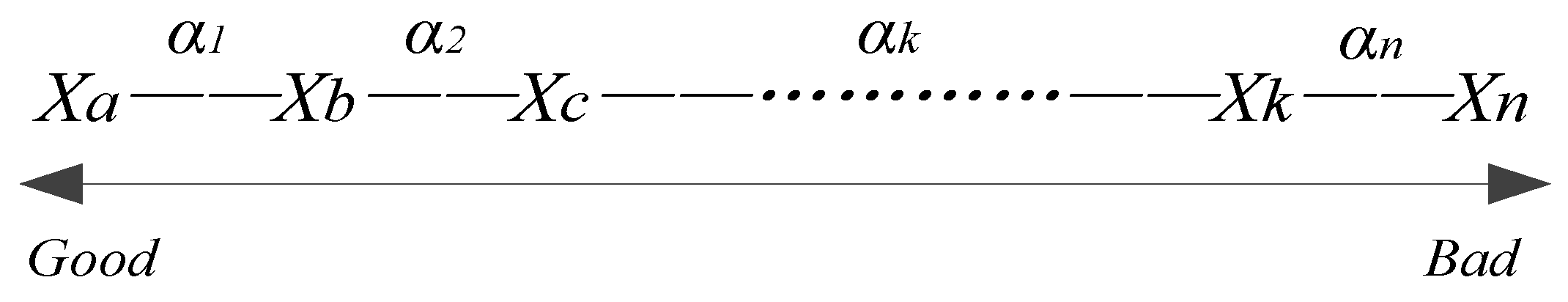
i.e., the grey relational similar matrix, we construct the maximal relational tree, which consists of the values of the last row elements ordered in
G. This is shown in
Figure 3.
Based on
G0, we can obtain
, which is also called the closeness degree between
and
. The greater
is, the closer
and
are; in contrast,
and
are further away for decreased
. Based on
Figure 3, the maximal relational tree with closeness degrees is generated, as shown in
Figure 4, where
represents the closeness degree between
and
.
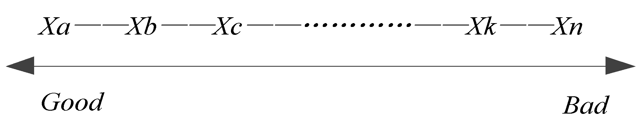
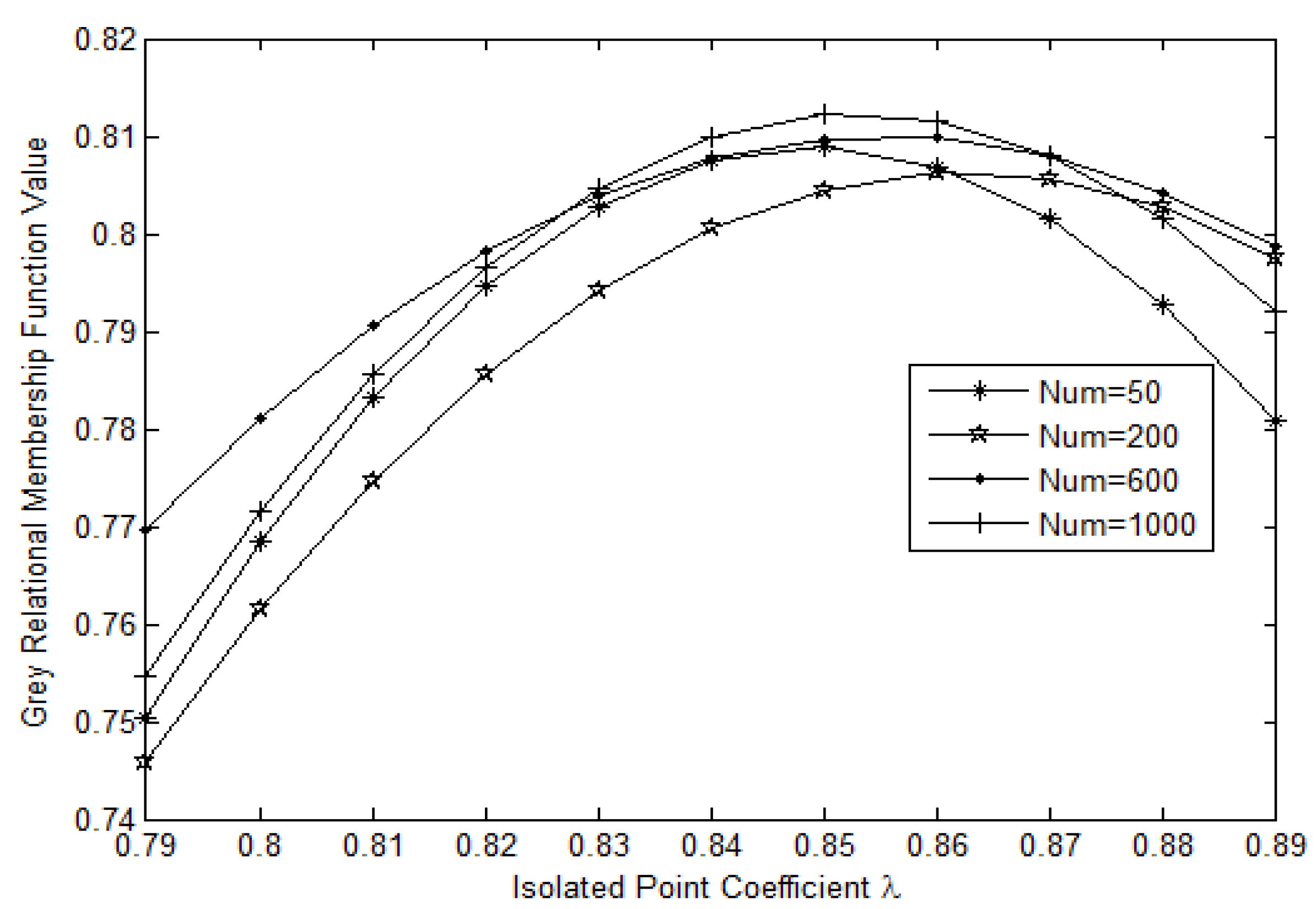
Based on
Figure 4, we set the isolated point coefficient
, which is in the interval (0, 1). We cut the tree when the closeness degree is less than
and when adjacent branches exhibit substantial differences. Therefore, the disconnected tree is used to make its connected branches form
k levels of clusters along the horizontal. We consider the closest branch as the first level and the loosest branch as the
kth level (If
k ≥ 4, we also classify the fifth branch, the sixth branch, the seventh branch, and even the
kth branch as the fourth rank. This is to say that smooth corresponds to the first rank and that heavy jam corresponds to the fourth rank). Thus, in this way, we can obtain a cluster member of
G. Therefore, we use
to compute
p + 1 grey relational similarity matrices
, from which we can find the closeness relationship among each object. Therefore, we can obtain
p + 1 clustering results, namely, cluster members.
4.2. Establishing Evaluation Function for Grey Relational Clustering System
According to the above initial clustering results, we use rough set theory to establish the decision table system that is applied to weight the contribution of cluster members to the clustering results and give weights to the cluster members.
4.2.1. Describing How to Establish the Decision Table System
First, the optimal referenced standard and the referenced standard set are combined with the comparative object set through the grey relational clustering method to construct the decision table system ,where represents analysis domain data; are conditional attributes and are cluster members formed by the referenced standard set; , as the decisional attribute, is the cluster member obtained using the optimal referenced standard; are the range of the set of traffic flow properties, where represents the level in cluster member (h = 1, 2, …, p); f represents the evaluation function, ; and represents the level of in cluster member .
4.2.2. Calculating Information Entropy
In the decision table system, the information entropy weight
indicates how important the cluster member
(conditional information) is for result
D (decisional information) when the optimal referenced standard is chosen to calculate the cluster member. According to the information entropy of rough set theory,
is described as follows:
where
(
k is the number of clusters),
represents the
ith divided cluster of cluster member
c,
represents the number of elements in the
ith cluster, and
. A larger conditional attribute
c is more important to the decisional information
D. In addition,
and
are determined by the conditional information entropy of rough set theory. Thus, the relative weight of each cluster member can be determined, and a more important cluster member corresponds to a greater weight.
4.3. Calculating the Level of Clustering Membership of Data Objects
Step 1: Calculate the importance of the attribute information entropy for each cluster member in the decision system, where .
Step 2: Set the relative weight of each cluster member:
Step 3: Use probability theory to calculate the probability of each data object emerging in every clustering based on the relative weights to choose the level whereby the probability is maximized. Furthermore, obtain the final clustering results. In addition, data object
belonging to the
jth level
is defined as
where
represents the level of data object
in cluster member
, which has been computed in grey relational clustering. Thus, the grey relational membership degree level of
can be expressed as:
The final result is
, where
includes all data objects whose grey relational membership degree level is the
kth level:
4.4. GMRC Algorithm Detail Description
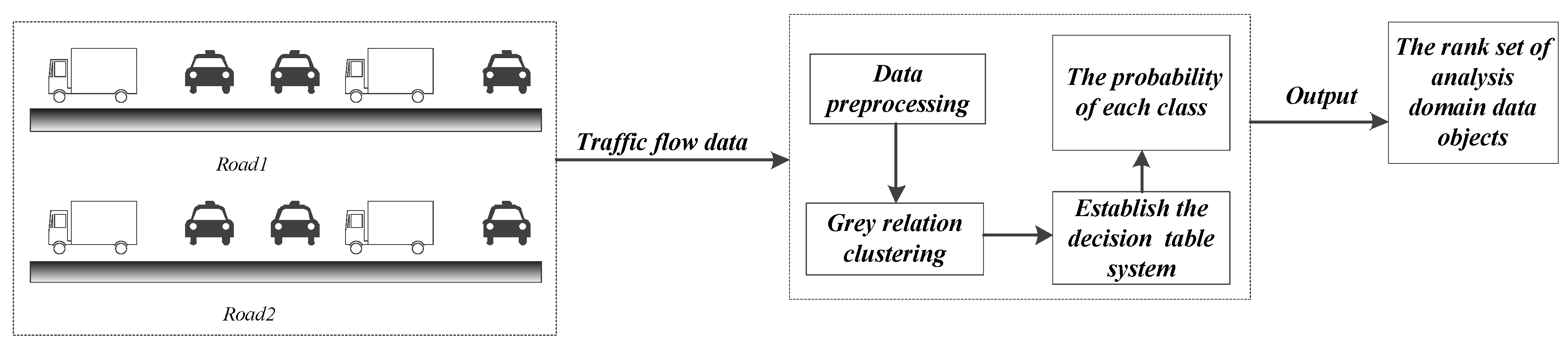
In this paper, we study the problem of multidimensional-attribute information clustering for traffic flow and propose the GMRC algorithm. First, we transform the dataset into matrix form, extract the optimal referenced standard from the dataset, and then perform the normalized processing to eliminate the effects of different units. Furthermore, we obtain the preliminary clustering results according to grey relational theory analysis. Finally, we build a decision table system to calculate the relative weight for each cluster member. The algorithm is described as follows.
- Input:
Analysis domain data set ,
Referenced array set .
- Output:
The level (rank) set of analysis domain data objects
| Algorithm 1: GMRC (X,Y) |
- 1
Level = null; Weight = null; Member = null; Entropy = null; // Initialize sets Level, Weight; Matrix Member, Entropy - 2
Data_ Preprocessing (X,Y); // Data pre-processing - 3
X0 = ExtractOptimal (X); // Extract the optimal referenced standard - 4
S = Normalization (X,Y); // Normalization processing - 5
T = MaxRelTrees (S) // Construct the maximum relational trees - 6
T’ = ClosenessTrees (T) // Construct the maximum relational tree with closeness degree - 7
Member0 = GreyCluster (X,X0); // Regard X0 as referenced standard to compute cluster member - 8
Foreach (Yi in Y) - 9
Memberi = GreyCluster (X,Yi); // Regard Yi as referenced standard to compute cluster member - 10
End - 11
F = DecisionSystem (Members); // Establish the decision table system F - 12
Entropy = CalculateEntropy (F); // Calculate the information entropy for each cluster member - 13
Weight = CalculateWeight (Entropy); // Calculate relative weights for each cluster member - 14
CalculateLevel (X); // Calculate membership degree level of Xi in X
|
The above steps of the algorithm are described as follows:
Step 1: Initialize the parameters, pre-process traffic flow data, set the threshold to filter and delete abnormal data objects (lines 1 and 2).
Step 2: According to the features of the three properties of the traffic flow data, extract the optimal referenced standard from the analysis domain data (line 3).
Step 3: Normalize the analysis domain data set in combination with the referenced standard sequences (line 4).
Step 4: Compute the grey relational degree of the corresponding matrix; further, determine the grey relational similarity matrices and then construct the maximum relational trees based on the (n + 1)th row elements of those matrices (line 5).
Step 5: Based on Step 4, construct the maximum relational tree with closeness degrees (line 6).
Step 6: Compare the closeness degree between data objects, cut off the tree when the closeness degree is less than and adjacent branches exhibit large differences, and then obtain k levels of clustering results. Similarly, we obtain in total p + 1 cluster members from the p + 1 referenced arrays (lines 7–10).
Step 7: Establish the decision table system based on p cluster members as conditional attributes obtained from the referenced standard array set. In addition, the only cluster member obtained from the optimal referenced standard (line 11) is regarded as the decisional attribute.
Step 8: Compute the information entropy of cluster members for decision making, which is used to weigh the contribution of each cluster member to the clustering results (line 12).
Step 9: Calculate the weight of each cluster member (line 13).
Step 10: Calculate the probability of each data object emerging in every clustering; then, choose the level when the probability is maximized. Furthermore, obtain the final clustering results (line 14).


