The Dual Half-Edge—A Topological Primal/Dual Data Structure and Construction Operators for Modelling and Manipulating Cell Complexes

Abstract

There is an increasing need for building models that permit interior navigation, e.g., for escape route analysis. This paper presents a non-manifold Computer-Aided Design (CAD) data structure, the dual half-edge based on the Poincaré duality that expresses both the geometric representations of individual rooms and their topological relationships. Volumes and faces are expressed as vertices and edges respectively in the dual space, permitting a model just based on the storage of primal and dual vertices and edges. Attributes may be attached to all of these entities permitting, for example, shortest path queries between specified rooms, or to the exterior. Storage costs are shown to be comparable to other non-manifold models, and construction with local Euler-type operators is demonstrated with two large university buildings. This is intended to enhance current developments in 3D Geographic Information Systems for interior and exterior city modelling.

1. GIS History

This paper presents a detailed technical description and properties of the dual half-edge (DHE) topological data structure and its application in the Geographic Information Sciences (GIS), particularly in building interior modelling. It includes associated navigation and construction operators necessary for a convenient usage of DHE. Previous papers describing DHE [1,2,3] reported on the importance of the primal/dual approach, some applications, model representation and preliminary development, but with only a brief discussion of technical details and properties. DHE is compared with some other similar data structures.

Early 2D GIS data structures were designed for polygon (choropleth) maps, where the objective was to combine the sets of individual digitized polygon boundaries to form a network. Various approaches were attempted, but finally an arc-based structure predominated, where an “arc” consisted of an intermediate set of digitized points between the “nodes” at boundary junctions. This was closely related to the winged-edge structure [4], with pointers to the four adjacent arcs and the two bounding polygons. The winged-edge structure was developed by Baumgart [4] and provided a way to connect the various edges of a two-manifold together by using a pointer-following structure. It was possible to navigate in this manner around the edges and faces of a b-rep (boundary representation) of a CAD model. From this, Mäntylä [5] developed the half-edge structure and used this to develop “Euler operators”, a set of local operations for model construction that guaranteed to preserve the topological connectivity of the model, if the input parameters were valid.

With the advent of triangulation-based terrain modelling (TINs) various methods were used to express the relationships between triangles, edges and nodes in 2D. Currently, the most commonly used are triangle-based structures and edge-based ones (winged-edges and half-edges). The Delaunay triangulation (DT) is usually used, as it has several valuable properties—in particular that it may be updated locally in expected constant time once the enclosing triangle has been found.

Its dual is the Voronoi diagram (VD), which is frequently valuable in itself as an analytic tool. If both structures are needed then a combined structure, the quad-edge [6] is frequently used. This allows navigation in the plane in either the primal or dual space, requiring only pointer references in order to follow any path in the combined graph.

More recently, GIS has gone beyond the planar view to include city models with extruded buildings, sometimes with more elaborate external structures [7]. However, these do not usually contain interior structures and, if they do model rooms and corridors, these are not topologically connected to permit indoor navigation—to provide, for example, escape route planning. For full 3D modelling with multiple volumes (e.g., building interiors, rooms), a different (new) data structure was needed. 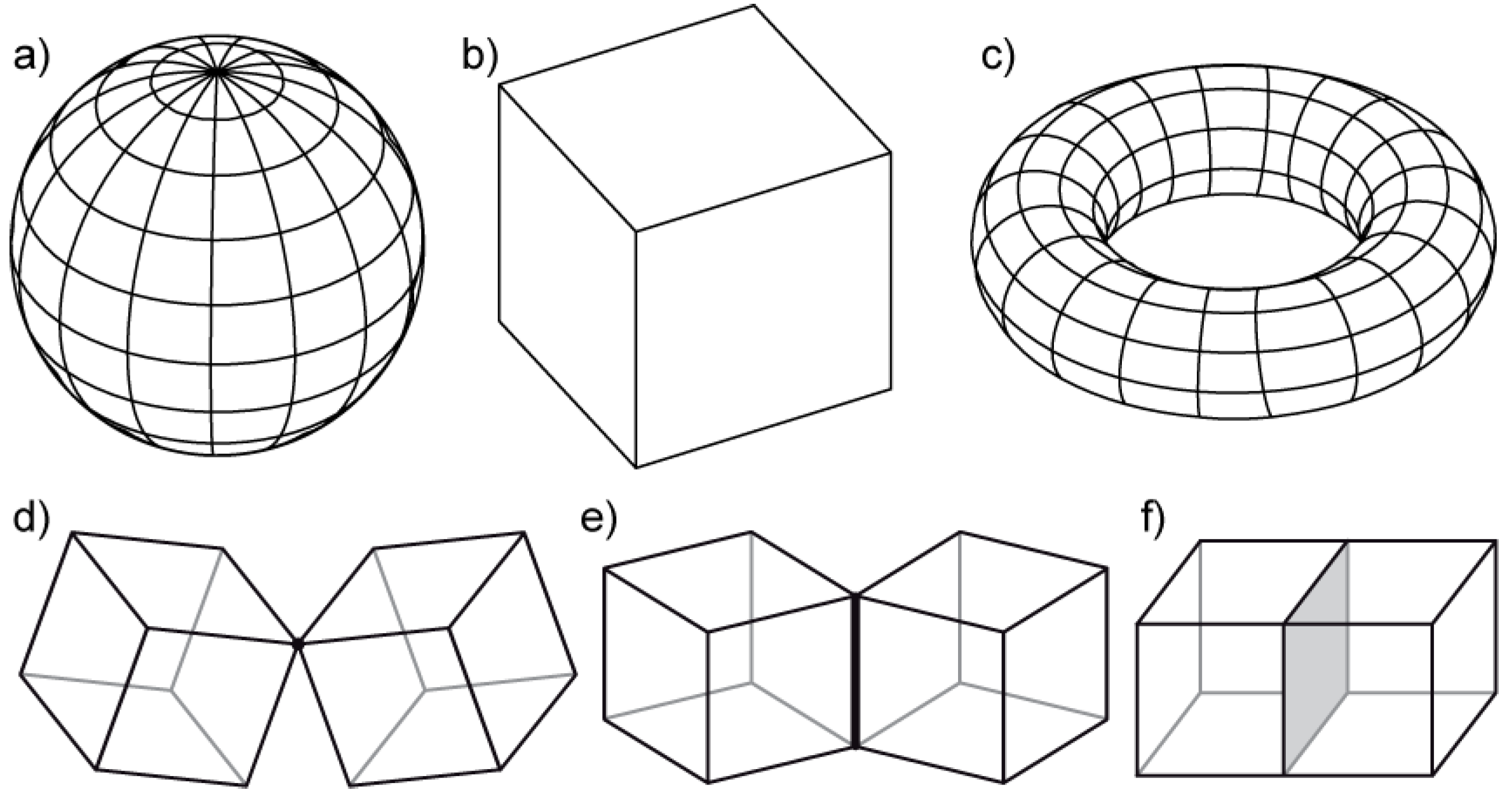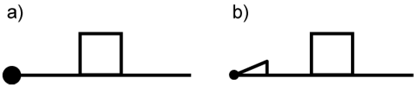Three-dimensional cell complexes were adopted as mathematical (topological) models for 3D non-manifold objects in Computational Geometry [8,9] and Computer-Aided Design [10,11]. A two-manifold is a topological space, where each point has a neighbourhood which is topologically equivalent to an open two-dimensional disk; models which do not satisfy this are non-manifold [11]. Simple two-manifold and non-manifold objects are shown in Figure 1.

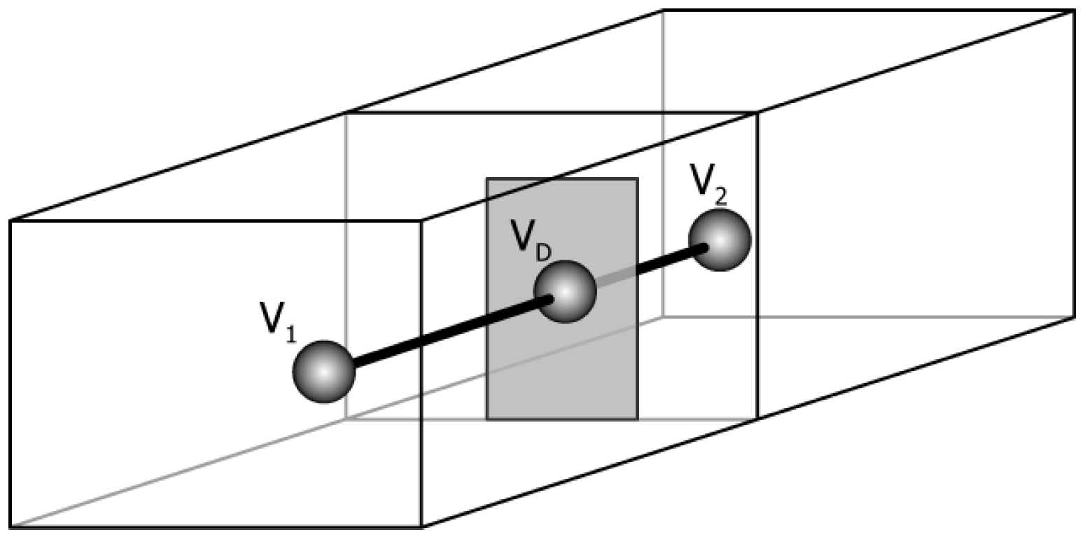
Our research objective was to extend the primal/dual concept of the quad-edge to 3D cell structures. Consideration of the Poincaré duality for the 3D VD showed that the dual of a face is a penetrating edge and the dual of a volume is a vertex—both in the primal (DT) and dual (VD) space. (In 2D, the dual of a polygon is a vertex and the dual of an edge is a “penetrating” edge.) Each 3D Voronoi cell may be constructed as a simple b-rep shell, and a pointer added to the dual edge penetrating each face. The same is true for the 3D Delaunay cell complex (Figure 2). Thus, each edge-face has a pointer to an edge-face in the dual structure—so an n-edged face has n penetrating edges in the dual, each one of these being part of the dual cell surrounding each of the n vertices of the face.

This gives the “augmented quad-edge” (AQE) structure [12,13], which uses the quad-edge (QE) data structure [6] to individually represent each polyhedron. Navigation from one Delaunay cell to the next involves going to the penetrating edge, switching to the reverse direction on that edge, and going back to the Voronoi face of the adjacent cell. Both the primal and dual cell complexes are of the same structure. Ledoux and Gold [12] showed that this structure provides navigation and construction procedures for 3D Voronoi/Delaunay structures; however, the construction is limited to adding a new vertex and associated triangular faces to the tessellation, and arbitrary 3D models and non-manifold cases are not supported.

2. The Dual Half-Edge

Although procedures allowed for the construction of the 3D VD using the AQE, it was impractical for the construction of arbitrary cell complexes such as building interiors. AQE was designed to construct tetrahedral meshes. No Euler operators or other operators were developed to manage construction of irregular shapes.

A considerable effort was invested in searching for a structure that permitted the addition or deletion of individual edges to the 3D model under construction, as well as maintaining the dual structure automatically. In addition, the structure needed to handle non-manifold cases—not only at the interior junctions of rooms, but during the construction process itself. Finally, it was realised that the problem lay with the basic structure of the quad-edge itself: the four half edges forming it needed to be separated in order to provide the atomic elements needed for construction purposes. However, separating them completely would destroy the critical primal/dual linkage, as would reverting to two matched pairs of half-edges—one in the primal and one in the dual.

The answer was to preserve pairs consisting of one primal and one (permanently linked) dual half-edge. These could be snapped together as required with other half-edge pairs to form geometric (primal) cell complexes. In this situation, all interior half-edges, in both primal and dual space, became linked to form matched pairs. However, dual edges penetrating to the exterior of the model remained unpaired. The full boundary condition could be maintained, both for the absolute boundary and for the interiors of partially or fully enclosed rooms, by adding an “exterior” set of half-edges to each new atomic element, thus giving the 3D equivalent to the 2D “make-edge” operator. The final atomic element (with complete navigation properties) consisted of four pairs of half-edges, two primal pairs connecting a pair of vertices of the model (one representing the exterior shell, and the other the interior one), and two dual pairs connecting the “interior” and “exterior” dual nodes (the first being some volume element of the model and the other either another volume element or the exterior world).

The DHE data structure is a modification of the AQE [12] to support the construction of arbitrary cell complexes. It is related to the facet-edge [9], radial-edge [14] and half-edge [5] structures. In order to provide intuitive methods of model construction and its traversal, a set of operators was developed including navigation operators, Euler operators and extended Euler operators to construct complex-based non-manifold geometric models. The technical details are fully described in [15].

The entities present in the model are: cells, faces, edges, and vertices. The cell is a 3D b-rep shell with a zero or positive volume. Note that the volume can be zero if, for example, a cell consists of two identical faces joined together by the same set of edges. A cell is bounded by faces that form a closed shell. Faces are convex or concave polygons—there is no restriction to triangle faces often utilised in GIS applications. It is assumed that the faces are planar, although non-planar faces appear at intermediate steps in the construction process. A face is bounded by edges forming a loop cycle, and edges are bounded by vertices. An edge is represented by two connected DHEs. Vertices contain unique coordinate information but no topological links.

All cells of the model are enclosed by the external cell of infinite volume. The model represents a tessellation of space, thus the external cell representing the “rest of the world” is an integral part of the model. Some of the navigation operators, developed in this research, require an adjacent cell to be present, thus the external cell needs to be present at the boundary of the model.

A similar idea of the external cell was utilized before by other researchers. Lee and Lee [10] introduced one infinite open region (equivalent of the external cell) enclosing other finite closed regions. Two-dimensional tessellation models implemented with QE [6] have the same property: internal cells are enclosed by one external cell, which is infinite; however, if the model is drawn on a 3D sphere, the external cell is a finite polygon representing the rest of the sphere surface (internal cells + external cell = sphere surface).The DHE representation has a dual nature, with complete symmetry between the two structures—the primal and dual graphs—and conforms to the 3D Poincaré duality: in either space a cell is represented by a vertex in its dual space, and a face is represented by an edge in its dual space. This reduces the construction entity types to two: vertices and edges.

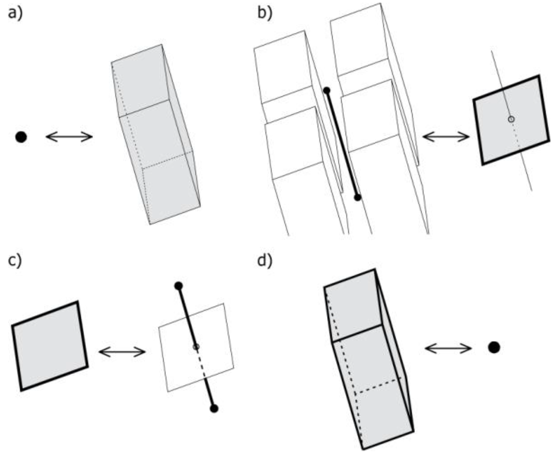
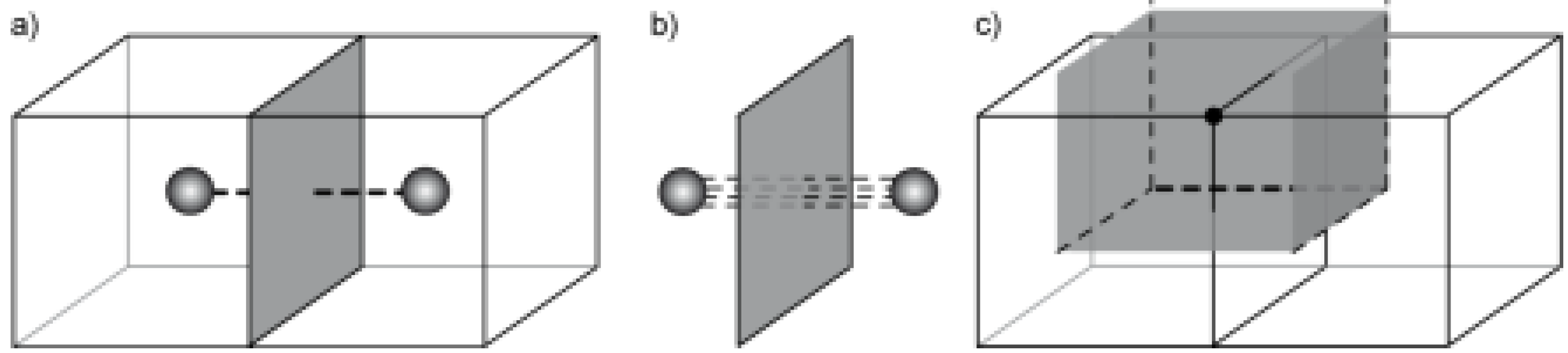
Adjacent cells of a complex are connected by a shared face, which is represented by a dual edge (Figure 3a). This edge links two dual vertices representing the adjacent cells. Technically, each face is penetrated by a bundle of dual edges—the number of dual edges is the same as the number of edges forming a face. For example, each face of a single cube cell is represented as a loop of four half-edges; each half-edge has an associate half-edge in the dual; thus, each square face is penetrated by a bundle of four half-edges in the dual (Figure 3b). Each one of these dual half-edges belongs to the dual cell surrounding one of the four vertices of the face (Figure 3c). Navigation around a bundle (radial cycle) is possible—the first step is to navigate to the dual space, then go around a face loop, and then go back to the original space. A face in terms of the Poincaré duality is represented in our model as a bundle of edges that belongs to several dual cells sharing that bundle.

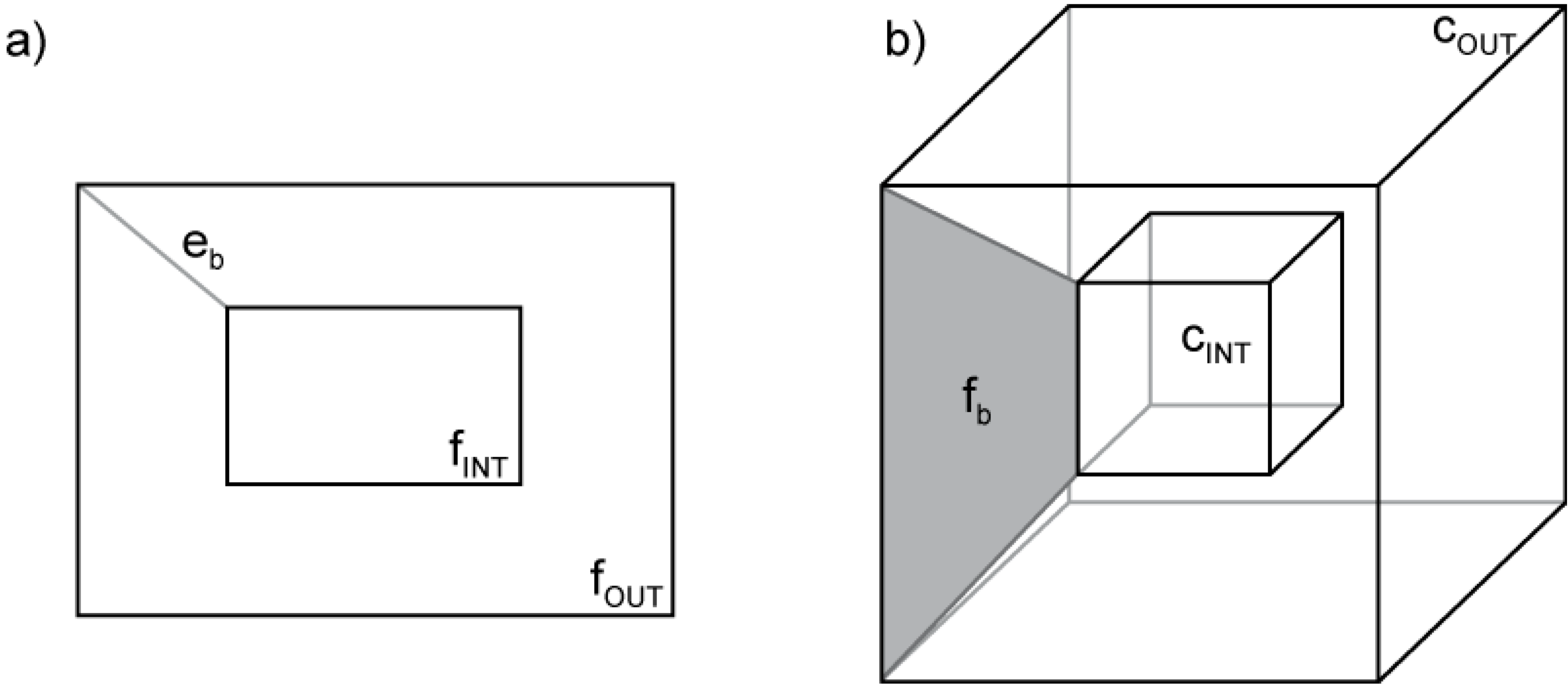
Another important property of the model is that holes and cavities are allowed: a “bridge edge” [5] (e_b in Figure 4a) is used to connect internal rings (holes) to the outside ring (the face) (f_INT and f_OUT respectively in Figure 4a); and a “bridge face” (f_b in Figure 4b) to connect an internal cell (a cavity) with the outside cell (c_INT and c_OUT, respectively, in Figure 4b). Bridge edges and bridge faces are added to a model in the same way as any others but have a special attribute that is taken into consideration by the navigation operators. This edge can be omitted during the navigation process if required. Bridge faces have the attributes assigned to their dual edges: a bridge edge in the primal graph represents a bridge face in the dual, and vice versa.

The DHE conforms to the definition of a complex-based non-manifold geometric model [11]—it allows for representation of solids where a dual node represents a volume and all primal edges and nodes connected with this node define the volume boundary; dangling faces, edges and combination of them are also possible.

2.1. Semantic Information

An important aspect of a data model in GIS is the ability to assign attributes (semantic information) to individual elements. The only construction entities kept in the DHE model are half-edges and vertices: faces and volumes are represented in the dual structure. (This holds true in either the original primal or the original dual graph.) Thus, attributes may be attached to any of these elements.

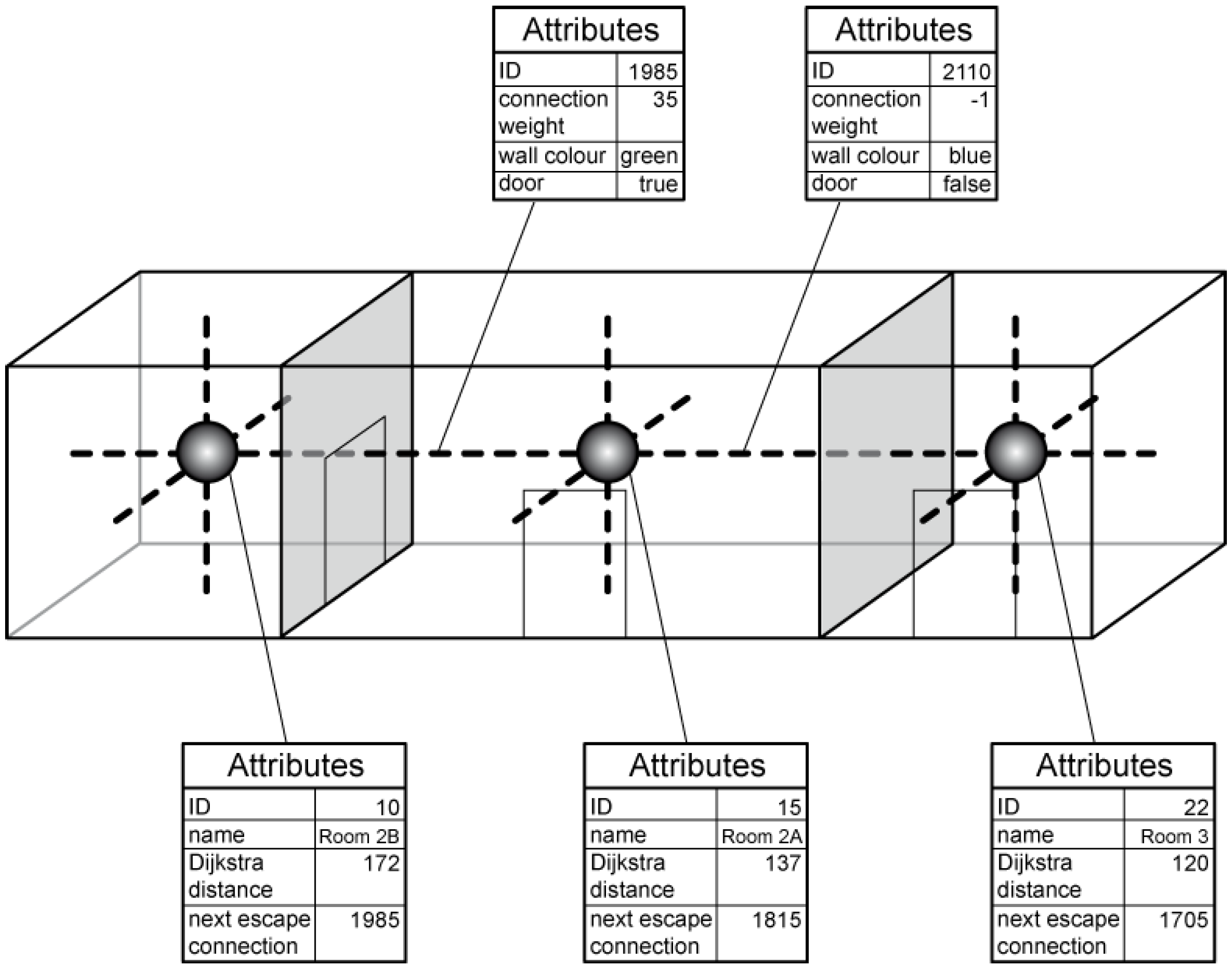
For example, in the model shown in Figure 5 there are three connected boxes representing three adjacent rooms. Rooms are represented by dual vertices, thus an attribute describing a primal cell (e.g., a room name) can be assigned to a dual vertex; two other attributes “Dijkstra distance” and “next escape connection” are used by the dual graph traversal algorithm for escape route seeking. The same idea is applied for walls and connections between rooms—a primal entity attribute can be assigned to its dual counterpart: information about wall colour or door existence can be assigned to a dual edge representing the primal wall. Because all walls are double-sided, different attributes can be assigned to each side of a wall, as they very often have different finishing. A property of a connection between rooms (e.g., “connection weight” used by a path-finding algorithm representing the cost of navigation through the connection) is a dual entity attribute, and is assigned directly to an edge connecting these rooms. Any attribute, like an ID number, can be assigned to primal and dual edges and vertices.

Because a connection between two adjacent cells is represented as a bundle of edges, an attribute can be assigned to one of the edges in the bundle and be considered as an attribute of this bundle, or a reference to the attribute can be assigned to all edges in the bundle. Bundles are directed, so different navigation weights may be assigned to each direction.

2.2. Navigation Operators

An edge is the basic construction element: half-edges are used to split an edge into two directed halves that are represented with the symbol shown in Figure 6a: a half of an edge (straight line) is associated with a face (a square in the middle) and a vertex (a dot at the end). Such an element grouping a vertex, an edge, and a face that are mutually incident is called a flag [16]. The direction is indicated by an arrow at the end associated with the vertex (Figure 6b).

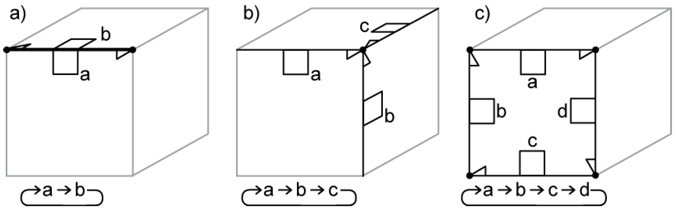
All half-edges in a model are topologically connected using pointers. Two connected halves form an edge (half-edges a and b in Figure 7a). An edge divides two adjacent faces of a cell; however, an edge can be incident to one face if a face is not planar, for example a side face of a cylinder. All half-edges in a cell sharing the same vertex are connected and form a star (half-edges a, b and c in Figure 7b). However half-edges with the same vertex from different cells are not connected directly, but they share the same vertex. Half-edges bounding a face are also connected and form a loop (half-edges a, b, c and d in Figure 7c). Each half-edge in one space is permanently linked with the half-edge in the dual—this connection made in the construction process is never modified. Half-edges in the dual are connected in the same way as in the primal.

The data structure used for the DHE representation consists of ten pointers (five to represent a half-edge in the primal and five for the dual half-edge): V, S, N_V, N_F, and D. A reference to a vertex is assigned to V. Two half-edges are joined by S. N_V and N_F are used to store information about a next half-edge in a star (around a shared vertex) and in a loop (around a face) respectively. “Next” is considered as “next” in an anticlockwise direction looking from the outside of a cell. Half-edges from the primal and dual spaces are connected by the D pointer and are set during the construction process.

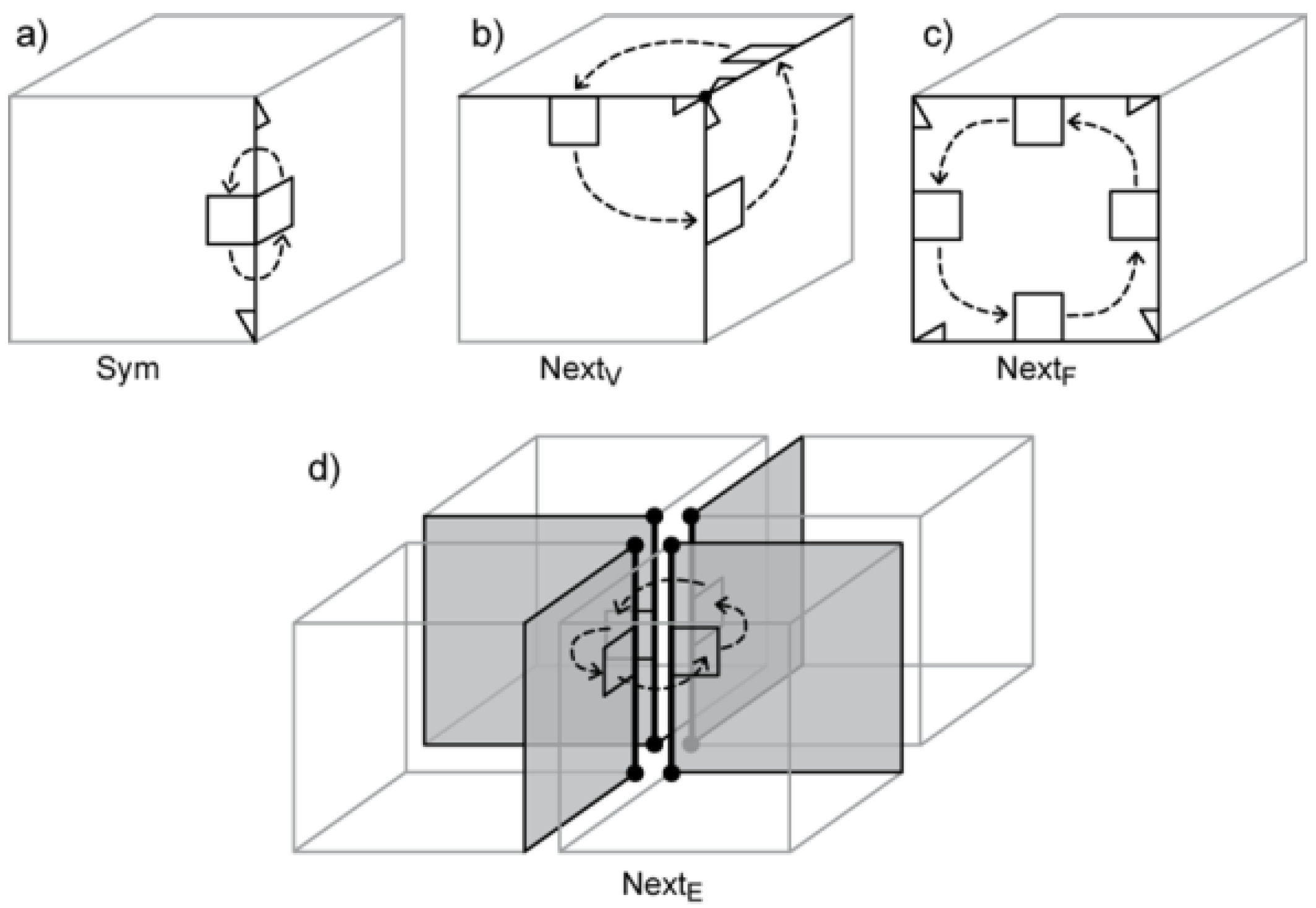
Four navigation operators use pointers directly: Sym, Next_V, Next_F, and Dual. Sym (Figure 8a) uses S to navigate from one half of the edge to the other. Next_V (Figure 8b) uses N_V to navigate around a shared vertex and Next_F (Figure 8c) uses N_F to navigate around a shared face (in both cases in the anticlockwise direction looking from the outside of a cell). Dual uses D to navigate from a half-edge in one space to the associated half-edge in the dual space.

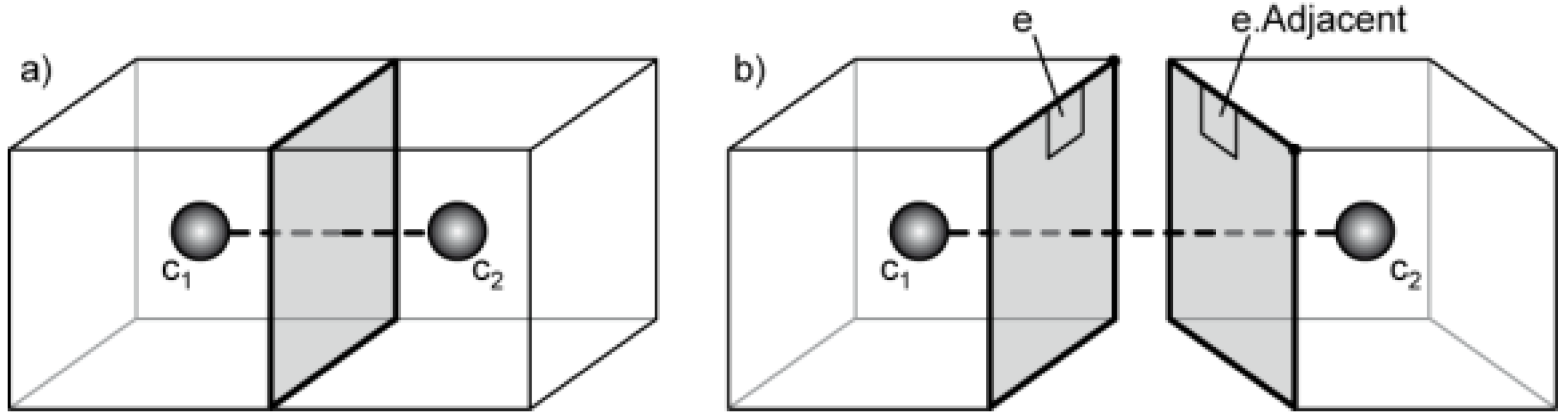
Compound navigation operators based on the basic set are also defined: Prev_V, Prev_F, Next_E, Prev_E, and Adjacent. Prev_V and Prev_F allow for navigation in the same way as their counterparts Next_V and Next_F but in the opposite direction. Next_E (see Figure 8d) and Prev_E allow for navigation around a bundle of edges. Adjacent is used to navigate to the adjacent cell—the result of the operator is an edge in the adjacent cell that has the same coordinates and is associated with the opposite side of the shared face. Figure 9a shows two adjacent cells (c₁ and c₂) that share a face. This face is double-sided—one side for each cell. The half-edge e in c₁ shown in Figure 9b is one out of four edges forming the face loop. e.Adjacent is an adjacent half-edge in c₂.

It should be noted that the aforementioned set of operators allows for navigation in both directions, CW and CCW, in models including non-manifold structures, for example, when two cells are connected by a shared node or edge. The number of pointers may be reduced in case of models, where all cells are connected by a face or the dual is not required (see Section 3.3).

Pointer notation is used here: for example, the Adjacent operator is described by a sequence: e.Adjacent = e.D.N_F.D.S, where e is the source half-edge. This should be expanded as follows: go to the dual half-edge of e, then go the next counter-clockwise half-edge around a face, then go back to the original space, and go to the opposite side of the edge.

The full set of navigation operators is described by Equations (1)–(9).

$$e.Sym\to e.S$$

(1)

$$e.Nex{t}_V\to e.N_V$$

(2)

$$e.Nex{t}_F\to e.N_F$$

(3)

$$e.Dual\to e.D$$

(4)

$$e.Pre{v}_V\to e.Dual.Nex{t}_V.Dual$$

(5)

$$e.Pre{v}_F\to e.Dual.Sym.Nex{t}_F.Dual.Sym$$

(6)

$$e.Adjacent\to e.Dual.Nex{t}_F.Dual.Sym$$

(7)

$$e.Nex{t}_E\to e.Dual.Nex{t}_F.Dual$$

(8)

$$e.Pre{v}_E\to e.Sym.Dual.Nex{t}_F.Dual.Sym$$

(9)

2.3. Construction—Euler Operators

The proposed construction of a 3D computer model represented as a cell complex allows arbitrary cells (polyhedra) of different shapes. The process of cell construction is “atomized” to make incremental construction (edge by edge) possible. This is possible with Euler operators, which are used for modifying b-rep objects as they preserve topological integrity.

Construction of a single cell (without the dual) is a simple process using traditional Euler operators. For non-manifold models it is required to be able to construct more complex structures: to create non-manifold cell complexes the standard Euler operators should be extended to manage connections between cells and to include operations like joining two cells by a shared face, edge or vertex. Extended Euler operators for non-manifold modelling including cell complexes were proposed by Masuda [11] and Masuda et al. [17].

Cells joined by a face is a normal situation in cell complex construction. Two cells can be also joined by a shared edge or vertex. In these two cases, it is not possible to navigate directly from one cell to another. However, the cells are connected via the external cell and navigation between the internal cells is possible in the dual. It should be noted that some non-manifold models can be simulated without the external cell by using the Cardboard and Tape method [1].

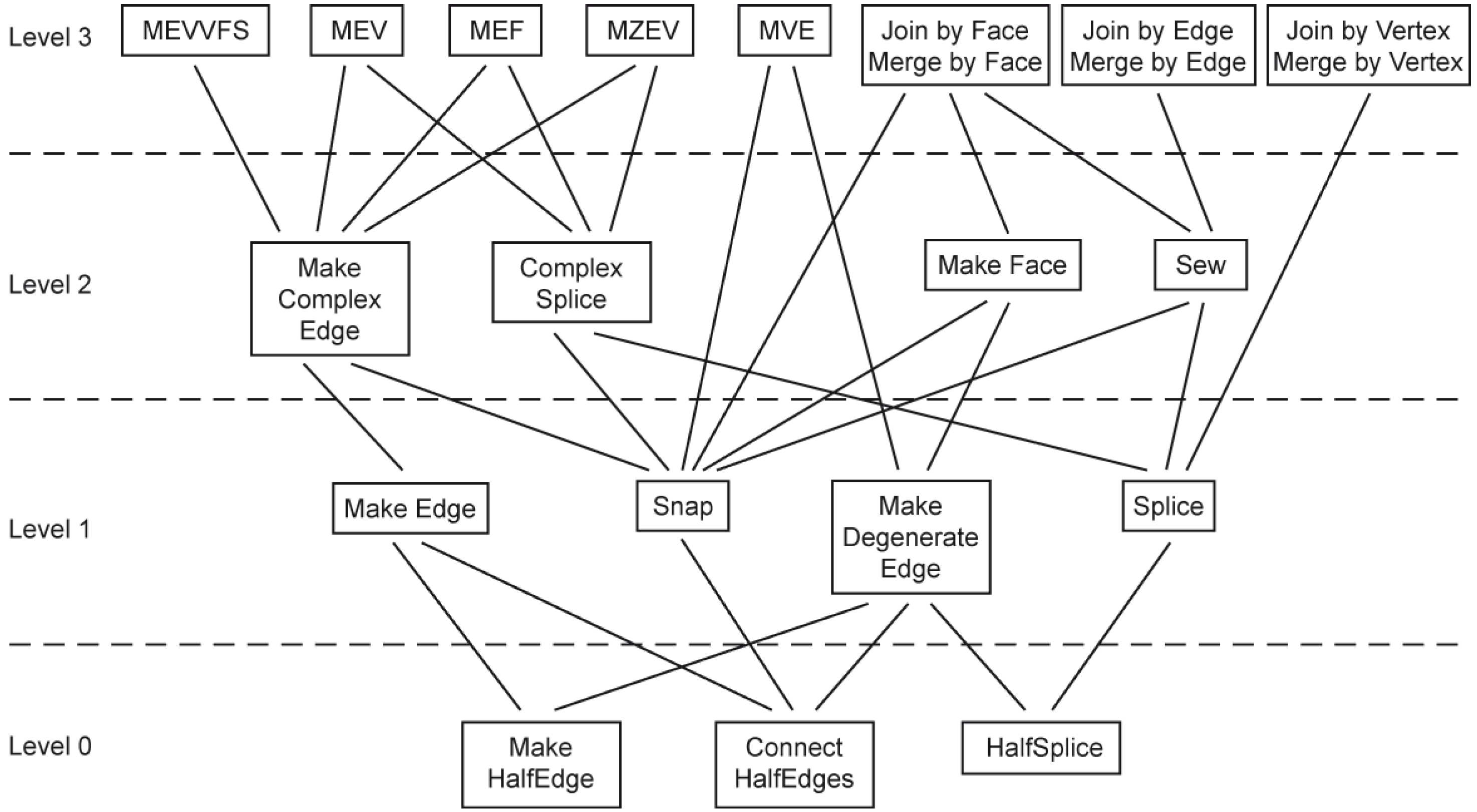
The construction operators are grouped in layers (Figure 10). Operators are dependent on operators from a lower level. Only operators from the lowest level are based on pointers and other basic operations. Operators from higher levels are more complex and specialized.

Table 1. A set of Euler operators and extended Euler operators.

Abbreviation	Operator Name
MEVVFS/KEVVFS	Make/Kill Edge, Vertex, Vertex, Face and Shell
MEV/KEV	Make/Kill Edge and Vertex
MVE/KVE	Make/Kill Vertex and Edge
MZEV/KZEV	Make/Kill Zero-length Edge and Vertex
MEF/KEF	Make/Kill Edge and Face
	Join/Separate by Face
	Join/Separate by Edge
	Join/Separate by Vertex
	Merge/Split by Face
	Merge/Split by Edge
	Merge/Split by Vertex

includes the developed operators at the highest level (level 3): Euler operators and extended Euler operators. Each pair of operators (base and reverse operators) is represented by a base operator (no reverse operators are shown in Figure 10). The full set is not covered, but a spanning set is implemented. However, there are no operators for hole and cavity construction—they are implemented using bridge edges and faces created using operators from the proposed set.

Operators from level 2 allow for construction and connection of edges (Make Complex Edge and Complex Splice) and faces (Make Face and Sew). This level may be used in applications for model construction (“Cardboard & Tape” uses Make Face and Sew).

Operators in level 1 and 0 directly change the DHE structure: operators in level 1 work with edges and call level 0 operators which work with dual half-edges: they change or assign the pointers and do not call other operators from the set. Make Half Edge is the only operator that reserves computer memory for the DHE.

Some properties of the proposed Euler operators are presented below. Lower level operators are not described here but they were introduced in this paper to show the layered idea of operator implementation.

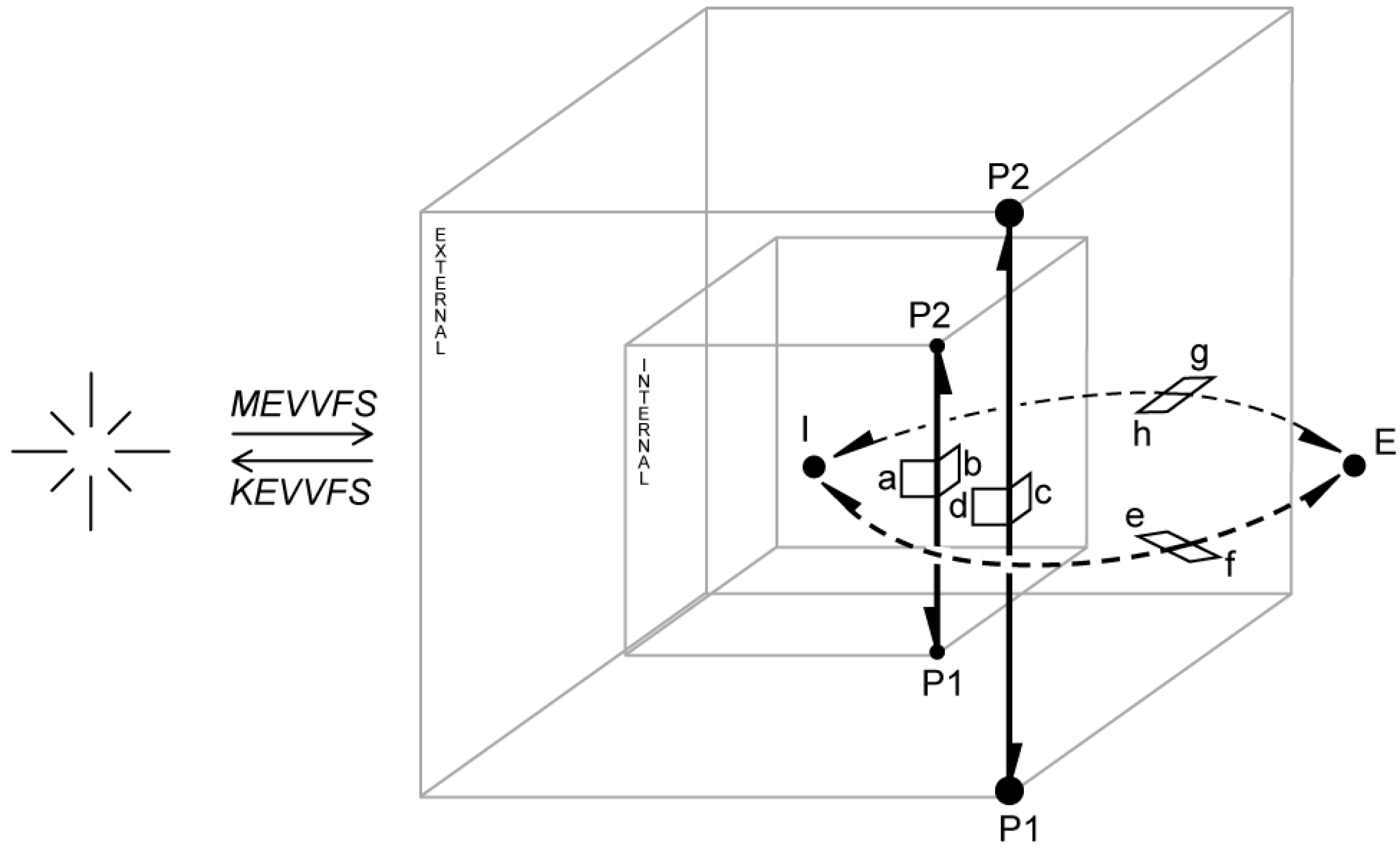
Make/Kill Edge, Vertex, Vertex, Face and Shell (MEVVFS) an operator that can be used to create a new cell (shell): a new edge in empty space is created (Figure 11). This edge forms a cell that may be further developed to obtain a polyhedron. The external cell and dual edges are also constructed. There are four edges involved in this process —two in the primal (black solid lines), and two in the dual (black dashed lines); and four vertices: two vertices in primal space (P1 and P2), and two in the dual (I and E). Vertices P1 and P2 bound a new edge. Vertices I and E are dual nodes representing the internal and external cells of a new complex—these cells are thus formed by dangling edges: the edge built of the a and b half-edges forms an internal cell associated with the I vertex; the edge built of the c and d half-edges forms an external cell associated with the E vertex. All connections set by the operator are shown in

Table 2. Table of connections made by Make/kill edge, vertex, vertex, face and shell (MEVVFS).

	S	NV	NF	D	V
a	b	a	b	e	P1
b	a	b	a	g	P2
c	d	c	d	f	P1
d	c	d	c	h	P2
e	f	e	f	a	I
f	e	f	e	c	E
g	h	g	h	b	I
h	g	h	g	d	E

: half-edges created in the process (labelled a–h) are shown in the first column, and the value of pointers (S, N_V, N_F, D and V) in other columns.

MEVVFS is not a proper Euler operator because it introduces many elements into a model: one edge, two vertices, one face and one shell (an edge is a minimal topological and valid element allowing for navigation; an isolated vertex does not bring any topological information). A face is created automatically and is a result of the DHE representation; the number of shells is determined by the number of cell complexes mutually disconnected. MEVVFS combines two standard Euler operators MFVS and MEV—see the first two construction steps in Figure 4.1 in [18].

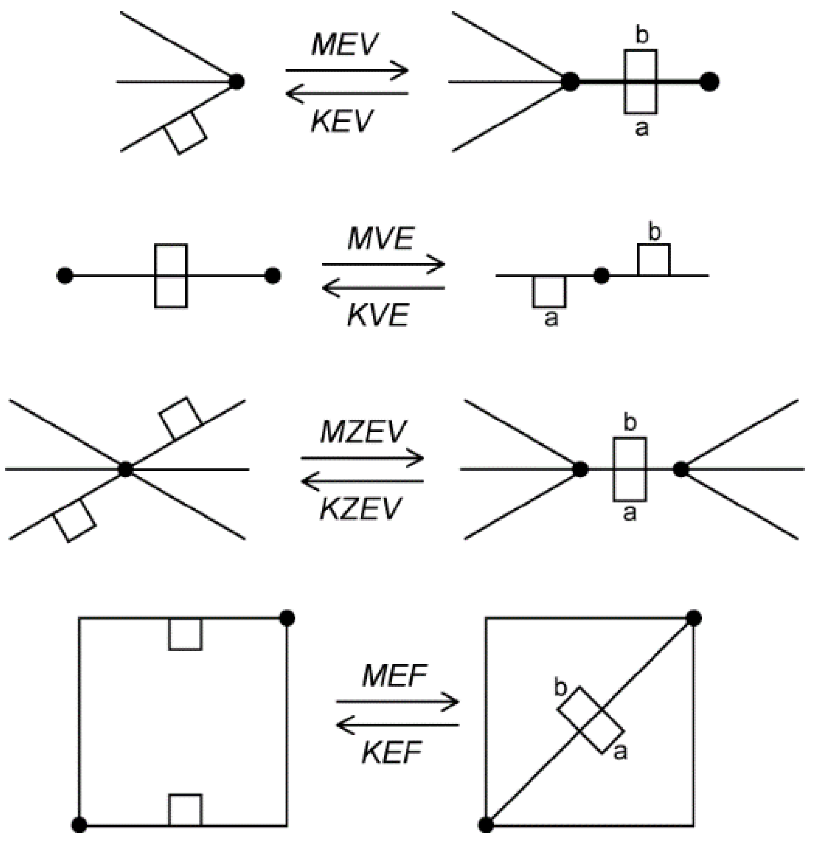
Other implemented operators (i.e., Make Edge and Vertex (MEV), Make Vertex and Edge (MVE), Make Zero-length Edge and Vertex (MZEV) and Make Edge and Face(MEF)) are considered to be standard Euler operators (Figure 12). The dual is not shown in Figure 12, but it is updated by the operators. It should be noted that some operators can be used only in the construction process of a single cell before it is added to a complex (e.g., MZEV).

Euler operators do not check if input parameters are valid. For example, usually it is expected that two half-edges from the same face loop are given as an input for MEF. The result is a new edge, which divides one face into two parts. A “strange” structure, which may be an unexpected result, is generated if two half-edges from different face loops are given as an input. For instance, if the half-edges are from different cells, the MEF operator may be used to implement additional operator MEKFS (Make Edge and Kill Face and Shell). Additional tests may be performed before an Euler operator is used in order to guarantee valid 3D cells.

It should be noted that Euler operators can create non-cellular structures as they are defined by Akleman et al. [19], for instance, a polygon with hole, with no edge between internal and outside loops. This situation can be managed by an additional level of operators, which perform topological tests and Euler operators in order to create valid cellular structures using “bridge edges”. An example which requires such a representation is an architectural model, where a window is a hole in a wall: they do not share boundaries and they may be connected by a “bridge edge”.

2.4. Extended Euler Operators

Join is a collection of three operators to connect two cells—it is possible to join cells by a common face, edge or vertex (Figure 13). The relationships between cells are changed in this way so that direct navigation between the cells is possible and the cells are part of the same complex even if they were in two different complexes before the operation. “Join” changes primal edges of the external cell; dual connections are changed automatically so that direct navigation between the cells is possible (in Figure 13 dotted lines and grey faces represent the dual). “Join” has an inverse—“Separate”.

Cell joining by a face is the most useful operator for cell complex construction. This connection is possible only if the faces have the same number of edges. They do not have to have the same vertices. However, visualization may give strange results if the faces to be connected do not fit geometrically.

In building interior modelling (the main objective in this research), escape routes and navigation between rooms is an important issue. Rooms are represented by cells. Only navigation from cell to cell through faces (doors, windows, walls, etc.) is permitted. Therefore, cells are not joined by a common edge or vertex even if they geometrically fit and such a connection is possible. However, the full set of Join operators may be important in other applications.

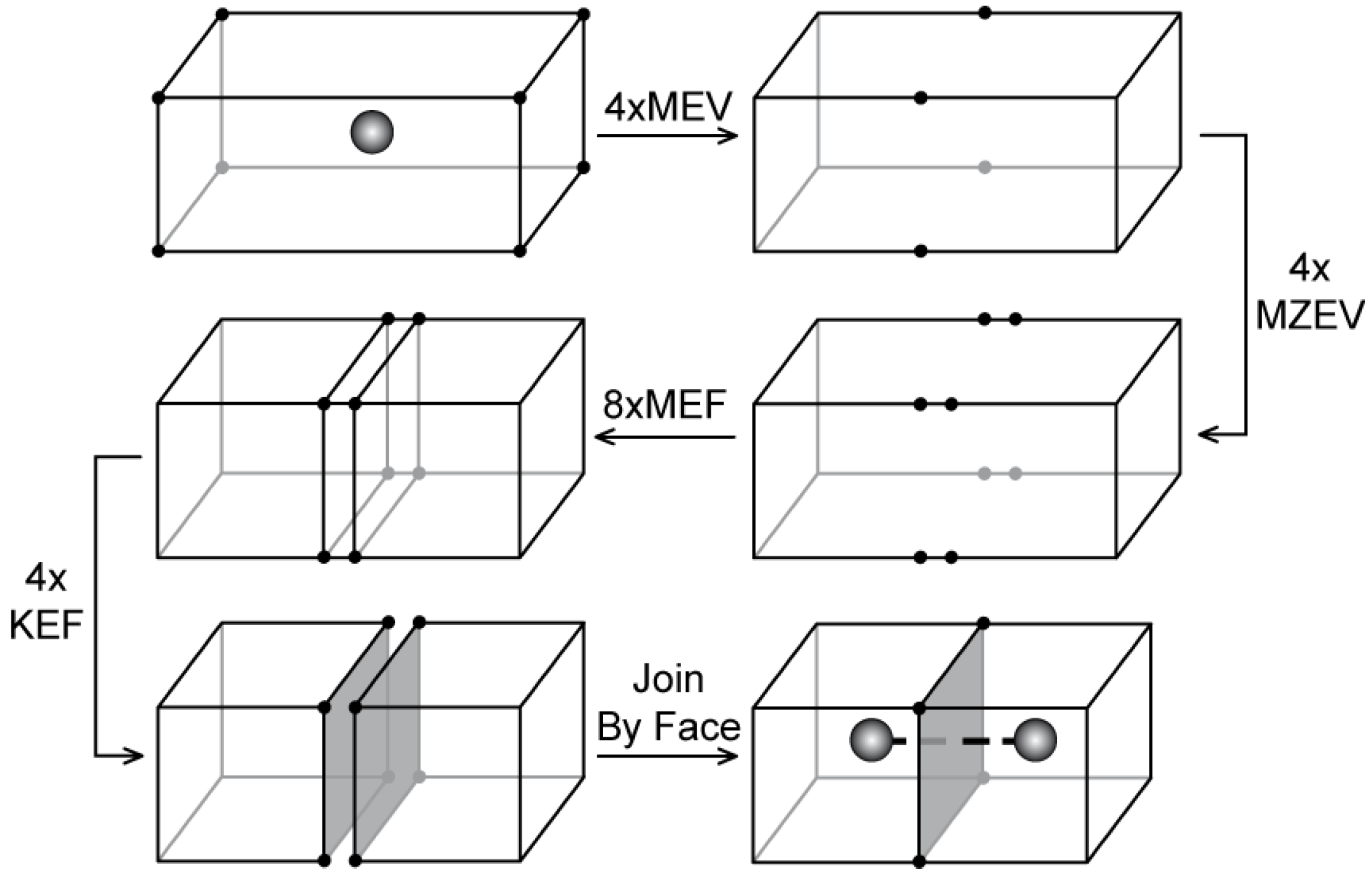
The same result (two connected cells) can be obtained in a different way (see Figure 14). This method and the set of Euler operators used is based on [20]. It should be noted that in this process the last of four KEFs before joining two cells by a face has a different meaning because with the last edge removed, the original face is split into two; the same applies to the cell. Thus, the last operator could be named KEMFS.

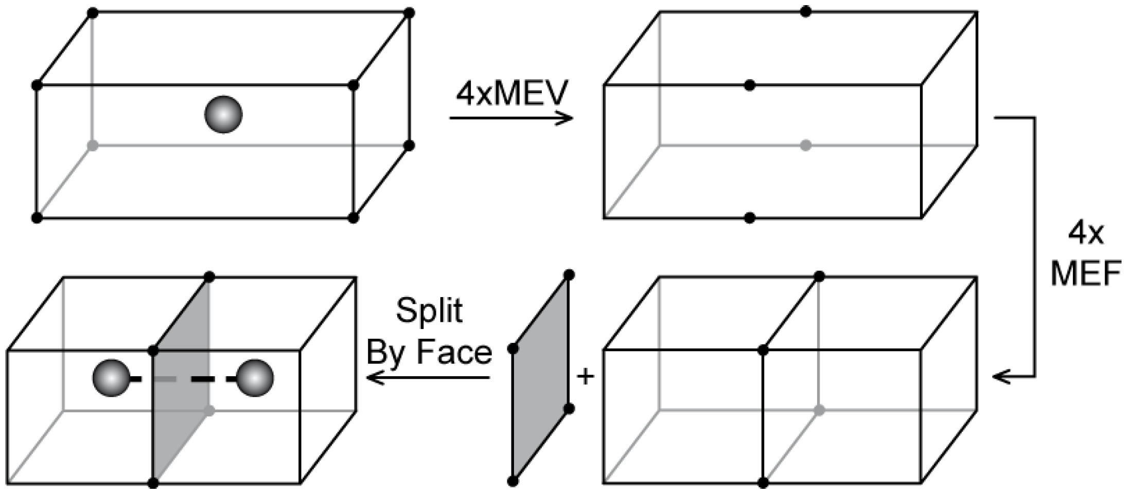
The above example can be simplified using the extended operator Split by Face (see Figure 15).

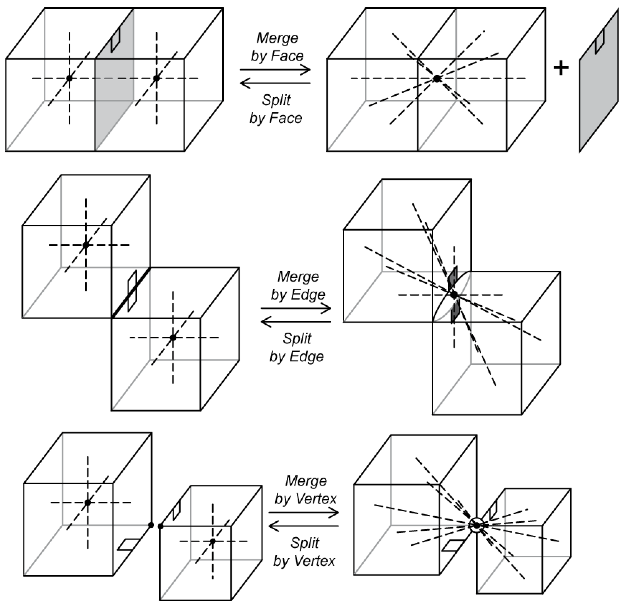
Merge, like “Join”, is a collection of three operators—it is possible to merge cells by a common face, edge or vertex (Figure 16). In this case, two cells are merged into one cell. “Merge” changes the primal edges of the internal cell. Cells to be connected have to be joined first—merging two cells that are in separate complexes has two stages: first, cells are joined, then they can be merged. “Merge” has an inverse—“Split”.

3. Comparisons with the DHE

In this section, the DHE and simplified versions are compared with other data structures. The simplified versions have a reduced number of pointers representing a half-edge. They use less storage space, but they are not able to represent all non-manifold models (only cells joined by face are allowed). In the most simplified version, the dual structure is not present, and connections between adjacent cells and attributes originally attached to dual elements are stored in the primal. Therefore, the management of semantic information may be complicated, for instance, an attribute originally attached to a dual node would have to be somehow stored in a primal cell.

The authors tried to find similar structures that are well described, and that could be used in similar applications. Three structures were selected: the coupling-entity [21,22], the radial-edge [14], and the partial-entity [10]. There are also new data structures for non-manifold modelling developed recently [23,24,25,26] but they are based on the older data structures [4,10,14,21,27,28] or else a direct comparison is difficult: they introduce many construction entities stored explicitly, like regions, shells, faces, edges, vertices, loops, disks, etc.—while there are only edges and vertices in the DHE models, similar to the feather introduced in the coupling-entity data structure.

A new spatial model recently developed in the GIS field [29,30] based on conformal geometric algebra focuses on computation of topological relations. A data structure proposed to represent the model introduces additional entities, e.g., point pairs, circles, tetrahedrons, spheres, etc., which makes the comparison with DHE even more difficult.

3.1. The Coupling-Entity—The Feather

Probably the closest CAD data structure to the proposed approach is that of Yamaguchi et al. [22] and Yamaguchi and Kimura [21]. A detailed comparison with the DHE was presented by Boguslawski and Gold [2].

A model using the feather as a basic element can be simulated with the DHE data structure. It is also possible to show that a simplified version of the DHE exists, and this is an equivalent of the feather [2]. Thus, the feather is a subset of the DHE. As a matter of fact, the simplified DHE has similar limitations to the feather: joining two cells at a shared vertex produce a model that is not valid. However, all edges sharing the same vertex can be joined in one cycle, but navigation is not valid—the inability to navigate around a face occurs. This error is caused by defining the loop cycle using the disc cycle. However, in a cell complex decomposing 3D space, where all the cells are joined by shared faces, other methods can be used to navigate between edges sharing the same vertex. A single cell in a complex is a 2-manifold, and only one disc cycle is necessary to navigate around a shared vertex. Disc cycles in other cells are not joined together, but navigation through shared faces is possible, and access to these cycles is possible.

Another difference and a big advantage in GIS over the coupling-entity is that the DHE (the full version) is able to represent a cell/volume with a single dual vertex, and a face entity with a bundle (of edges). Thus, for example, attributes may be assigned to any node, edge, face, or volume entity in either the primal or dual space.

3.2. The Radial-Edge and Partial-Entity Structure

The partial-entity structure introduced by Lee and Lee [10] is a compact data structure which is derived from the radial-edge [14]. Data storage is reduced significantly (by about 50%) without the loss of time efficiency.

In the comparison presented below, the case of a cell complex consisted of 1000 cubes (10 × 10 × 10) is used as in [10].

The total size taken by the model constructed using the radial-edge is 1,457,303 bytes, and for the partial-entity—644,192 bytes [10]; these are included in

Table 3. Storage requirements for a cell complex of 1000 cubes (10 × 10 × 10).

Data Structure (x)	Total Size	Ratio (x/RE)	Ratio (x/PE)
Radial-edge (RE) [10]	1,457,303B	100%	226%
Partial-entity (PE) [10]	644,192B	44%	100%
Full DHE	1,056,000B	72%	163%
Simplified DHE (no NF pointer) (version a)	844,800B	57%	131%
Simplified DHE (no dual) (version b)	422,400B	28%	65%

. The same restrictions are used in the calculation: the size of the field storing pointers is four bytes; fields for attributes or geometric data are not taken into consideration (only storage for topology is calculated).

The analysis is carried out for three cases: the full DHE version, and two simplified DHE versions: a) no face loops—the N_F pointer is removed; b) no dual structure—the D pointer is used to join adjacent cells.

There is one cell complex in the model: there are 1000 cubes in the complex; each cube consists of 12 edges. In the DHE, each edge is represented by two dual half-edges; each DHE contains five pointers in each space—the primal and dual (that gives ten pointers for each DHE). There is also one external cell present in the model—one big cube enclosing all internal cubes. Each face of the external cube is split into 10 × 10 grid of squares corresponding to the external faces of the internal complex—that gives 1200 edges in the external cell. Flags or lists are not used in the DHE.

For the DHE, storage space of the internal complex equals: 1000 cubes × 12 edges × 2 DHE × 10 pointers × 4 bytes = 960,000 bytes; and for the external cell: 1200 edges × 2 DHE × 10 pointers × 4 bytes = 96,000; in total 1,056,000 bytes. This score locates the full DHE structure between the radial-edge and partial-entity structures in Table 3.

3.3. Simplified DHE

It should be noted that, in the full version, the situation where two cells are joined by a vertex, and volumes (dual nodes) are stored explicitly, can be managed. However, if all cells in the analysed model are joined by faces, the simplified version without the face loop pointer N_F might be more suitable (simplified version a). The number of pointers in the DHE is decreased from ten to eight. Thus the storage space required for the model is recalculated as follows: 1000 cubes × 12 edges × 2 DHE × 8 pointers × 4 bytes = 768,000 bytes; and for the external cell: 1200 edges × 2 DHE × 8 pointers × 4 bytes = 76,800; in total 844,800 bytes. This gives a 20% space saving.

Further simplification is even less space consuming if one does not need to use volume entities. The dual structure is removed (simplified version b) and all connections between cells in the model are stored in the primal. Thus only four pointers are sufficient to store topology information. The storage space required for this case is: 1000 cubes × 12 edges × 2 DHE × 4 pointers × 4 bytes = 384,000 bytes; and for the external cell: 1200 edges × 2 DHE × 4 pointers × 4 bytes = 38,400—in total 422,400 bytes. The DHE data structure requires about 30% of the storage size of the radial-edge and 65% of the partial-entity for the cell complex representation.

Table 3 compares radial-edge, partial-entity and the three versions of the DHE. The full version with the dual graph included is useful when information needs to be stored for volumes and an explicit representation of connections between cells is important: a cell complex traversal using the dual graph is easier and the implementation of some algorithms, e.g., the Dijkstra algorithm [31], is straightforward. To save storage space, the simplified version can be used for preliminary model construction, and then this can be expanded to the full version when more advanced analysis of the model is required.

4. Building Model Construction

The resulting structure has been successfully used to reconstruct two joined buildings at the University of Glamorgan (now University of South Wales) campus. In keeping with its design objectives, it was constructed edge by edge from the original plans—faces and volumes were completed automatically when all the relevant edges were added. Euler and extended Euler operators were used which updated the dual structure in parallel. As a result, all navigation was viable at any construction stage, which simplifies the searching for the relevant portions to be attached. Finally, navigation from room to room in the dual space is readily performed by pointer-based navigation, permitting the efficient implementation of standard graph traversal algorithms, such as Dijkstra’s. The only entities preserved are the primal and dual nodes/volumes, and the primal and dual edges/faces. Any desired attributes may be attached to these, permitting a variety of intelligent searches of the overall building complex.

Rooms are not the only objects in a building that are important. Walls, doors, windows, installations. etc. are essential in many types of navigation and escape route planning and can be represented as cells with geometry and volume, and attributes can be assigned to them.

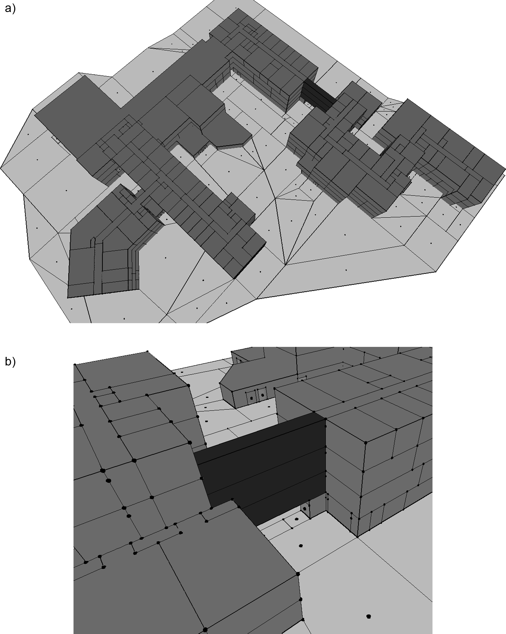
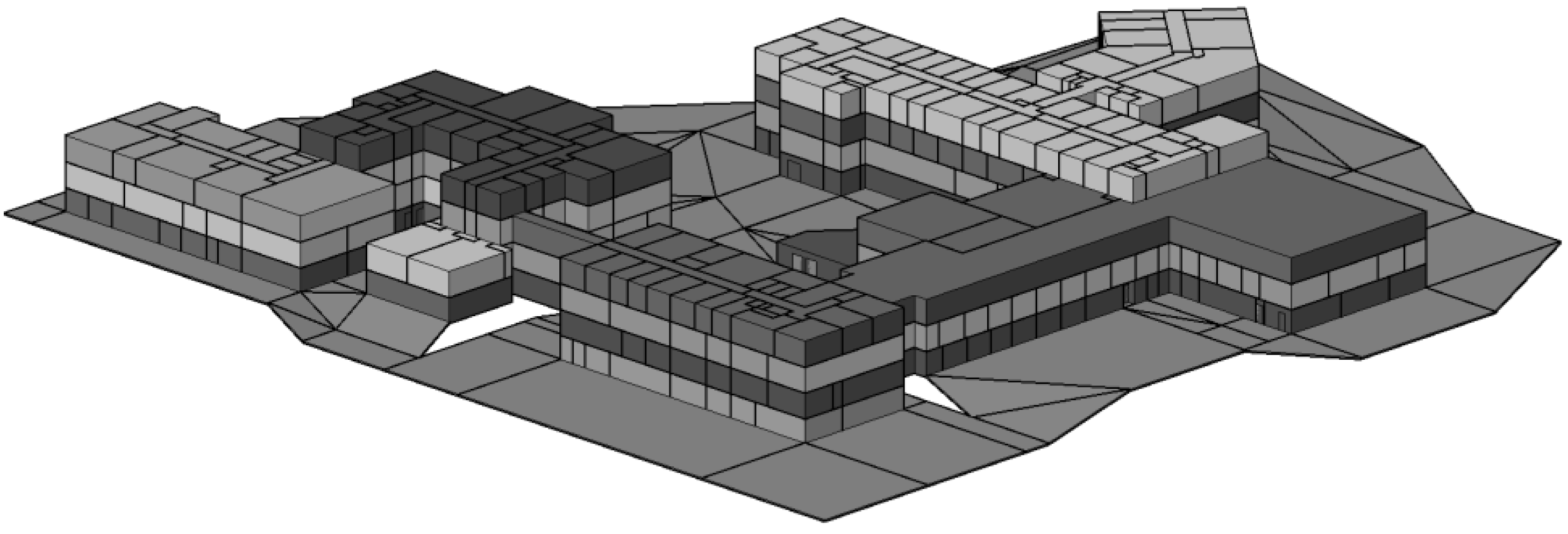
The reconstructed model—two buildings from the University of Glamorgan campus (see Figure 17a) connected by an above-ground passage (see Figure 17b)—assumes that walls have zero thickness, and may be connected by zero-thickness doors (that still have a dual node) (see Figure 18).

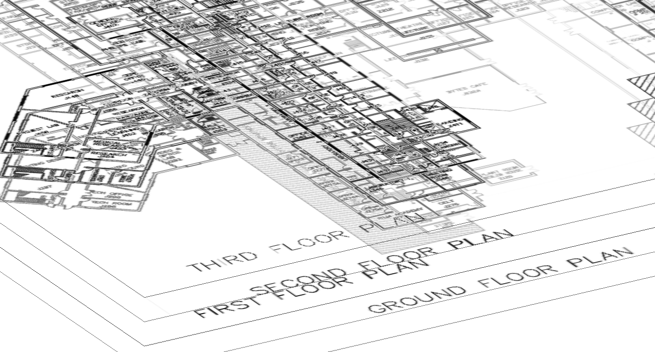
In total, there are over 1,300 cells. Cells may be rooms, doors or corridors. The model and its use for escape route planning was reconstructed from scanned paper plans. These plans were used as a raster background in AutoCAD—subsequent floors were put into layers at different heights (the distance between layers was set at an arbitrary room height) (see Figure 19). This produced a set of individual cells, one for each room but not connected together (see Figure 20). The model was imported to Autodesk 3DS Max, where labels (i.e., room number and name) were attached to each cell. The final model (still represented as a set of separate polyhedra) was exported to the OBJ exchange format, which is a geometry definition file format. All connections between adjacent rooms were set during the construction process using DHE and Euler operators, with both the primal and the dual graph being updated simultaneously. Weights were assigned to connections between rooms; they described how difficult was to move to the next room: an infinite value meant no access, any other (positive) value was calculated from the geometric distance between the dual nodes representing adjacent cells. Weights were assigned only if a door was present. Escape routes to the exterior were modelled by adding thin cells (perhaps concrete paving) to the model, allowing navigation outside the building.

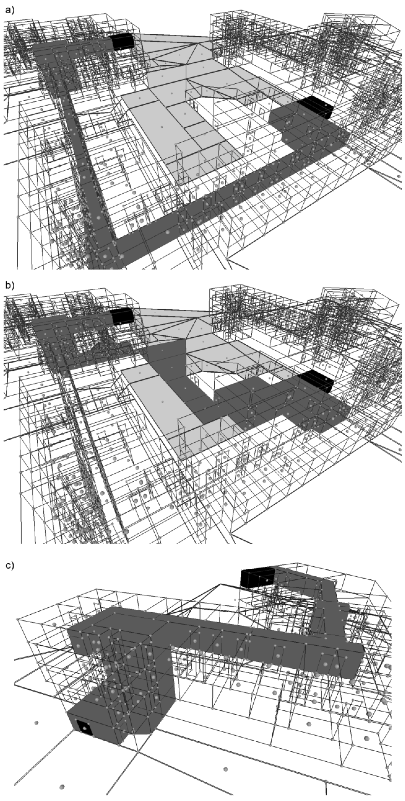
Dijkstra's algorithm was used directly on the dual graph to find the shortest path between two specified rooms (Figure 21a,b)—no additional structure was needed: a navigable network in the building is represented by the dual graph with assigned weights. The same algorithm was used to find a route from a room to the nearest exit from a building (Figure 21c)—there is one source room and multiple exits. An exit can be any cell in a complex, but usually this is a cell representing a door connecting the building with the exterior.

5. Conclusions

The novel DHE data structure shown in this paper was designed to achieve our ultimate goal. It provided a simple computer data structure to permit navigation within a cell complex, to preserve attribute information about any primal or dual entity, to permit Euler-type incremental construction and to provide straightforward tools for escape route planning.

DHE and construction operators were sufficient to build a 3D b-rep model, represented as a complex of irregular cells, using two construction entities, half-edges and nodes, while representation of volumes, faces, edges and vertices was provided by a full implementation of 3D Poincaré duality. Model construction, based on Euler operators, includes automatic updates of the dual representing the logical structure of the model. The only element used for topological connections was a half-edge, while a node was used only to store the coordinates of a vertex. Attributes could be attached either to half-edges or nodes. These properties meet the requirements for GIS models where integration of geometry, topology and semantics is crucial.

It should be noted that Euler and extended Euler operators do not guarantee that provided input parameters will result in a correct shell. For example, if two half-edges from different face loops are given as an input for MEF, the result will be different than a face split into two parts, which is the anticipated result. Some operators, e.g., JoinByEdge, may produce non-orientable two-manifolds, such as the Möbius strip, which may not be an expected result in a cell complex construction. A higher level of operators may be developed in order to check the correctness of input parameters and to call the right operator. In addition, new specialized operators might be required for specific applications, such as architectural modelling.

It was shown that storage efficiency of DHE is comparable with other non-manifold CAD structures, and several simplified versions have been proposed where full navigation of all possible topological adjacency types (e.g., vertex to vertex only) are not required. In this research, the focus was put on storage requirements, because topological data structures are usually memory consuming. In return, topological queries are faster due to the topological connections being included in the data structure. Comparative performance analysis will be considered in future work.

The presented DHE data structure is suited for full 3D models. However, its potential is much bigger, and it has already triggered new research. It was shown that 2D/3D integration between the 3D building interior and 2D external terrain is viable [32]. A new concept of a modified DHE, dual half-arc, was introduced by Anton et al. [33].

A simple method for escape route finding presented in this paper is to show applicability of the model for indoor navigation. The method is based on a network representing a logical structure of a building. In a general scenario working for any building, it may be necessary to partition corridors and calculate a detailed navigable network in order to get more accurate results. Such an attempt was made in [34].

Within the GIS world, there is considerable interest in the automatic generalisation of building models for representation at different scales. This has not been attempted here but is being considered for future work. Finally, no validation tools, to check the reasonableness of the geometry, have been attempted—again discussion is underway for future work. However, an attempt to validate building information models using DHE was done by Kraft and Huhnt [35].