Article

Towards Automatic and Topologically Consistent 3D Regional Geological Modeling from Boundaries and Attitudes

1
College of Resources and Civil Engineering, Northeastern University, Shenyang 110819, China
2
School of Environmental Science and Spatial Information, China University of Mine & Technology, Xuzhou 221008, China
3
Development and Research Center of China Geological Survey, Beijing 100037, China
*
Author to whom correspondence should be addressed.
ISPRS Int. J. Geo-Inf. 2016, 5(2), 17; https://doi.org/10.3390/ijgi5020017
Submission received: 21 September 2015 / Revised: 6 January 2016 / Accepted: 5 February 2016 / Published: 17 February 2016
(This article belongs to the Special Issue Multi-Dimensional Spatial Data Modeling)

Abstract

:
Three-dimensional (3D) geological models are important representations of the results of regional geological surveys. However, the process of constructing 3D geological models from two-dimensional (2D) geological elements remains difficult and is not necessarily robust. This paper proposes a method of migrating from 2D elements to 3D models. First, the geological interfaces were constructed using the Hermite Radial Basis Function (HRBF) to interpolate the boundaries and attitude data. Then, the subsurface geological bodies were extracted from the spatial map area using the Boolean method between the HRBF surface and the fundamental body. Finally, the top surfaces of the geological bodies were constructed by coupling the geological boundaries to digital elevation models. Based on this workflow, a prototype system was developed, and typical geological structures (e.g., folds, faults, and strata) were simulated. Geological modes were constructed through this workflow based on realistic regional geological survey data. The model construction process was rapid, and the resulting models accorded with the constraints of the original data. This method could also be used in other fields of study, including mining geology and urban geotechnical investigations.

1. Introduction

Regional geological survey is the systematic investigation of the geological and mining condition in the target area. The primary mission of geological survey is to investigate and expound the attitudes, distribution, components, ages and mutual relations of the geological bodies (strata and rock), build the regional geological map databases and provide fundamental data for the infrastructure construction through geological theories (e.g., geology, geophysics, and geochemistry) as well as the digital mapping technology. Geological maps and section maps are the traditional expression methods of the geological survey results. However, it is very difficult to imagine and understand the underground development of the geological bodies through the 2D geological maps. With the development of computer graphics and 3D modeling technology, 3D geological mapping was carried out in the developed countries over the past two decades, including USA [1], France [2], UK [3] and German [4]. The modeling results were applied to seismic hazard evaluation [5], geological statistical analysis [6], groundwater assessment [7], Geophysical inversion modeling [8] and geothermal exploration [9]. Some countries have released the results on the Internet. Unfortunately, the transformation from 2D maps to 3D models remains difficult and time-consuming.
Traditional 3D geological construction is mostly manual modeling based on drill-holes [10,11,12] and cross-sections [13,14] with many manual interactions. The large workload and low efficiency associated with working with large study areas and datasets are usually problematic for geological staff. Based on the experience of the British Geological Survey (BGS) in producing 1:50,000-scale 3D geological maps in GSI3D software by integrating topographic maps, drill-hole data, geological maps and other data, the 3D modeling efficiency can be less than two square kilometers per day [3]. Nowadays, the nationwide 1:50,000 regional geological surveys are being carried out in China. The modeling data that can be acquired generally are 2D geological maps containing attitudes, boundaries and route sections. This paper focuses on the issue of how to construct the corresponding 3D regional geological model based on these data to provide assistance for the mineral prospecting and geological hazard forecast.
The goal of this work was to develop a method for the rapid, topologically consistent and automatic creation of regional 3D geological models. The construction process was divided into two parts: underground modeling and top surfaces modeling. First, the geological boundaries were used to construct the geological interfaces between the bodies under the constraint of attitudes using the Hermite Radial Basis Function (HRBF) implicit method. The underground parts of the geological bodies were then developed using the face-body Boolean method between the interfaces and the fundamental body of the map area. Finally, the top geological surfaces were constructed by coupling the boundaries with digital elevation models (DEMs).
The remainder of this paper is organized as follows. Section 2 presents related studies. In Section 3, we introduce the modeling elements used in this study. Section 4 presents the workflow of our modeling method. Section 5 explains the method of constructing the top surfaces of the bodies. Section 6 discusses the main method of extracting the geological models from the subsurface of the map area. We describe several algorithms that can be used to intersect the HRBF surface with lines and triangles in Section 7. In Section 8, we present the results and the analysis of the modeling experiments. Finally, in Section 9 we conclude and anticipate the direction of future work.

2. Related Work

Geological maps are the most important results of geological surveys. To satisfy the demand for the representation of deep geological information, it is usually necessary to extend single-layer 2D maps to 3D models [15]. In contrast to typical engineering objects, the complex geometries and topologies and the scale dependency and hierarchical relationships involved in such work make traditional CAD systems unsuitable for complex geological modeling. Thus, there is an urgent need to develop specific geological modeling systems that can be used to create geological models [16,17].
3D computer modeling methods can be generally classified into two types according to the geometric characteristics of target objects, including: regular-body modeling and irregular-body modeling. Regular-body modeling method is usually used in the computer aided design (CAD), such as CSG and Voxel [18]. Mechanical parts [19] and buildings [20] are usually modeled by the regular-body modeling method. Meanwhile, to construct smooth 3D models, numerous methods have been developed for the construction of surfaces based on interpolation of values and gradients. The partial differential equation (PDE) surface proposed by Bloor et al. can interpolate constraint data to construct a smooth surface [21]. Carr et al. interpolated sparse points using a radial basis function to obtain an implicit surface using hand-tuned offset points to find a non-trivial interpolant [22]. To avoid offset points, Macedo et al. [23] proposed using the HRBF to directly interpolate the values and the normal. These surfaces have been widely used in CAD/CAM and have made surface modeling much simpler.
The surface modeling technology can construct complex spatial surface and is suitable to describe the natural structures with irregular shapes and complex inner attributes. As a consequence, it was applied into the 3D geological modeling. In recent years, the implicit surface modeling has especially been paid much attention. It has been improved so it can be adjusted to geological data, for example, by the use of Eigen analysis to simulate folds [24,25]. We regret to say, however, that only structural surfaces were constructed without specific geological bodies. The idea of using implicit surface to delineate basic geological outlines was also used to construct the geological interfaces [17,26] and to extract basic geological bodies. These proposed methods simulate geological bodies accurately but have not been used to construct large-scale 3D geological maps. In addition, the modeling methods are not efficient enough, and the models cannot pass through the control points.
The advantages of the implicit method have also attracted professional software companies, and some geological modeling software packages, such as Leapfrog [27,28], Micro Mine [29], and Vulcan [30], have provided radial basis function modeling packages. These user-friendly and efficient 3D modeling platforms enable convenient construction of geological models [31]. However, these platforms focus mainly on drill-hole datasets, and their use in geological survey modeling is challenging.
With the development of 3D geological modeling methods, some novel modeling methods have been proposed based on the geological attributes, including potential-field interpolation, stochastic and uncertainty method. The regional 3D geological models [32], as well as fundamental structures have been simulated by these methods, including folds, faults [33], reservoir structure inverted from dynamic fluid flow response [34], domes [35], and multilayered structures. Some software packages, such as the TProGS package, produce stochastic geological realizations through Sequential Indicator Simulation [36]. These are very novel methods, and their application in large-scale geological mapping remains not fully developed. We should consider not only the validity of one body but also the consistency of all of the geological bodies; that is, we should use topologically consistent models. To construct topologically consistent models in the CAD field, the Boolean method is commonly used [37]. In this paper, the Boolean idea was used to ensure that there were no seams between the adjacent models. The models should also fully satisfy the constraints of the measured data. Thus, automatically constructing geological models with the same topology using the strong constraints of multi-source data is a significant challenge in 3D geological modeling.

3. Modeling Elements

Geological maps are usually constructed using attitudes and boundaries as well as the properties stored in the backend database. In addition, section maps that describe the underground spatial forms of the geological bodies are also usually provided. The geological boundaries represent the spatial distribution and contacts of the geological bodies. The combination of all attitudes and boundaries provide the spatial shapes of the geological interfaces. Therefore, through these two geological survey elements and digital elevation model data, the geological models are mainly represented. This paper focuses on geological modeling constrained by these types of geological survey data.

3.1. Attitudes

Attitudes describe the spatial characteristics of geological surfaces, including their direction and degree of inclination. In contrast to cross-sections or drill-holes, attitudes are measured near the boundaries, and the attitudes describe the spatial form of the nearby interfaces. A single attitude can represent the approximate shape of a geological interface. Attitude is described by dip direction and dip angle. The dip direction and dip angle can be used to transform the attitude into a vector, which is called an attitude vector. The attitude vector is the direction that a drop of water would follow if it fell on the surface. The cross product of the attitude vector and the boundary’s tangent vector is the normal vector of the surface, which is the mathematical gradient of the surface.

3.2. Boundaries

Geological bodies are buried in the ground or extend to the surface; for those that extend to the surface, the intersection line of a geological body with the surface is the geological boundary. As very important elements of a geological map, boundaries display spatial distribution, topological relationships and the basic form of the geological bodies; as a consequence, they are treated in this paper as the strongest constraints for 3D geological modeling. The outcrops of the bodies and the contact relationships are expressed by the boundaries. The boundaries between conformable strata are nearly parallel, and those of unconformable strata intersect with other boundaries. The geological boundaries are all organized as a formal data structure (FDS) [38]. When a geological boundary intersects other boundaries, the segmented arcs that make up the boundaries terminate at the intersection points, and the interfaces also terminate. It is clear that the outcrops of the interface were a series of arcs, which were chosen to construct the interface. Thus, after all the arcs were applied to the extraction operation, the 3D models’ topology was consistent with the boundaries’ topology.

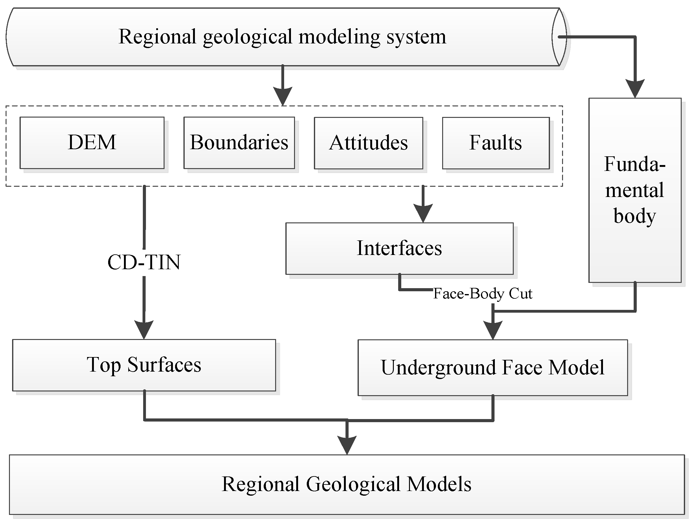
4. Modeling Workflow

Based on the regional geological survey workflow and the chronological sequence of the geological bodies, the workflow (Figure 1) for constructing geological bodies was designed as follows:
(1)
The upper surfaces were constructed from a constrained Delaunay triangulated irregular network (CD-TIN) by coupling the geological boundaries and the DEMs [39,40].
(2)
A fundamental body that contains all of the regional geological bodies was constructed.
(3)
Using the attitude constraints, the geological interfaces were constructed from the geological boundaries’ arcs.
(4)
Using face-body Boolean calculation, the geological bodies were extracted from the fundamental body.
(5)
The top surfaces of the geological bodies were matched to the surface entities that were created in step 4 through their boundaries.

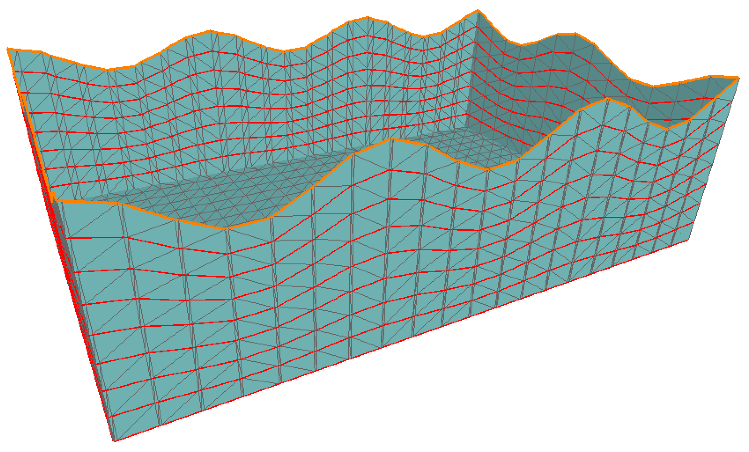
5. Top Surface Models

The geological boundaries determine the extents of the geological bodies extending to the surface, and the DEM describes the terrain in the region of interest. Neither of these elements can be ignored when constructing the bodies’ top surfaces. The constrained Delaunay triangulation algorithm was used to couple the boundaries, and the DEM was used to construct the top surfaces (Figure 2). The general process was as follows:
(1)
A triangulated irregular network (TIN) was constructed from the DEM points and the points along the boundaries.
(2)
The boundary was substituted into the TIN model, and the triangles that intersected the boundary were constructed until they were distributed on both sides of the boundary.
(3)
The triangles above the body’s top surface were deleted, and the top surface was acquired.

6. HRBF Body-Extraction Method

In Section 3, we described how the attitudes could be transformed into the gradients of the geological interface. Taking into consideration that the boundaries are the outputs of the interfaces, it is clear that we need only find a method to interpolate the values and gradients; for this, the HRBF implicit surface is a good choice. This interpolation method is highly accurate, but only an implicit function is acquired from the values and the gradients. To obtain the triangular meshes, marching cubes or marching tetrahedrons have been used to approximately model the surface [18]. However, these two methods are only interpolation methods; thus, the surface model cannot pass through the boundary points without being changed. At the same time, the boundary points are connected to obtain the boundary polygon, which makes it impossible for the surface to conform exactly to the geological boundaries. In addition, Boolean calculation between two triangular meshes is complex and inefficient. To improve the accuracy and efficiency, the implicit polygonization and Boolean methods were modified here.

6.1. HRBF Interfaces

Based on the values and gradients, a function surface can be acquired using HRBF interpolation [19]. The HRBF implicit surface is highly accurate and smooth, and the function values of the control points are 0, which means that the function can pass through the control points without any deviation. In this method, all of the control points were considered to be Hermite centers, and an implicit function was constructed to interpolate all of these points. The interpolation function has the form
f ( x ) = i = 1 n ( α i φ ( x x i ) β i , φ ( x x i ) )
where φ ( x ) = ( | | x | | ) is the radial basis function (in this paper, the global support radial basis function ( t ) = t 3 ) and α i R , β i R 3 are unknowns and can be uniquely determined by the coordinates and gradients of the boundary points. The equations used to calculate these unknowns are
{ f ( x j ) = i = 1 n ( α i φ ( x j x i ) β i , φ ( x j x i ) ) = 0 f ( x j ) = i = 1 n ( α i φ ( x j x i ) H φ ( x j x i ) β i ) = n j
where H is the Hess operator:
H = [ 2 x x 2 x y 2 x z 2 y x 2 y y 2 y z 2 z x 2 z y 2 z z ]
The equations can be transformed as
A λ = c
where A is a 4n × 4n matrix and λ and c are 4n vectors. In this method, n points provide 4n equations and 4n unknowns. Through the inverse matrix of A, λ can be calculated as
λ = A 1 c
The HRBF implicit surface’s parameters were then acquired, and the surface was uniquely determined.

6.2. Fundamental Model

The first step in extracting the model of the geological bodies from the map area was to construct a fundamental model that contained all of the geological bodies. Because the top surfaces of the geological bodies were the coupled models of the boundaries and the DEM and because the DEM was too large, the fundamental body did not have a top surface. In addition, to force the geological interface to pass through the geological boundaries, these interfaces were constructed not by the Boolean calculation but by using the method proposed below. Thus, the fundamental body was not a body model but rather a face model, which only provided the most primitive side and bottom surfaces of all of the bodies. Any bodies that were extracted from the fundamental body were only surface models without top surfaces.
Because the fundamental model included only the side and bottom faces of the bodies, we constructed the model from the boundary polygon of the map area. Two parameters—the model’s bottom altitude and the grid distance—were first specified. These two parameters determined the minimum elevation of the bodies and the modeling precision. According to the grid distance, the boundary polygon was extended downward to the modeling elevation layer by layer. The adjacent layers of the polygons were connected to construct the side surface [41]. The grid points inside the bottom boundary polygon were then chosen from the bottom polygon and the grid distance. The bottom surface of the fundamental body was constructed as a constrained triangulation network that coupled the grid points and the bottom polygon (Figure 3). At this point, the fundamental body was complete and contained all of the geological bodies.

6.3. Face-Body Boolean

To force the interface to pass through the boundary and improve the modeling efficiency, completely new Boolean and implicit surface polygonization methods are proposed here. Using the method of intersecting triangles with the implicit surface introduced in Section 7, the triangles were divided into two parts on both sides of the surface. In this process, any triangles that intersected the implicit surface formed an intersection line, and all of the intersection lines were connected as an open polyline. This polyline and the boundaries’ arcs that were chosen to construct the geological interface were combined as a polygon that corresponded to the spatial extent of the interface.
Because the constructed interfaces did not overlap vertically, which meant that the interface was only a 2.5-dimensional surface, the interface was constructed using the constrained TIN method. Using a series of plumb scanning lines inside the range polygon, the intersection points of these scanning lines and the implicit surface formed the sampling points of the surface. The constrained triangulation network generated by coupling these sampling points and the range polygon formed the interface model. The Boolean calculation was then completed, and the fundamental model was divided into two models (Figure 4); thus, a new geological model was extracted from the fundamental model.

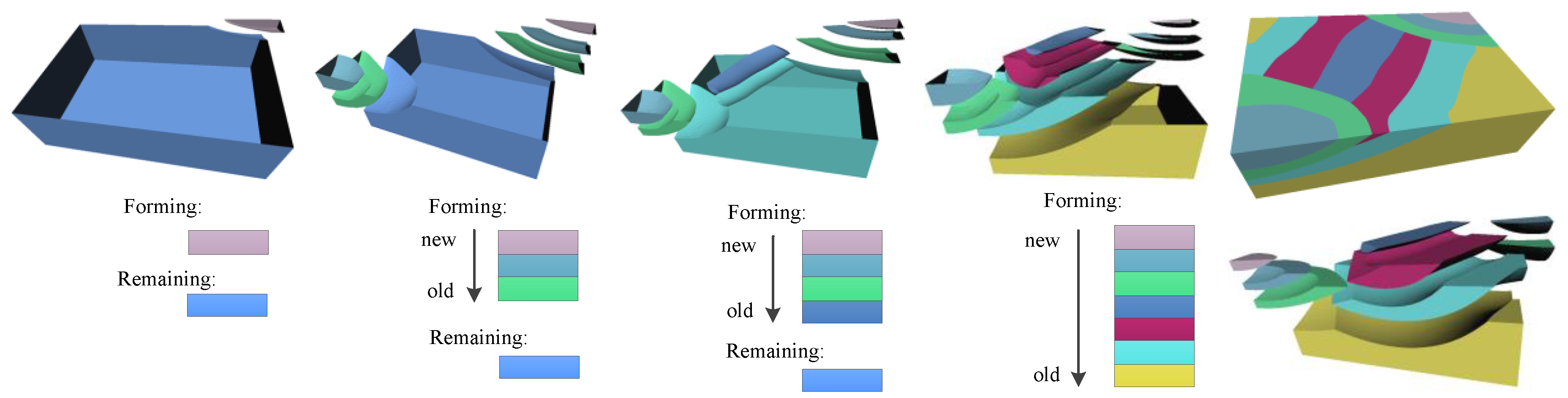
6.4. Extraction of the Geological Model

Using this implicit face-body Boolean method, the fundamental body model was divided into two models. However, after the Boolean operation, we only obtained two generated models instead of all the models. To construct all the models, an extraction method is proposed in this paper. The fundamental models belonged to different levels, and the initial model belonged to the initial level. After the first Boolean operation, we obtained two models that served as the fundamental models belonging to the next level. The fundamental models that were generated were further divided into new fundamental models. The Boolean operation was carried out until all the interfaces had divided the fundamental bodies; in other words, all the fundamental bodies became the final geological models.
When constructing the geological models using this method, it is important to assign the orders of formation of the bodies. During the formation of geological bodies, older bodies can be eroded and new bodies can be formed on these bodies through a series of geological processes, including transportation by water and deposition. Thus, old interfaces will terminate at younger interfaces when they intersect, and younger interfaces should be used in the model construction before older interfaces are used. Therefore, every time an interface divided a fundamental body, only one Boolean operation was used. The workflow is shown in Figure 5.
Although these geological models revealed the subsurface conditions of the bodies, they were not complete because the top surfaces had not been matched to each body. Using the topological relations of all of the triangles, we obtained the boundary triangles of the bodies and the insular edges of the triangles. Through point tracing, the insular edges could be connected to form closed polygons that represented the boundaries of the geological bodies. Through the corresponding boundaries, all of the top surfaces could be matched to the corresponding bodies. At this point, the workflow was complete, and the 3D geological model had been constructed. The last step in Figure 5 shows the complete models containing the top surfaces.

7. Surface Intersection

Methods for treating the intersections between the implicit surface and lines and triangles are introduced in this section. These methods were used in the body-extraction process presented in the previous section.

7.1. Surface-Segment Intersection

The HRBF function value of a point is the distance from the point to the surface. The value’s sign indicates whether the point is in the positive field or the negative field. If a segment intersects a surface, the function values of the segment’s two endpoints clearly have opposite signs. The function values were used to obtain the distances from the segment’s endpoints to the implicit surface. As shown in Figure 6a, the distance from P1 to surface P 1 H 1 ¯ is |f (P1)|, and the distance from P2 to surface P 1 H 2 ¯ is |f (P2)|. The perpendicular feet H1 and H2 of P1 and P2, respectively, and the intersection point K are approximately collinear. Under these circumstances, triangle △P1H1K is similar to triangle △P2H2K. From the characteristics of similar triangles, vertex P 1 K could be calculated as
P 1 K = L 1 L 1 + L 2 P 1 P 2
The intersection point K was calculated as P 1 + P 1 K .

7.2. Surface–Triangle Intersection

The key step in handling the intersection of interfaces with fundamental bodies was dividing the triangles by the implicit surface. The relevant method is introduced here.
If the function values of the triangle’s three points were all equal to or greater than zero, the triangle was not divided by the surface and was in the surface’s positive field. In contrast, if the function values of the triangle’s three points were all equal to or less than zero, the triangle was in the surface’s negative field.
When one segment of a triangle intersected the surface and another point’s function value was zero, the triangle was divided into two triangles with one in the surface’s positive field and one in the negative field. As shown in Figure 6b, where f(P1) = 0, f(P2) < 0 and f(P3) > 0, the triangle was divided into △P1KP3 and △P1KP2; △P1KP3 was in the positive field, and △P1KP2 was in the negative field.
When two segments of a triangle intersected the implicit surface, two intersection points occurred between the triangle and the surface. Using the two intersection points, the triangle was divided into three triangles; two were in the positive field and one was in the negative field, or one was in the positive field and two were in the negative field. As shown in Figure 6c, f(P1) > 0, f(P2) < 0, and f(P3) < 0, and the triangle was divided as △P1K1K2, △P2K1K2 and △P2P3K2. Triangle △P1K1K2 was in the positive field, and △P2K1K2 and △P2P3K2 were in the negative field.

8. Results and Analysis

A prototype system was developed based on the modeling method. The basic modeling elements, including attitudes and boundaries, were created in the system. Typical geological structures, including folds and faults, were simulated. Realistic regional geological data were tested in this system, and the corresponding 3D geological models were constructed.

8.1. Simulation of Strata

Strata are usually the simplest and most fundamental geological structures, and they are usually formed by deposition. If the deposition was not interrupted, the strata may be parallel to each other; these are called conformable strata. Correspondingly, when the deposition was interrupted by the geological process and the strata formed by the next deposition are not parallel to the previous one, the strata are referred to as unconformable. These two types of strata were simulated through the workflow in this paper. Following a sequence from new strata to old strata, each stratum was extracted from the fundamental model. The conformable strata are simulated in Figure 7a; the sections perpendicular to the strata were created. The unconformable strata are simulated in Figure 7b; the cross-sections shown on the left describe the conformable parts, and the unconformable parts are described on the right.

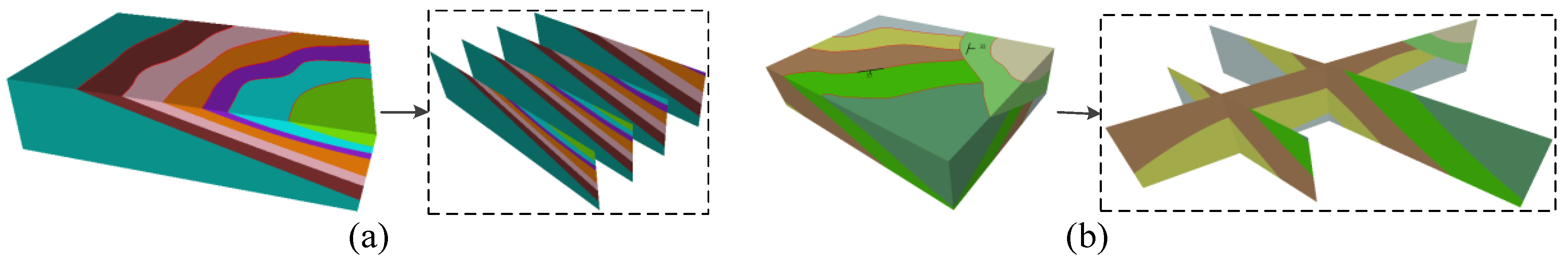
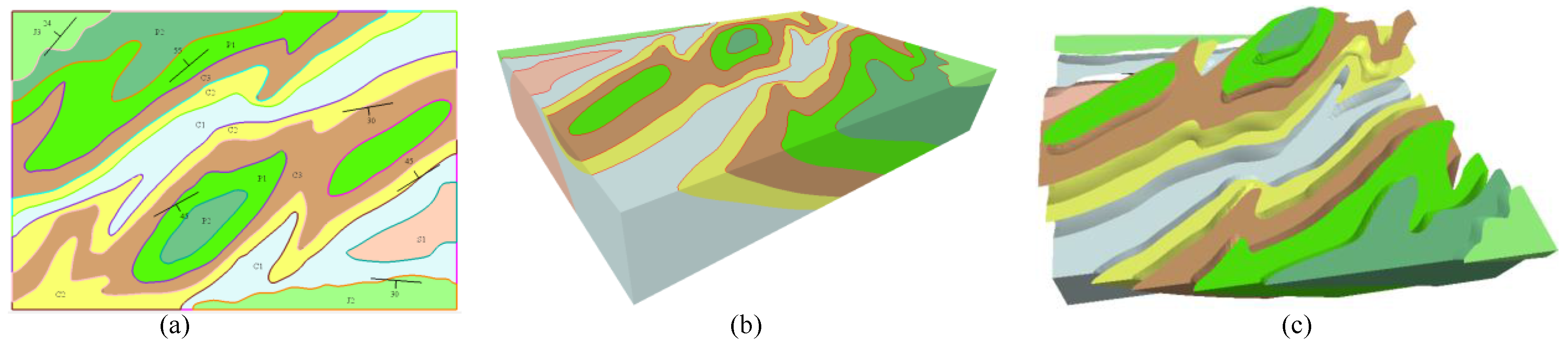
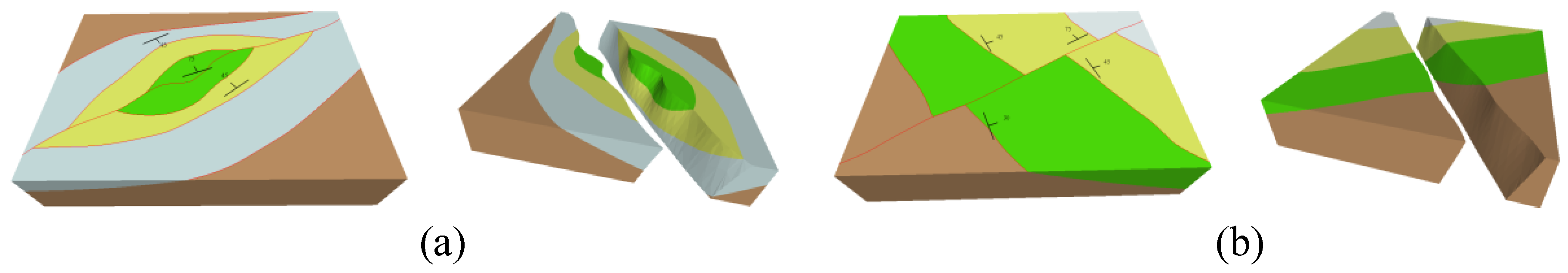
8.2. Simulation of Folds

Rock strata are usually horizontal; however, strata can be folded by geological processes, creating fundamental, significant and complex geological structures called folds. Folds can be classified into two categories, anticlines and synclines, based on the relative ages of the strata in the middle and edges of the fold. When the strata in the middle are younger, the fold is a syncline; when the strata on the edge are younger, the fold is an anticline.
Synclines are good structures for water storage and are suitable for constructing reservoirs. Thus, simulating synclines is necessary before planning this type of infrastructure. The interfaces were constructed from the HRBF surface in the subsurface by connecting the same boundaries on both limbs of the syncline. The geological bodies were constructed from the interfaces one by one from the center to the limbs. The model in Figure 8a is a simple simulation of a syncline. The structures in the middle of the models in Figure 8 are simulated synclines from geological maps.
Anticlines are good locations for oil reservoirs and are thus important structures to simulate before exploitation. Anticlines are arched structures; thus, they can act as supports in engineering applications and are suitable for tunnels. Similar to synclines, the boundaries in both limbs were drawn before constructing the model. The geological models were then constructed from the limbs to the center. The model in Figure 8b is a simple simulation of an anticline. The structures on both edges of Figure 9 are simulated anticlines from geological maps.

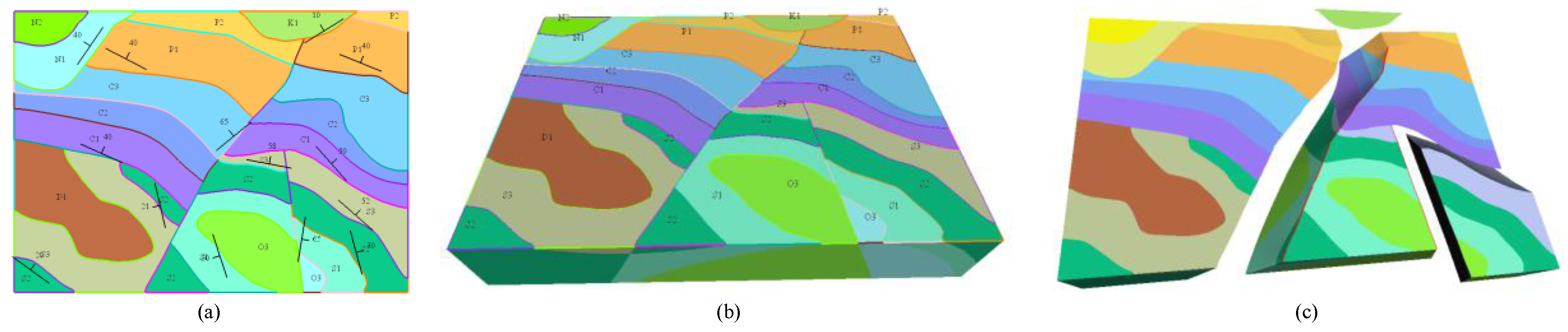
8.3. Simulation of Faults

Faults are as universal as folds and are important geological structures that form as a result of powerful geological processes that break the original structures. When simulating a fault, the fault surface should be constructed first and used as a strong modeling constraint. Under the constraints of the fault surface, the geological bodies on both sides of the fault surface were constructed. An area that contained two basic types of faults—dip-slip and strike-slip faults—was simulated.
Strike-slip faults are faults whose movements are horizontal along the fault’s strike. This type of fault is very common, and the basic conditions can be represented by the geological boundaries. The boundaries on each side of the fault surface move in opposite directions along the fault. The fault surface was constructed from the attitude of the fault, and the fundamental body was divided into two models by the fault surface. The other bodies were then extracted from these two fundamental bodies. The fault model in Figure 10b and the left fault in Figure 10 are strike-slip faults.
Dip-slip faults are faults that move vertically. Dip-slip faults are divided into two types, normal and reverse faults, based on the relative movement of the rocks and the fault surface. When the upper rocks move downward, the fault is a normal fault; when the upper rocks move upward, the fault is a reverse fault. The process of constructing dip-slip faults is nearly the same as that for strike-slip faults. The fault model in Figure 10a and the small fault in the right part of Figure 11 are normal faults because the upper rocks, which are located to the right of the fault, moved downward.

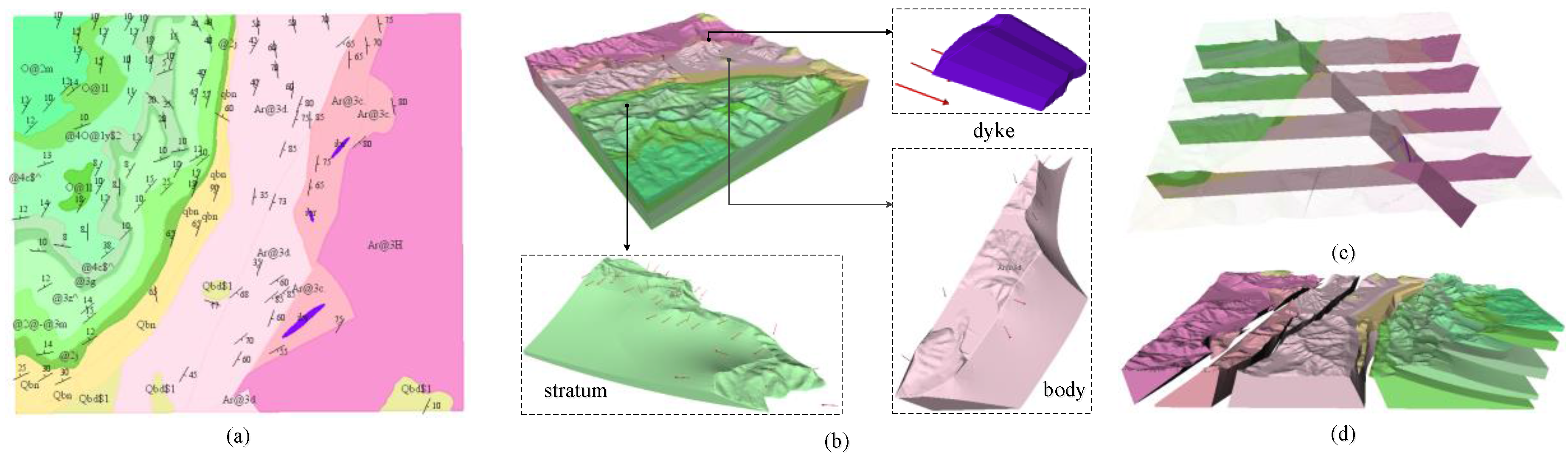
8.4. Realistic Geological Mapping

A regional geological survey region in China that contained 32 geological boundaries, 167 attitudes (Figure 12a), and 25 faults was selected for a geological modeling experiment. Three main faults are located in the middle of the study area. The strata and the rocks were divided by the left fault. The experiment was performed on a ThinkPad laptop (1.7-GHz Intel(R) Core(TM) i5-4210U, 8 GB of RAM memory, and an Intel HD graphics card).
It required five minutes to input the data into the system and generate the fundamental model of the experiment area. The order of extraction of the bodies and the modeling altitude were manually specified. The study area was relatively flat, and the average altitude of the surface was 100 m. We set the modeling altitude as –1000 m, which meant that the maximum depth of the models was approximately 1100 m. The system required 4 min 21 s to construct the entire model, including 1 min 46 s to calculate the top surface and 2 min 35 s to generate the subsurface model. The model contained 199,909 triangles. The system provided rapid, accurate and automatic simulations of a wide range of regional geological bodies.
Cross-sections were used to analyze the modeling results. The geological conditions of the area were displayed in five cross-sections. The strata on the left, the rocks on the right and the dividing line between them are shown in Figure 12c. The crushed zone, which was produced by faulting at the intersection between the strata and the rocks, is also shown on the cross-sections.
The strata are shown clearly in the exploded view of the geological model (Figure 12d). The modeling results showed that the proposed method is suitable for generating geological models, especially strata and body models (Figure 12b). The spatial extent and continuity of the strata were accurately expressed by the HRBF surface. The topological consistency of the models was also guaranteed by the Boolean operation. In general, the method constructed the 3D regional geological model automatically and rapidly.
It should be noted that the models were merely constrained by the attitudes. To create more accurate models, more constrained data, such as drill-holes, are required. However, drill-hole data were very scarce in the regional geological survey. For the purpose of constraining the models by drill-holes, some virtual drill-holes (Figure 13a) were constructed in this paper. The geological interfaces were constrained by the drill-hole points and the model shown in figure 13b extending vertically was modified. The models in the area constrained by the drill-holes were constructed through the implicit surface method (Figure 13c).
Modeling efficiency is a very important index to evaluate the modeling algorithm. There are mainly three time-consuming parts of our modeling workflow: the equation solving part, the plumb scanning implicit surface reconstruction part and the terrain surface construction part. Furthermore, the first two parts are separated from the third part. Meanwhile, the time of equation solving part is decided by the points of the boundaries, which are decided by the geological maps. Thus, we conduct efficiency testing experiments of the plumbing scanning implicit surface construction part and the terrain surface construction part.
To the terrain surface construction part, we carried out the efficiency test of the through changing the DEM points. With the variation of the terrain points, the time to construct the terrain surface was recorded and the time to point count figure was drawn. It is clear in Figure 14 that the modeling time was linear dependent to the point count, which meant the algorithm was relatively stable when the DEM points were less than 200,000 (Table 1).
To the plumb scanning implicit surface construction, we use different mesh grid lengths to test the efficiency of the work flow. The relation between the consuming time and the grid length is shown in Table 2. It shows that when the grid length was more than 300 meters, the extracting time was nearly invariable. It indicated that when the grid length was more than 300 meters, the equation solving part was the main consumer of the modeling time.
The time and reciprocal of the quadratic of the grid length was drawn in the Figure 15, which showed that the time was proportional to the reciprocal of the quadratic of the grid length. When the grid length increases, the point counts will increase not only in the X direction, but also in the Y direction. The direct ratio relation shows that the algorithm is stable (Table 2).

9. Conclusions and Future Work

A method for constructing 3D geological models was proposed in this paper. The geological interfaces were constructed from the geological boundaries and were constrained by the attitudes. A fundamental body was constructed based on the map boundary. Using the HRBF implicit surface intersection method, the fundamental body was divided into geological bodies by the geological interfaces. The 3D geological model was completed by adding the top surfaces, which were constructed from the geological boundaries and the DEM. A prototype system was developed to simulate typical structures with the system. An experiment was performed using realistic data, and the corresponding 3D geological models were developed rapidly and accurately.
A completely new HRBF surface-body Boolean method was designed to extract the geological models from the fundamental body. In contrast to the CSG Boolean method, this method only used the function of the surface instead of a triangular mesh model. The triangles were divided only by the function values of the three vertexes. The implicit surface was sampled using plumb scanning lines, and the interface was constructed by coupling the sampling points and its boundary polygon. This method ensured that the interfaces pass through the boundaries, which forced the subsurface body models to correspond to the top surfaces. The construction method that used scanning lines was much more rapid than methods that use marching cubes or marching tetrahedrons. Thus, the geological models could be constructed more rapidly and accurately.
Because the interfaces were constructed through the boundaries constrained by attitudes, this method cannot simulate multilayered geological bodies or bodies that have large spatial variations such as plunging folds. In future work, we plan to use drill-hole data, cross-section data and some soft data, including seismic data, to further constrain the subsurface conditions. In addition, multilayered structures, such as salt domes, will be simulated.

Acknowledgments

This research is jointly supported by the Liaoning Province Natural Science Foundation (2015020581), the Fundamental Research Funds for the Central Universities (N140104002) and China Geological Survey Projects (1212011120436, 12120115073201).

Author Contributions

Jiateng Guo and Lixin Wu conceived and designed the experiments; Wenhui Zhou and Jizhou Jiang performed the experiments; Chaoling Li collected the realistic modeling data and checked the models; Wenhui Zhou and Jizhou Jiang wrote the modeling codes; Jiateng Guo and Wenhui Zhou wrote the paper.

Conflicts of Interest

The authors declare no conflict of interest.

References

  1. Jacobsen, L.J.; Glynn, P.D.; Phelps, G.A.; Orndorff, R.C.; Bawden, G.W.; Grauch, V.J.S. US Geological Survey: A Synopsis of Three-Dimensional Modeling; US Geological Survey: Reston, VA, USA, 2011.
  2. Mallet, J.L. GOCAD: A Computer Aided Design Program for Geological Applications, Three-Dimensional Modeling with Geoscientific Information Systems; Springer: Houten, The Netherlands, 1992. [Google Scholar]
  3. Kessler, H.; Mathers, S.; Sobisch, H.G. The capture and dissemination of integrated 3D geospatial knowledge at the British Geological Survey using GSI3D software and methodology. Comput. Geosci. 2009, 35, 1311–1321. [Google Scholar] [CrossRef] [Green Version]
  4. Scheck-Wenderoth, M.; Lamarche, J. Crustal memory and basin evolution in the Central European Basin System—New insights from a 3D structural model. Tectonophysics 2005, 397, 143–165. [Google Scholar] [CrossRef]
  5. Alaei, B. Seismic Modeling of Complex Geological Structures; INTECH Open Access Publisher: Rijeka, Croatia, 2012. [Google Scholar]
  6. Raiber, M.; White, P.A.; Daughney, C.J.; Tschritter, C.; Davidson, P.; Bainbridge, S.E. Three-dimensional geological modelling and multivariate statistical analysis of water chemistry data to analyse and visualise aquifer structure and groundwater composition in the Wairau Plain, Marlborough District, New Zealand. J. Hydrol. 2012, 436, 13–34. [Google Scholar] [CrossRef]
  7. Borghi, A.; Renard, P.; Courrioux, G. Generation of 3D spatially variable anisotropy for groundwater flow simulations. Groundwater 2015. [Google Scholar] [CrossRef] [PubMed]
  8. McGaughey, J.; Milkereit, B. Geological models, rock properties, and the 3D inversion of geophysical data. In Proceedings of the Exploration 07: Fifth Decennial International Conference on Mineral Exploration, Toronto, ON, Canada, 9–12 September 2007; pp. 473–483.
  9. Calcagno, P. 3D GeoModelling for a democratic geothermal interpretation. In Proceedings of the 2015 World Geothermal Congress, Melbourne, Vic, Australia, 19–25 April 2015.
  10. Jia-teng, G.; Li-xin, W.; Yi-zhou, Y.; Wen-hui, Z. Three-Dimensional Modeling and Visualization Information Management of Geotechnical Engineering Investigation Sites. J. Northeast. Univer. (Nat. Sci.) 2014, 1, 122–125. [Google Scholar]
  11. Jia-teng, G.; Rong-bing, Z.; Li-xin, W.; Yi-zhou, Y. An automatic method for generating curvilinear geological section with stratal pinch-out. In Proceedings of the 2011 IEEE International Geoscience and Remote Sensing Symposium (IGARSS), Vancouver, BC, Canada, 24–29 July 2011.
  12. Jia-teng, G.; Yi-zhou, Y.; Li-xin, W.; Rong-bing, Z. A novel method for modeling complex 3D geological body with stratal pinch-out. In Proceedings of the 2011 IEEE International Geoscience and Remote Sensing Symposium (IGARSS), Vancouver, BC, Canada, 24–29 July 2011.
  13. Hong-bin, M.; Jia-teng, G. Study on Facial-Volumetric Mixed 3D Geological Modeling Based on Sections. J. Metal Mine. 2007, 7, 50–52. [Google Scholar]
  14. Ming, J.; Pan, M.; Qu, H.; Ge, Z. GSIS: A 3D geological multi-body modeling system from netty cross-sections with topology. Comput. Geosci. 2010, 36, 756–767. [Google Scholar] [CrossRef]
  15. Thorleifson, L.H.; Berg, R.C.; Russell, H.A.J. Geological mapping goes 3-D in response to societal needs. GSA Today 2010, 20, 27–29. [Google Scholar] [CrossRef]
  16. Turner, A.K. Challenges and trends for geological modelling and visualisation. Bull. Eng. Geol. Environ. 2006, 65, 109–127. [Google Scholar] [CrossRef]
  17. Amorim, R.; Brazil, E.V.; Samavati, F.; Sousa, M.C. 3D geological modeling using sketches and annotations from geologic maps. In Proceedings of the 4th Joint Symposium on Computational Aesthetics, Non-Photorealistic Animation and Rendering, and Sketch-Based Interfaces and Modeling, New York, NY, USA, 8–10 August 2014; pp. 17–25.
  18. Breen, D.E.; Mauch, S.; Whitaker, R.T. 3D scan conversion of CSG models into distance volumes. In Proceedings of the 1998 IEEE Symposium on Volume Visualization, New York, NY, USA, 19–20 October 1998.
  19. Tseng, Y.H.; Wang, S. Semiautomated building extraction based on CSG model-image fitting. Photogramm. Eng. Remote Sens. 2003, 69, 171–180. [Google Scholar] [CrossRef]
  20. Sun, T.L.; Su, C.J.; Mayer, R.J.; Wysk, R.A. Shape similarity assessment of mechanical parts based on solid models. In Proceedings of the 1995 ASME Design Engineering Technical Conference, Boston, MA, USA, 17–20 September 1995.
  21. You, L.H.; Zhang, J.J.; Comninos, P. Generating blending surfaces with a pseudo-Levy series solution to fourth order partial differential equations. Computing 2003, 71, 353–373. [Google Scholar] [CrossRef]
  22. De Araújo, B.R.; Jorge, J.A.P. Curvature dependent polygonization of implicit surfaces. In Proceedings of the 17th Brazilian Symposium on Computer Graphics and Image, Curitiba, PR, Brazil, 17–20 October 2004.
  23. Macedo, I.; Gois, J.P.; Velho, L. Hermite radial basis functions implicits. Comput. Graphics Forum 2011, 30, 27–42. [Google Scholar] [CrossRef]
  24. Hillier, M.; de Kemp, E.; Schetselaar, E. 3D form line construction by structural field interpolation (SFI) of geologic strike and dip observations. J. Struct. Geol. 2013, 51, 167–179. [Google Scholar] [CrossRef]
  25. Hillier, M.J.; Schetselaar, E.M.; de Kemp, E.A.; Perron, G. Three-dimensional modelling of geological surfaces using generalized interpolation with radial basis functions. Math. Geosci. 2014, 46, 931–953. [Google Scholar] [CrossRef]
  26. Natali, M.; Klausen, T.G.; Patel, D. Sketch-based modelling and visualization of geological deposition. Comput. Geosci. 2014, 67, 40–48. [Google Scholar] [CrossRef]
  27. Knight, R.H.; Lane, R.G.; Ross, H.J.; Abraham, A.P.G.; Cowan, J. Implicit ore delineation. In Proceedings of the Fifth Decennial International Conference on Mineral Exploration, Toronto, ON, Canada, 9–12 September 2007; pp. 1165–1169.
  28. Cowan, E.J.; Beatson, R.K.; Fright, W.R.; McLennan, T.J.; Mitchell, T.J. Rapid geological modelling. Appl. Struct. Geol. Min. Explor. Min. 2002, 36, 39–41. [Google Scholar]
  29. What is Micromine? Available online: http://www.micromine.com/products-downloads/micromine (accessed on 20 December 2015).
  30. Vulcan. Available online: http://www.maptek.com/products/vulcan/ (accessed on 20 December 2015).
  31. Alcaraz, S.; Lane, R.; Spragg, K.; Milicich, S.; Sepulveda, F.; Bignall, G. 3D geological modelling using new Leapfrog Geothermal software. In Proceedings of the 36th Workshop on Geothermal Reservoir Engineering, Stanford, CA, USA, 31 January–2 February 2011.
  32. Calcagno, P.; Chilès, J.P.; Courrioux, G.; Guillen, A. Geological modelling from field data and geological knowledge: Part I. Modelling method coupling 3D potential-field interpolation and geological rules. Phys. Earth Planet. Inter. 2008, 171, 147–157. [Google Scholar] [CrossRef]
  33. Bistacchi, A.; Massironi, M.; Dal Piaz, G.V.; Dal Piza, G.; Monopoli, B.; Schiavo, A.; Toffolon, G. 3D fold and fault reconstruction with an uncertainty model: An example from an Alpine tunnel case study. Comput. Geosci. 2008, 34, 351–372. [Google Scholar] [CrossRef]
  34. Suzuki, S.; Caumon, G.; Caers, J. Dynamic data integration for structural modeling: Model screening approach using a distance-based model parameterization. Comput. Geosci. 2008, 12, 105–119. [Google Scholar] [CrossRef]
  35. Wellmann, J.F.; Horowitz, F.G.; Schill, E.; Regenauer-Lieb, K. Towards incorporating uncertainty of structural data in 3D geological inversion. Tectonophysics 2010, 490, 141–151. [Google Scholar] [CrossRef]
  36. He, X.; Koch, J.; Sonnenborg, T.O.; Jørgensen, F.; Schamper, C.; Christian Refsgaard, J. Transition probability-based stochastic geological modeling using airborne geophysical data and borehole data. Water Resour. Res. 2014, 50, 3147–3169. [Google Scholar] [CrossRef]
  37. Feito, F.R.; Ogáyar, C.J.; Segura, R.J.; Rivero, M.L. Fast and accurate evaluation of regularized Boolean operations on triangulated solids. Comput. Aided Des. 2013, 45, 705–716. [Google Scholar] [CrossRef]
  38. Zlatanova, S.; Rahman, A.; Shi, W. Topological models and frameworks for 3D spatial objects. Comput. Geosci. 2004, 30, 419–428. [Google Scholar] [CrossRef] [Green Version]
  39. Hong-bin, M.; Jia-teng, G.; Qun, H.E.; Xin-rui, L. Study on Delaunay triangulation algorithm for polygon with inside islets. J. Northeast. Univer. (Nat. Sci.) 2009, 5, 733–736. [Google Scholar]
  40. Jia-teng, G.; Li-xin, W.; Yi-zhou, Y.; Rong-bing, Z. Towards a seamless integration for spatial objects and topography. In Proceedings of the 2012 IEEE International Conference on Geoinformatics (GEOINFORMATICS), Hong Kong, China, 15–17 June 2012.
  41. Hong-bin, M.; Jia-teng, G. Cut-and-sew algorithm: A new multi-contour reconstruction algorithm. J. Northeast. Univer. (Nat. Sci.) 2007, 1, 111–114. [Google Scholar]
Figure 1. Modeling workflow.
Ijgi 05 00017 g001
Figure 2. Top surfaces.
Ijgi 05 00017 g002
Figure 3. Fundamental body.
Ijgi 05 00017 g003
Figure 4. Geological interface created by the geological boundary through HRBF and the fundamental body divided by the geological interface.
Ijgi 05 00017 g004
Figure 5. Sequential extraction of geological models from the fundamental body from new to old.
Ijgi 05 00017 g005
Figure 6. Surface-related intersections. (a) The segment intersects the HRBF surface; (b) a triangle with one point on the surface intersects the surface; and (c) a triangle with no points on the surface intersects the surface.
Ijgi 05 00017 g006
Figure 7. Simulated strata: (a) conformable strata and sections perpendicular to the strata and (b) unconformable strata and cross-sections describing the conformable and unconformable parts.
Ijgi 05 00017 g007
Figure 8. Simulated folds: (a) syncline and (b) anticline.
Ijgi 05 00017 g008
Figure 9. Fold models from a geological map: (a) the 2D geological map with attitudes that describe the geological conditions; (b) 3D geological model; and (c) exploded view of the model.
Ijgi 05 00017 g009
Figure 10. Fault models: (a) normal dip-slip fault models; and (b) strike-slip fault models.
Ijgi 05 00017 g010
Figure 11. Fault models from a geological map: (a) 2D geological map containing two faults; (b) 3D geological model; and (c) exploded view of the geological model divided by the faults.
Ijgi 05 00017 g011
Figure 12. Realistic geological model: (a) 2D geological map of the study area; (b) 3D geological model, the three main parts of the model and the constraining attitudes’ displayed as arrows; (c) cross-sections of the geological model; and (d) exploded view of the models.
Ijgi 05 00017 g012
Figure 13. Geological models constrained by Drill-hole data: (a) virtual drill-hole data constructed in the area containing stratum; (b) the geological model that extended vertically was modified by the drill-holes; and (c) the stratum model constrained by the drill-holes.
Ijgi 05 00017 g013
Figure 14. Terrain surface modeling time with respect to the DEM point count. The modeling time was linear dependent to the point count.
Ijgi 05 00017 g014
Figure 15. Plumb scanning implicit construction time with respect to the reciprocal of the quadratic of the grid length. The modeling time was nearly proportional to the reciprocal of the quadratic of the grid length.
Ijgi 05 00017 g015
Table 1. Time consuming experiment with respect to different DEM point count.
Point CountTime/s
50008
10,00015
20,00030
50,00081
100,000147
200,000293
Table 2. Time consuming of implicit surface construction with respect to grid length.
Grid Length/mTime/s
50698
70324
80256
90215
100172
20087
30064
40061
50060

