Article

A GIS Study of the Influences of Warm Ocean Eddies on the Intensity Variations of Tropical Cyclones in the South China Sea

1
School of Resource and Environmental Sciences, Wuhan University, 430079 Wuhan, China
2
State Key Laboratory of Resources and Environmental Information System, Institute of Geographic Science and Natural Resources Research, Chinese Academy of Sciences, 100101 Beijing, China
3
Key Laboratory for Geo-Environmental Monitoring of Coastal Zone of the National Administration of Surveying, Mapping and GeoInformation & Shenzhen Key Laboratory of Spatial Smart Sensing and Services & College of Life Sciences and Oceanography, Shenzhen University, 518060 Shenzhen, China
*
Authors to whom correspondence should be addressed.
ISPRS Int. J. Geo-Inf. 2016, 5(10), 169; https://doi.org/10.3390/ijgi5100169
Submission received: 23 June 2016 / Revised: 14 September 2016 / Accepted: 19 September 2016 / Published: 23 September 2016

Abstract

:
This study presented the spatial distribution patterns of tropical cyclones (TCs) in the South China Sea (SCS) and discussed the possible influences of average sea surface temperature (SST) and the size of warm ocean eddies on changes in the intensity of TCs passing over them. Between 1993 and 2013, the SCS has experienced 233 TCs, of which 134 have interacted with warm ocean eddies. The results of fuzzy c-means (FCM) clustering showed that these TCs are mainly located in the northern portion of the SCS. After interacting with warm ocean eddies, TCs may intensify, remain at the same intensity, or weaken. For intensifying TCs, the enhancements range from 0 to 3 m/s only; however, this level of TC intensity enhancement is statistically significant at p<0.05. Further statistical analyses show that warm ocean eddies with a higher-than-average SST and a larger ratio between the size of the warm ocean eddies and the radius of the TC maximum wind may help intensify passing TCs.

1. Introduction

Tropical cyclones (TCs) are a common natural phenomenon that usually cause devastating disasters and, thus, significantly affect human social and economic activities. After a TC makes landfall, it usually causes significant loss of life, damage to city infrastructure, and ecosystem destruction. For example, when Katrina swept across the northern Gulf Coast of the United States, it caused about 1500 deaths and a total damage of about $81 billion [1]. In the Western Pacific Ocean, the super typhoon Maemi, in 2003, was the most destructive TC. The storm surge produced by Maemi claimed approximately 130 lives and caused $5 billion in property damage in Korea [2]. The TC Nargis was one of the most devastating natural disasters in the North Indian Ocean in recent years; bringing approximately 600 mm of total rainfall and a storm surge 3–4 m high, flooding the low-lying and densely populated Irrawaddy River delta. The deaths and missing persons toll from Nargis exceeded 130,000, and the economic losses were more than $10 billion [3,4].
Predicting the tracks of TC as well as their intensity changes along these tracks is of great value to society. A few systems have been developed and utilized successfully to track TCs, such as the Global Forecast System (GFS) of the National Oceanic and Atmospheric Administration (NOAA), the NOAA/Geophysical Fluid Dynamics Laboratory’s (GFDL) regional hurricane forecasting system, the U.S. Navy Operational Global Atmospheric Prediction System (NOGAPS), the European Centre for Medium-Range Weather Forecasts (ECMWF) model, and the Met Office model (UKMET) [5]. However, in the past decade, the ability to forecast TC intensity changes has continuously lagged far behind the ability to forecast their paths [5,6]—mainly because TC intensity changes are affected by a multitude of factors [7,8,9,10,11]. One significant factor is the sea surface temperature in the regions over which a TC passes.
Previous studies have reported sudden and unexpected intensification of TCs passing over warm ocean areas such as ocean currents and warm ocean eddies [8,12,13,14,15,16]. For example, in 1995, Hurricane Opal strengthened from 965 to 916 hPa within 14 h after encountering a warm ocean eddy in the Gulf of Mexico. The intensification process can be attributed to both the upper-ocean thermal structure and to lower atmospheric anomalies. However, the former tends to play a more important role than the latter in its effect on TC intensity variations [17,18]. Warm ocean eddies possibly serve as a heat reservoir to supply heat energy that intensifies passing TCs. They may also act as an effective insulator between TCs and the deeper cold ocean water [19,20]. Warm ocean eddies are characterized by a distinctly deep and thick 26 °C isothermal layer, whose characteristics could be used to measure hurricane heat potential [21]. When a TC encounters a warm ocean eddy, the upper-ocean mixed layer of the warm ocean eddy tends to prevent the cold water beneath from upwelling; consequently, the sea surface temperature does not drop as significantly as in areas lacking warm ocean eddies. Such an effect has been identified from both observation data and from the results of numerical experiment [12,13,18,19,22,23,24,25,26,27,28,29]. For example, as Hurricane Opal swept across the Gulf of Mexico, post-storm sea surface temperatures (SST) fell by approximately 0.5 °C and 2 °C in the areas with and without warm ocean eddies, respectively.
Ocean eddies, which are ubiquitous ocean phenomena [30,31], play an important role in transporting and exchanging both physical and chemical constituents (i.e., heat, momentum, mass, chlorophyll) within oceans [32,33,34]. Both warm and cold ocean eddies may modify the upper-ocean mixed layer. These typically affect TC intensity variations in totally opposite ways: warm and cold eddies tend to intensify and weaken passing TCs, respectively [18,35]. In this study, we focused primarily on the relationship between warm ocean eddies and TCs.
Numerical modelling results provide important insights about the influences of warm ocean eddies on TC intensity changes [12,13,19,22,23,24]. Currently, the interaction processes between warm ocean eddies and TCs can be simulated using hurricane-ocean coupled models such as the Coupled Hurricane Intensity Prediction System (CHIPS) model [19], the axisymmetric hurricane model and the four-layer ocean model [22]. These modelling results can be used to evaluate the effects of different factors on TC intensity and reveal the physical mechanisms that drive the interactions between these two phenomena. However, the modelling results tend to vary on a case-by-case basis; therefore, they cannot be used to investigate the interactions between warm ocean eddies and TCs over a broad area.
Vianna et al. [29] conducted a case study to evaluate how warm ocean eddies affected Hurricane Catarina using Argo data and high-resolution satellite-derived data including ocean surface wind, sea surface height and SST. They concluded that warm ocean eddies intensified Hurricane Catarina, although, unlike numerical modeling, this type of case study is unable to evaluate how individual factors affect TC intensity variations.
Oropeza et al. [36] used the National Hurricane Center’s archived best-track data from 1993 to 2009 to study how warm ocean eddies rapidly strengthened TCs in the northeastern Tropical Pacific. The statistical analysis results showed that warm ocean eddies are favorable to strengthening TCs. They concluded that the local heat exchange between the ocean and the TC increased when a TC swept over a region with warm ocean eddies. They also estimated the change in ocean heat content in response to warm ocean eddies using an algorithm developed by Goni et al. [37] and Shay et al. [12]. However, this study suffers from a few limitations. First, as the authors noted, it is not appropriate to simply use the heat content of the water to identify warm ocean eddies. Second, defining the extent of a warm ocean eddy based on high water heat content and positive sea surface anomalies is not a scientifically strict approach. Thus, it would be of great value, as we did in this study, to examine the interactions between TCs and warm ocean eddies using more rigorous methods based on more clearly defined criteria [38].
Geographic information systems (GIS) technology has superior spatial data management, analysis, and presentation capabilities [39] and has been widely used in urban transport planning [40,41], environmental studies [42], disease spreading models [43], and disaster response fields [44]. GIS has also been employed in meteorology to forecast typhoon tracks [45]. Both TC tracks and warm ocean eddies have spatial characteristics and thus can be translated into spatial data and then examined in GIS to reveal the spatial distribution patterns of the interactions between warm ocean eddies and TCs over a broad area.
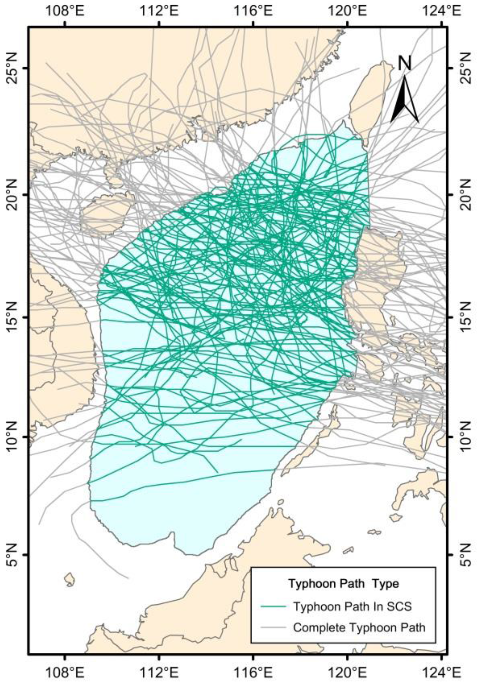
This study uses a long-duration time series (1993–2013) dataset of warm ocean eddies and TCs to examine the interaction between these two types of phenomena. In addition to evaluating the effects of warm ocean eddies on TC intensity changes, and further to validate results from previous studies; however, over a much broader area (i.e., the South China Sea (SCS)).

2. Data and Methods

2.1. Study Area

The SCS is the largest semi-enclosed marginal sea in the Northwest Pacific. It is one of the most important areas frequently affected by TCs [46,47]. Mesoscale eddies are ubiquitous across the SCS and play an important role in regional energy exchange and material transport [33,48,49,50,51]. Previous studies have shown that warm ocean eddies also affect TC intensity changes in the SCS [52]; however, it is still not clear how warm ocean eddies interact with TCs and whether the interactions vary across the SCS. A better understanding of such interactions is significant in TC forecasting, which is vital to the people living in areas that are vulnerable to TCs.

2.2. Altimetry, TC, and Sea Surface Temperature Data

We used three main datasets in this study, including the TC dataset, sea surface temperature (SST) dataset, and sea level anomaly maps. The TC dataset provides information about the optimum TC tracks and variations in the relative intensity of TCs. The SST data were used to derive the surface temperature of warm ocean eddies, which were extracted from the 1993–2013 sea level anomaly maps.
The sea level anomaly maps are a merged product of several available satellite missions (HY-2A, Saral/AltiKa, Cryosat-2, Jason-1, Jason-2, T/P, Envisat, GFO, ERS1/2 and Geosat data), with a spatial resolution of 1/4° × 1/4° and a daily temporal resolution. The 1993–2013 sea level anomaly maps were extracted and downloaded from the Archiving, Validation and Interpretation of Satellite Oceanographic Data (AVIOS) web site (http://www.aviso.altimetry.fr/en/home.html). The sea level anomaly data of shelf areas with water depths less than 200 m were masked out and not used in this study due to precision issues [53,54].
The 1993–2013 TC data were obtained from the Shanghai Typhoon Institute of the China Meteorological Administration (http://www.typhoon.gov.cn). Previous studies [55,56] have shown that the TC dataset is reliable due to the deployment of a dense observation network since the 1950s. In this study, we used the TC “best track data”, which includes the central location, minimum central pressure, and 2-min maximum central sustained wind speeds of TCs at 6-h intervals along each TC track. The radii of the maximum winds of TCs, which have been available since 2003, were obtained from the Joint Typhoon Warning Center (JTWC) (http://www.usno.navy.mil/JTWC/). The TCs were classified into six broad categories based on their maximum sustained surface wind speed and maximum wind scale according to the National Standard of China (GB/T 19201–2006) (Table 1).
The SST data were obtained from NOAA/OAR/ESRL PSD (http://www.esrl.noaa.gov/psd/data/gridded/data.noaa.oisst.v2.highres.html). This dataset consists of the daily Optimum Interpolation SST data (OISST, V2), which were derived from a High Resolution SST Dataset released by NOAA. The SST data were produced by combining global observations from multiple platforms (satellites, ships, and buoys) and the dataset has a spatial resolution of 1/4° × 1/4°.

2.3. Methodology

2.3.1. Eddy Identification

The Okubo-Weiss [57,58] and the sea surface height-based methods [30] are the most widely used methods for automatic eddy identification. The Okubo-Weiss method is mainly based on physical parameters. The physical parameter, W, for detecting ocean eddies from sea level anomaly is defined as follows:
W = Sn 2 + Ss 2 ω 2 ,
where Sn is the shear deformation, Ss is the strain deformation, and ω is the vertical component of vorticity. Usually, sea surfaces with a W less than −0.2σww is the spatial standard deviation of W) are identified as ocean eddies. In contrast, the sea surface height-based method requires no threshold for eddy identification. The method defines an area as an eddy if there is at least one local extreme sea surface height value inside an eddy-dominant region. However, these two methods both suffer their own drawbacks and the identification results are significantly affected by noise either induced in the process of calculating the physical parameters or the sea surface height anomaly field.
In this study, eddies were identified using a hybrid detection method [38]. This method essentially combined the ideas from the two previously mentioned methods. In other words, an eddy should have a core area with a circular or spiral flow pattern and a local extreme sea surface height value inside the core area. The hybrid method first identifies the “core area” of an eddy according to the W values. Then, the local extreme value of sea surface height anomaly within the core area is then identified as the center of the eddy. Finally, the outermost sea surface height anomaly isoline (an interval of 0.5 cm) that fully encloses the core area of the eddy is identified as the eddy’s boundary. A previous study [38] showed that the hybrid method is very successful in identifying ocean eddies in the SCS.

2.3.2. Identification of the Interacting TCs and Warm Ocean Eddies

We used GIS to select all TCs and ocean eddies that mutually interacted during the period from 1993 to 2013 in the SCS based on the spatial-temporal matching scheme shown in Figure 1. The TC tracks and ocean eddies were all mapped in GIS. TC tracks are selected when, at any time during their lifespans, any of their track points is located within the sea surface of an identified warm ocean eddy. At the same time, we also extracted all warm ocean eddies that contain at least one TC track point. Hereafter, the TC and warm ocean eddies specifically refer to those extracted using this matching scheme, unless otherwise specified.
Figure 2 shows how track points were generated from the original TC track data. Originally, the TC best tracks were recorded every six hours; however, that interval is too coarse to capture the situations when a TC just touches and then leaves a warm ocean eddy. Therefore, we linearly resampled the best TC tracks using a one-hour interval. We then calculated the variations in TC intensity, i.e., the difference between the maximum wind speed at the points when a TC first touches and first leaves an eddy.

2.3.3. TC Pattern Analysis

We used a fuzzy c-means clustering (FCM) algorithm [59], which has been used previously to cluster typhoon tracks [60,61], to examine the spatial pattern of the TCs. Unlike hard clustering methods, the FCM uses a membership degree to measure the probability for a data object to be placed in a cluster based on the minimum value of the c-means function:
J m = i = 1 C k = 1 N μ i k m x k c i 2 ,
where
μ i k = [ j = 1 C ( x k c i / x k c j ) 2 / ( m     1 ) ] 1 ,
and
c i = k = 1 N μ i k m x k k = 1 N μ i k m ,
The membership coefficient, μ i k , is a measure of the membership degree of the k-th data object to cluster i, where μ i k 0 and i = 1 C μ i k = 1 ; C is the number of clusters, and N is the number of data objects, and m is a fuzziness coefficient that is greater than 1 that controls the overlap degree among clusters. When m is set to a small value, data objects that are closer to the cluster center will be assigned a greater weight. Just as in other FCM studies [60,61], in this study, m is also set to 2.
The FCM also requires a threshold distance to be defined that depends on a certain number of clusters in the dataset. The average similarity index is used to define a general cluster separation measure function, R(Si, Sj, Mij), which measures the average similarity between each cluster and its most similar cluster [62]. The cluster separation function is calculated as follows:
R ¯ = 1 N i = 1   N R i ,
where   R i maximum   of   R i j , i j , and N is the number of clusters. Here,
R i j S i + S j M i j ,
where R ¯ is the average similarity measure for the entire system. The optimum clustering result is obtained when R ¯ reaches its minimum value. Si and Sj are dispersion measures for cluster i and j, respectively. Mij is the distance between the centers of clusters i and j, respectively. The similarity index is then defined by:
S i = { 1 T i j = 1 T i | X j A i | q } 1 q ,
where Ti is the number of vectors in cluster i, Xj is the member of cluster i, and Ai is the center of cluster i. Finally,
M i j = { k = 1 N | α k i α k j | p } 1 p ,
where αki is the kth component of the vector αi, which is the centroid of cluster i. The parameter p is 2 and q is 1.

2.3.4. Grid-Based Maximum Wind Speed Variation

We also calculated a long-term average of the variations in maximum wind speed for each 1/4° × 1/4° sea-level anomaly map cell. In this study, a variation in maximum wind speed is defined as the difference of the maximum wind speed between any two adjacent points along a specific TC track. We then summarized the long-term average of the variations in maximum wind speed for all TC tracks passing over the SCS from 1949 to 2013 within each cell, regardless of whether a warm ocean eddy was present within the cell when the TC passed over. We then compared the intensity changes of TCs that interacted with warm ocean eddies against the long-term average of the grid-based maximum wind speed variation to examine the possible influence of warm ocean eddies on TC intensity changes.

3. Results

3.1. General Characteristics of TC Tracks

During the period from 1993 to 2013, 233 TCs passed over the SCS. Of these, 134 interacted with warm ocean eddies (Figure 3). Visually, the TC tracks are mainly clustered in the northern SCS; fewer are found passing across the central SCS, and even fewer pass across the southern SCS. We then grouped the TC tracks into clusters to better illustrate their spatial distribution pattern quantitatively. The optimum number of clusters that the TC tracks were grouped into was selected based on the average similarity index, which was calculated after 1000 iterations of the clustering algorithm. Figure 4 shows the variations in the average similarity index in response to the different numbers of clusters into which the TC tracks were grouped.
As shown in Figure 4, grouping the TC tracks into two or three clusters shows the lowest average similarity index (1.08 and 1.30, respectively). However, these two clustering schemes show only a very general western movement trend (clusters ①, ②, and ③ in Figure 5) of the TCs and only at the cost of losing local patterns. Grouping the TC tracks into seven or eight clusters shows more local clusters (⑦ and ⑧ in Figure 5). However, only 8.21% of the TC tracks were grouped into these two clusters, respectively. As a result, we grouped the TC tracks into six clusters to ensure a low average similarity index and also maintain a membership rate of no less than 10%.
Figure 6 shows the six clusters of TC tracks atop the warm ocean eddies that interact with passing TCs. Most warm ocean eddies are located in the northern SCS. Five out of the six TC track clusters were identified in the northern SCS (north of 14°N): four moving northwest and one toward the north. In contrast, in the southern SCS (south of 14°N), only one cluster was identified. Table 2 shows that 88.81% of the TCs were grouped into the clusters in the northern SCS (clusters 2–6), while fewer than 12% were grouped into the cluster in the southern SCS (cluster 1). These results are consistent with previous studies [61,63,64].
Table 2 also shows the mean distance, which is the average distance between each TC and the center of the cluster that it is grouped into. The mean distance of the five clusters in the northern SCS gradually increases from north to south. Clusters 4 and 6 show the longest mean distance; TCs that are grouped into these two clusters are mainly born locally within the SCS basin (93% for cluster 4 and 70% for cluster 6). The paths of the locally born TCs generally meander more due to the weak steering flow [65] and thus show a larger average distance when they are grouped into one cluster. Analysis of Variance (ANOVA) results show that the differences among the mean distances of the six clusters are statistically significant with a p-value of 0.014. Duncan’s pairwise comparison shows that these values can be categorized into two subsets, although both subsets include clusters 3 and 1. Table 3 shows that the mean distances of the clusters in subset 1 are shorter than those in subset 2. Within subset 1, clusters 3 and 1 show a larger mean distance than those of clusters 2 and 5, although the difference is not statistically significant (p-value of 0.077).

3.2. Changes in TC Intensity

Figure 7 shows the frequency of the intensity change (ΔV) of TCs in different categories (Table 1) after they pass over warm ocean eddies. More than half (~57%) of the TCs show no intensity change, but the percentages vary among different TC categories (~62% for tropical depressions, ~52% for tropical storms, ~57% for typhoons).
Overall, among the TCs that experience intensity changes, 34% intensify while only 9% weaken after they encounter warm ocean eddies. The majority of the intensifying TCs (~82%) show intensity change values (ΔV) within a very narrow range between 0.00 and 3.00. However, the t-test results show that the differences between the ΔV values is statistically significant, with a mean increase of 0.48 m/s (Table 4).
However, the percentage of intensifying and weakening TCs varies among each of the TC categories. For tropical depressions and tropical storms, there is a higher proportion of TCs for intensifying than weakening, 35% versus 3% for tropical depressions, and 38% versus 10% for tropical storms. However, 19% of typhoons intensify while 24% weaken. This result is consistent with Kaplan and Demaria [8], who argued that stronger typhoons tend to decay more quickly. Willoughby et al. [66] also pointed out that a hurricane is more likely to decay due to the collapse of its inner eye wall.
Both tropical storms and depressions tend to intensify more than typhoons (Figure 7 and Table 5). Tropical depressions and storms have a positive mean value of ΔV, whereas typhoons have a negative mean value. Table 5 also shows that the standard deviation of the ΔV of typhoons is higher than that of tropical depressions and tropical storms. This could be attributed to the lower initial strength of tropical storms and depressions compared to typhoons; consequently, the former two types tend to have more potential to intensify. On the contrary, the stronger typhoons tend to decay quickly [8,67].

3.3. The Ratios between the Radii of TC Maximum Winds and the Sizes of Warm Ocean Eddies

Radius data for TC maximum winds became available only after 2003. In total, 50 radii were obtained for the TCs passing over the SCS from 2003 to 2013 that interacted with warm ocean eddies. The average radius of the maximum wind of TCs is 53.17 km (Table 6). We then calculated the equivalent circular area of the size of every warm ocean eddy. The radius of the equivalent circular area was then calculated, and the average is 73.06 km, which is very similar to what Xiu et al. [68] reported (87.4 km). The ratio between the two radii (the radius of the equivalent circular area of each warm ocean eddy and the radius of the maximum wind of a TC that encounters that warm ocean eddy) was calculated to evaluate the possible relationship between the sizes of warm ocean eddies and the radii of TC maximum winds.
The ratios were then summarized based on whether the TCs intensify, do not change intensity, or weaken in intensity (Table 6). In general, the average ratio is the largest for the warm ocean eddies that encounter intensifying TCs and is the smallest for the warm ocean eddies that encounter weakening TCs. The pairwise comparison test using the Least Significance Difference method (LSD) manifests that the difference between the intensifying category and the weakening category is significant at the 0.05 significance level.

4. Discussion

4.1. The Cell-Based Average of TC Intensity Variation

Figure 8 shows the cell-based average of the difference of maximum wind speed between any two adjacent points along the TC tracks in the SCS. Cells with increasing maximum wind speed averages are mainly located in the open area of the SCS; heat from the ocean possibly helps to strengthen the TCs. In contrast, the cells next to the coast tend to show a decreasing maximum wind speed, primarily due to the increase in friction near land.
Figure 8 also shows the core points of the warm ocean eddies that meet at least one TC. The majority of the core points are located within the cells with an increasing long-term average of maximum wind speed. The T-test results showed that the average intensity change of all TCs that encounter a warm ocean eddy from 1993 to 2013 is higher than the cell-based long-term average of the maximum wind speed, and the difference is statistically significant (p = 0.0001). Such a result suggests that warm ocean eddies may, at least partially, help intensify TCs passing over them.

4.2. Temporal Variations of TC Intensity

We further examined the temporal variations in TC intensity both during the 6-h period before and after a TC meets a warm ocean eddy and during the period a TC is directly interacting with a warm ocean eddy. Figure 9 shows that all intensity change values are within 1.5 times of the interquartile range, and there are no significant differences among the heights of the three boxes that represent the variations in TC intensity at the three stages described above. Figure 9 and Figure 10 further show that the median and the mean of the maximum wind speed values during the period when a TC is interacting with a warm ocean eddy are greater than those during the other two stages. As a result, variations in TC intensity are more significant during the eddy interaction period than they are before and after that interaction. As shown by the ANOVA results and a pairwise comparison analysis (Table 7 and Table 8), the differences in the intensity changes at these three different stages is statistically significant (p = 0.001) at a 95% confidence level.
However, on a larger time scale, the difference in TC intensity changes during the 12-h periods before and after the interaction and during interacting process are not statistically significant (ANOVA test, p = 0.53) at the 0.05 significance level. As a result, the temporal variations in TC intensity are remarkable only over a short time period of approximately 7 h, which is the average span of interaction between TCs and warm ocean eddies in the SCS. In contrast, in other areas like Gulf of Mexico and open ocean of Western North Pacific, interactions between ocean eddies and TCs such as Opal, Mitch, and Maemi usually last more than 10 h [19]. As a result, the influences of warm ocean eddies on TC intensity changes in the SCS should be examined at a shorter interval, such as approximately 7 h. At more extended time spans, the effects of other factors such as low wind shear values, high relative humidity values in the mid-troposphere, and high vertically integrated humidity values may play a more important role in affecting TCs than the warm ocean eddies, making it impossible to study the association between the intensifying TCs and the warm ocean eddies at longer time scales.

4.3. Influences of SST on TC Intensity Change

Previous studies have shown that TC intensity is significantly affected by the vertical structure of warm ocean eddies [12,22] and SST [69,70,71,72,73]. However, it is not clear to what extent the vertical structure of warm ocean eddies affects TC intensity, mainly due to the lack of in situ measurement data of the vertical structure of warm ocean eddies. In contrast, SST data are widely available due to advances in remote sensing; thus, it would be useful to employ SST data to examine how SST values change in response to intensifying, unchanged, and weakening TCs.
We first compared the average SST of the first pair of warm ocean eddies, i.e., those encountering weakening versus those encountering non-weakening (including unchanged and intensifying) TCs. We then compared the average SST of the second pair of warm ocean eddies, i.e., those encountering intensifying versus those encountering unchanged TCs. The two-sided t-test results (Table 8) show that the differences in the average SST of warm ocean eddies between the two pairs of warm ocean eddies described above are both statistically significant (p = 0.021 and p = 0.034, respectively). The mean SST of the warm ocean eddies encountering intensifying TCs is higher than the SST of warm ocean eddies encountering unchanged TCs. This result probably indicates that higher SST tends to intensify passing TCs. Previous studies have also shown the same relationships between SST and TC intensity [11,20,70].
The correlation coefficient for the change of TC intensity and the SST of warm ocean eddies (Group one in Table 9) that encounter either weakening or non-weakening TCs is 0.25. The correlation coefficient for the change of TC intensity and SST of the warm ocean eddies (Group two) that encounter intensifying and unchanged TCs is 0.19. Both of these two correlations are at significant level less than 0.05.These two correlation coefficients, though low in magnitude, suggest that there is a positive relationship between SST and variations in TC intensity. The low magnitude of correlation coefficient is probably because the SST is only one of the factors that affects variations in TC intensity. The low magnitudes may also stem from the short time interval (6 h) we used to examine the variations in TC intensity. DeMaria and Kaplan [74] used 10 predictors to predict the TC intensity changes and found that the correlation coefficients gradually increase from 0.60 at a 12-h forecasting interval to 0.73 at a 72-h interval. Therefore, it is also reasonable to expect that the correlation coefficients would increase if we examined the variations in TC intensity in the SCS over a longer time interval.

4.4. Relationship between the Size of Warm Ocean Eddies and the Radius of TC Maximum Wind

An effective operating radius of the sea surface enthalpy flux, when it is about 7–8 times of the radius of the maximum wind speed of TCs, tends to intensify passing TCs [75]. The significant difference of the ratio between the equivalent radius of warm ocean eddies and the radius of maximum wind of the intensifying and weakening TCs in the SCS indicates that the size of warm ocean eddies probably also partially contributes to TC intensity changes. However, the maximum ratio in the SCS is only 5.18, which is not as high as the effective operating radius reported by Miaymoto et al. [75]. This relatively lower ratio in the SCS probably explains why only a portion of TCs in the SCS intensify after encountering warm ocean eddies: the eddies are not large enough; thus, the heat energy content is not strong enough to intensify the TCs passing over them.

5. Conclusions

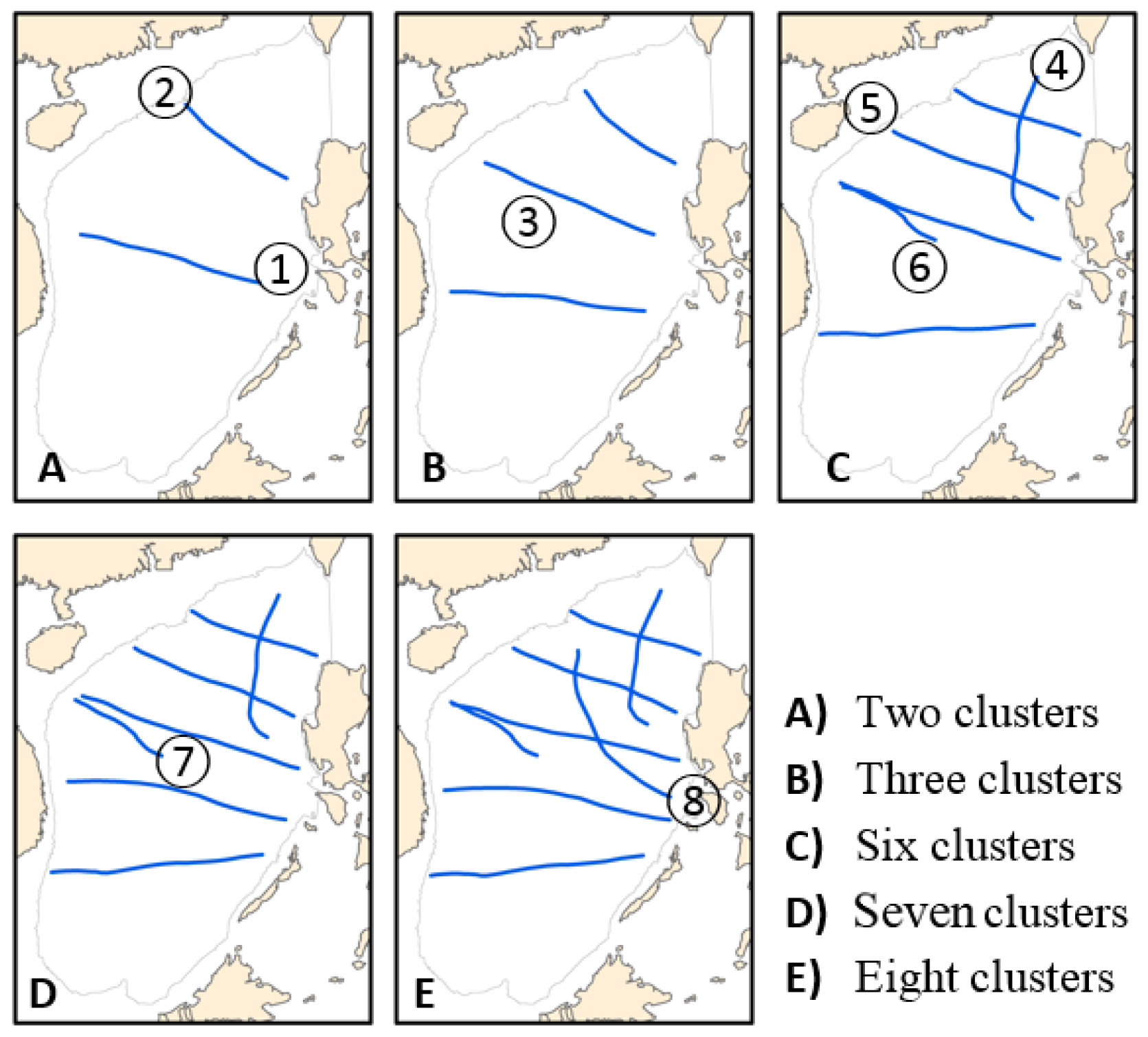
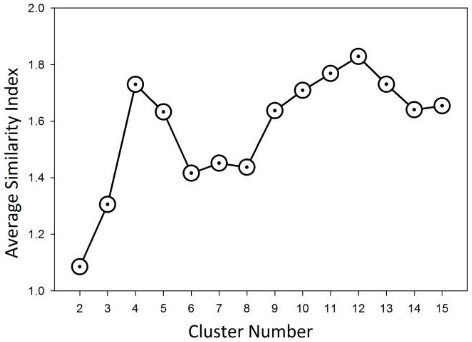
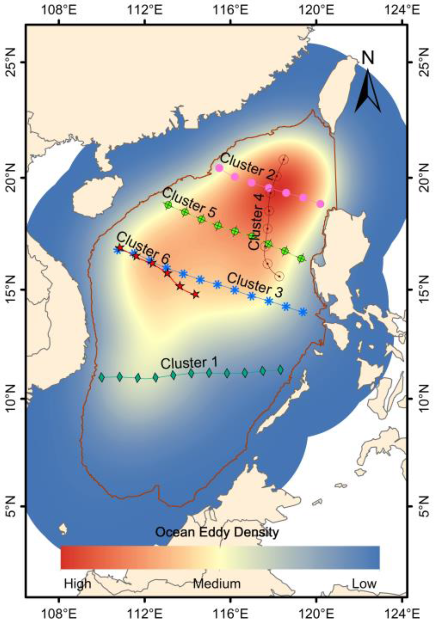
This study examined the distribution of TCs in the SCS and their interrelationships with warm ocean eddies. From 1993 to 2013, we found 134 TCs that interacted with warm ocean eddies for at least a brief period. The tracks of these 134 TCs were grouped into six clusters, most of which are located in the northern SCS.
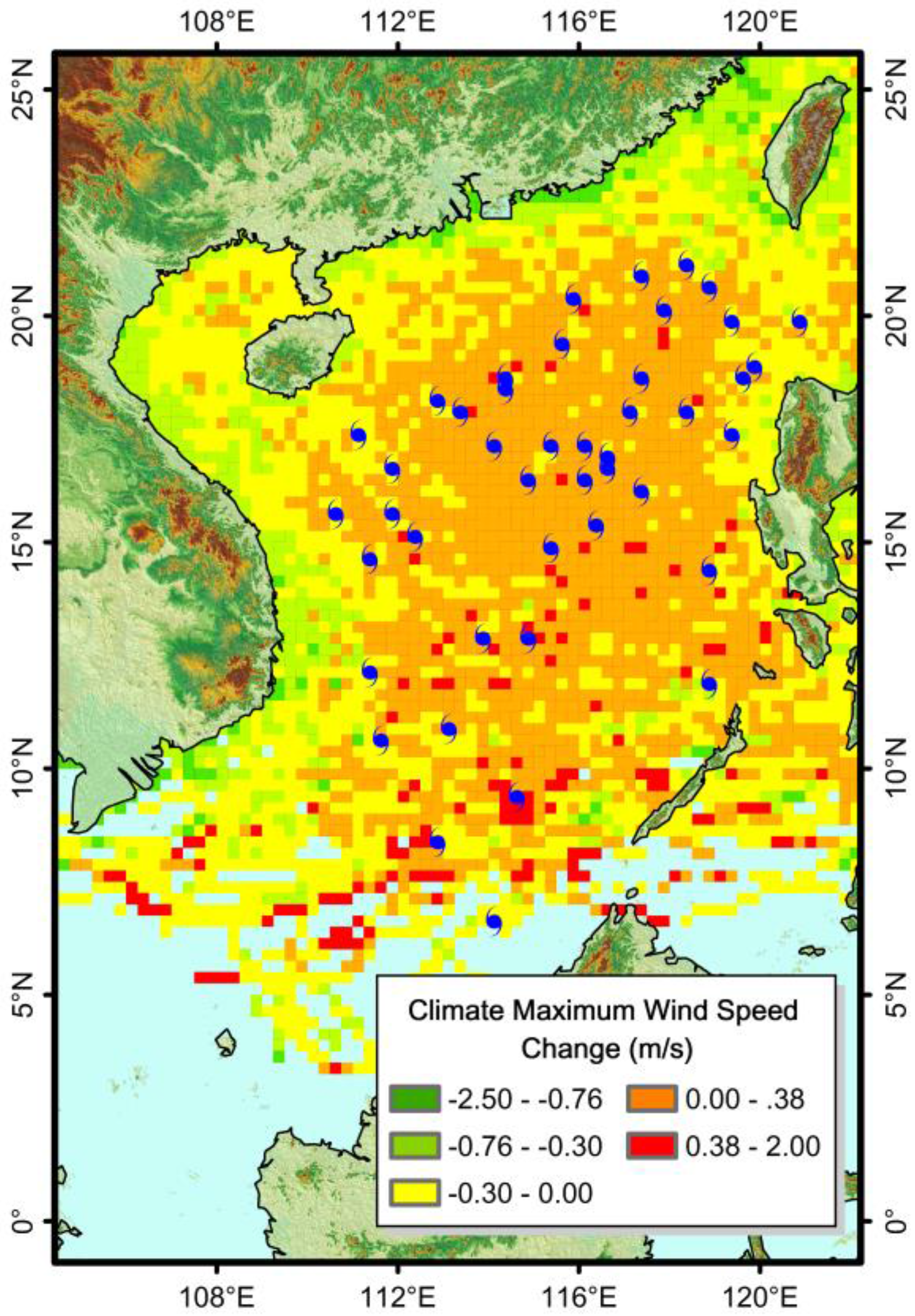
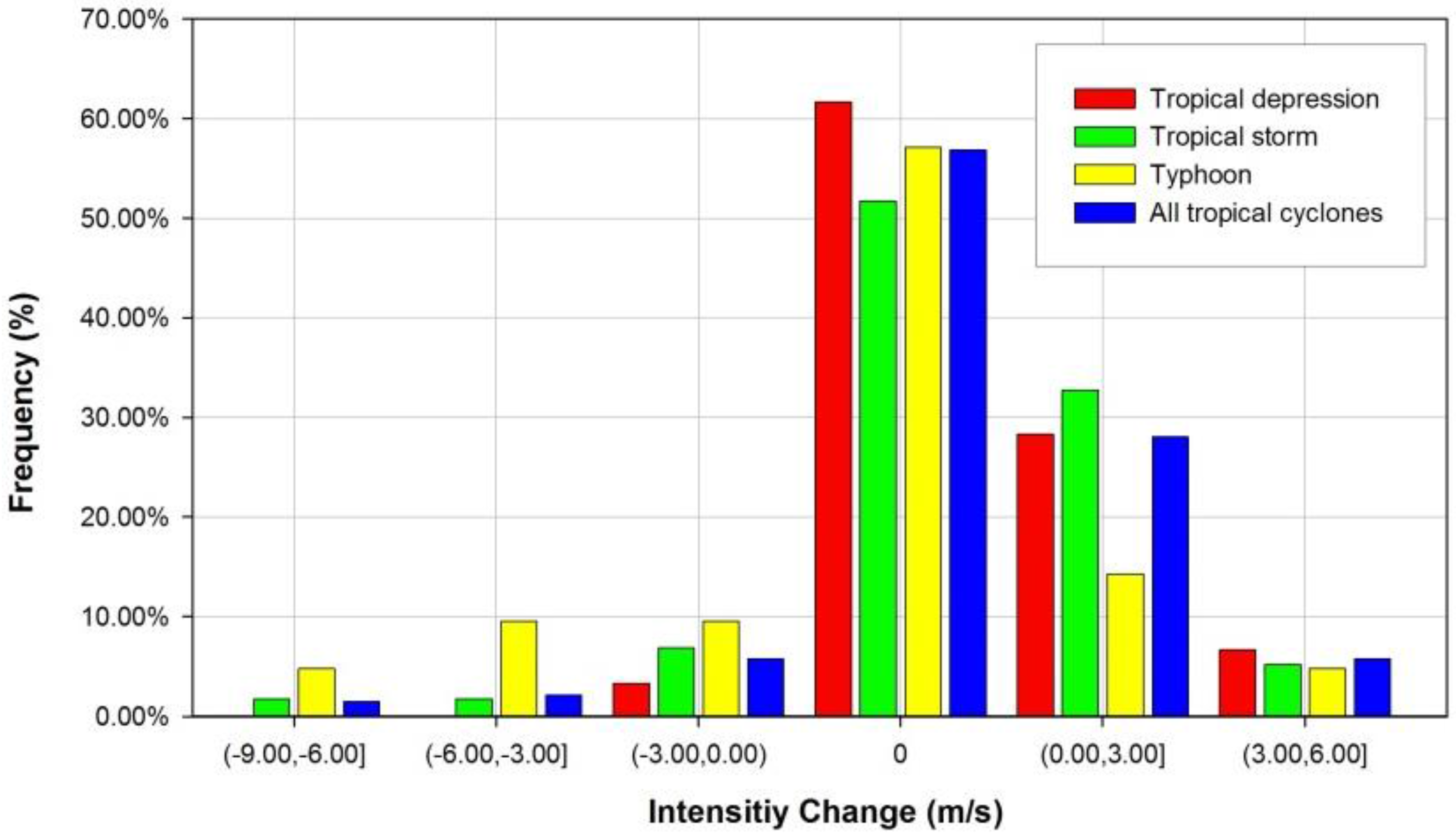
More than half (~57%) of the 134 TCs showed no intensity change after encountering warm ocean eddies in the SCS. Approximately 9% and 34% of the TCs weaken or intensify, respectively, after interacting with a warm ocean eddy. Although the majority of intensifying TCs (~82%) show intensity change values within a narrow range between 0.00 and 3.00 m/s, the difference in intensity is statistically significant.
The intensity change also varies among different categories of TCs. Both tropical storms and depressions tend to intensify more than typhoons; the former two types of TCs tend to have more potential to intensify, whereas the stronger typhoons tend to decay.
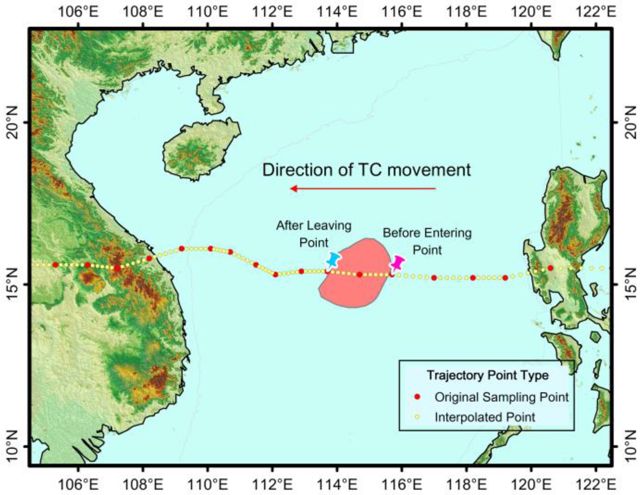
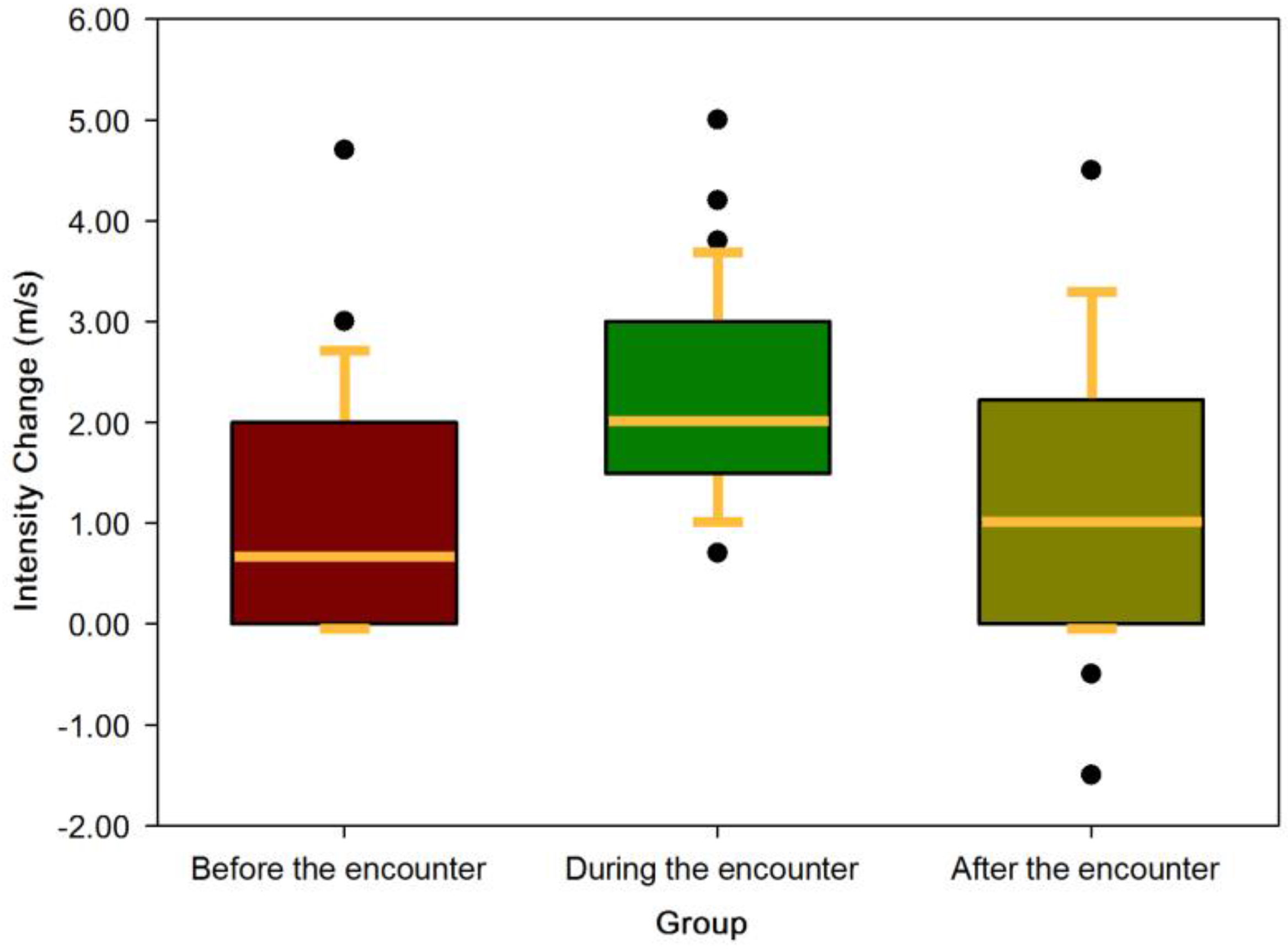
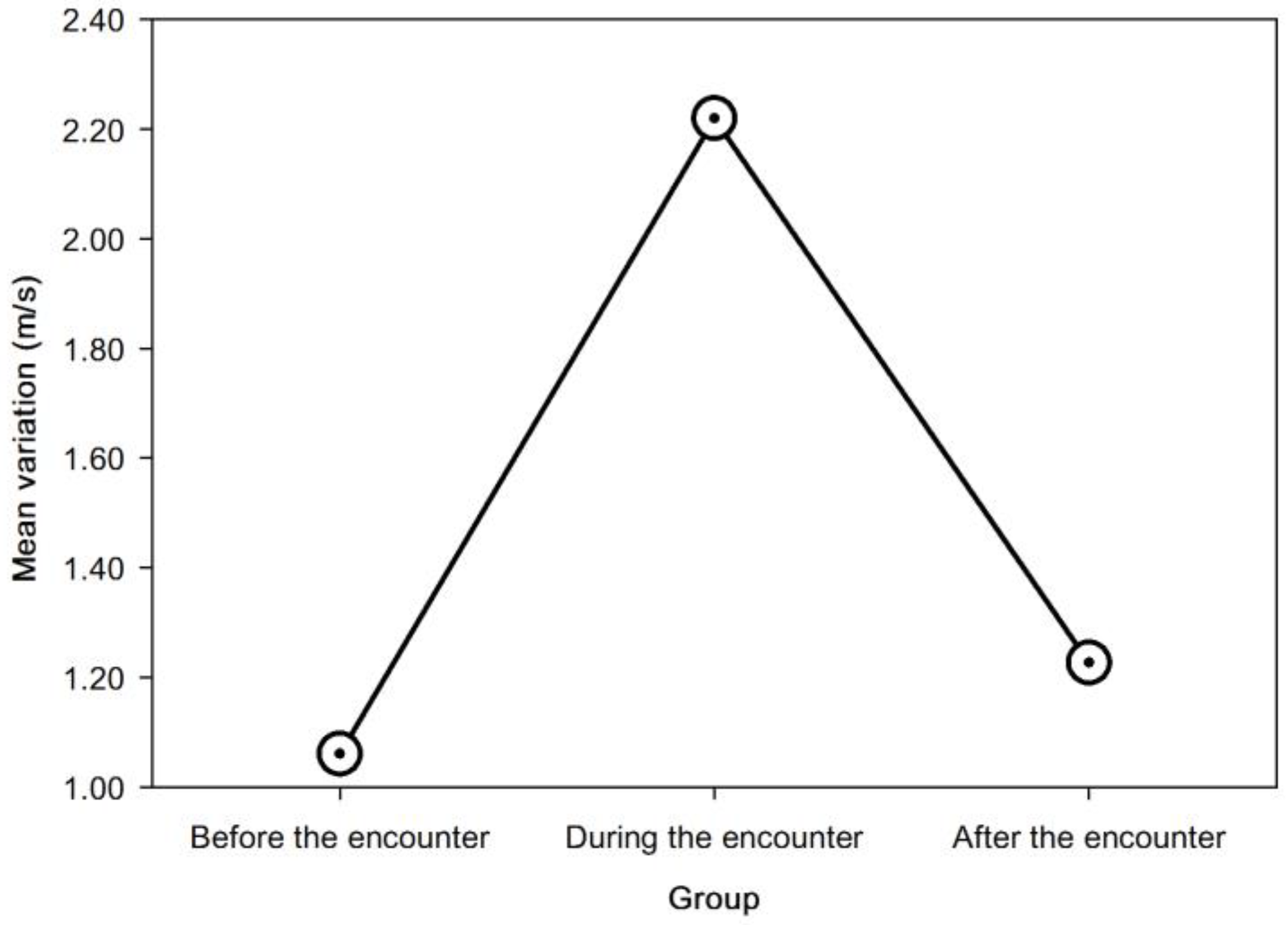
We further examined the temporal variations in TC intensity during the 6-h period before and after a TC meets a warm ocean eddy as well as during the interaction period between a TC and a warm ocean eddy. The differences in intensity changes during these three periods are statistically significant at a 6-h interval but not at a 12-h interval. Consequently, the temporal variations in TC intensity are remarkable only over a short time period—approximately 7 h, which is the average span of interactions between TCs and warm ocean eddies in the SCS.
We also found that the differences in the average SST of warm ocean eddies that encounter intensifying or unchanged TCs as well as those that encounter either weakening or non-weakening TCs are both statistically significant. Moreover, the high mean SST of the warm ocean eddies that encounter intensifying TCs probably indicates that higher SST helps intensify passing TCs. The sizes of warm ocean eddies may also contribute to TC intensifications in the SCS; however, their contribution might be limited due to the relatively small sizes of warm ocean eddies in the SCS compared to the radii of the maximum winds of TCs.

Acknowledgments

This study was funded by the National Science Foundation of China under contract (Grant Number: 41371378) and the National Science Foundation of China (Grant Number: 41421001).

Author Contributions

This research was mainly conducted by Feng Yang, Hui Peng, Yunyan Du and Guofeng Wu. Feng Yang and Hui Peng collected the data; Yunyan Du and Guofeng Wu designed the experiments; Feng Yang performed the experiments, analyzed the data and wrote the manuscript. Hui Peng helped process the data.

Conflicts of Interest

The authors declare no conflicts of interest.

References

  1. Beven, J.L.; Avila, L.A.; Blake, E.S.; Brown, D.P.; Franklin, J.L.; Knabb, R.D.; Pasch, R.J.; Rhome, J.R.; Stewart, S.R. Atlantic hurricane season of 2005. Mon. Weather Rev. 2008, 136, 1109–1173. [Google Scholar] [CrossRef]
  2. Kang, S.-W.; Jun, K.-C.; Park, K.-S.; Han, S.-D. Storm surge hindcasting of Typhoon Maemi in Masan Bay, Korea. Mar. Geod. 2009, 32, 218–232. [Google Scholar] [CrossRef]
  3. McPhaden, M.J.; Foltz, G.R.; Lee, T.; Murty, V.S.N.; Ravichandran, M.; Vecchi, G.A.; Vialard, J.; Wiggert, J.D.; Yu, L. Ocean-atmosphere interactions during Cyclone Nargis. EOS Trans. Am. Geophys. Union 2009, 90, 53–54. [Google Scholar] [CrossRef]
  4. Webster, P.J. Myanmar’s deadly daffodil. Nat. Geosci. 2008, 1, 488–490. [Google Scholar] [CrossRef]
  5. Gopalakrishnan, S.G.; Goldenberg, S.; Quirino, T.; Zhang, X.; Marks, F.M., Jr.; Yeh, K.-S.; Atlas, R.; Tallapragada, V. Toward improving high-resolution numerical hurricane forecasting: Influence of model horizontal grid resolution, initialization, and physics. Weather Forecast. 2012, 27, 647–666. [Google Scholar] [CrossRef]
  6. DeMaria, M.; Mainelli, M.; Shay, L.K.; Knaff, J.A.; Kaplan, J. Further improvements to the Statistical Hurricane Intensity Prediction Scheme (SHIPS). Weather Forecast. 2005, 20, 531–543. [Google Scholar] [CrossRef]
  7. Holliday, C.R.; Thompson, A.H. Climatological characteristics of rapidly intensifying typhoons. Mon. Weather Rev. 1979, 107, 1022–1034. [Google Scholar] [CrossRef]
  8. Kaplan, J.; Demaria, M. Large-Scale Characteristics of rapidly intensifying tropical cyclones in the North Atlantic Basin. Weather Forecast. 2003, 18, 1093–1108. [Google Scholar] [CrossRef]
  9. Krishnamurti, T.N.; Pattnaik, S.; Stefanova, L.; Kumar, T.; Mackey, B.P.; O’Shay, A.J.; Pasch, R.J. The hurricane intensity issue. Mon. Weather Rev. 2005, 133, 1886–1912. [Google Scholar] [CrossRef]
  10. Lin, I.-I.; Goni, G.J.; Knaff, J.A.; Forbes, C.; Ali, M. Ocean heat content for tropical cyclone intensity forecasting and its impact on storm surge. Nat. Hazards 2013, 66, 1481–1500. [Google Scholar] [CrossRef]
  11. Sun, Y.; Zhong, Z.; Yi, L.; Ha, Y.; Sun, Y. The opposite effects of inner and outer sea surface temperature on tropical cyclone intensity. J. Geophys. Res. Atmos. 2014, 119, 2193–2208. [Google Scholar] [CrossRef]
  12. Shay, L.K.; Goni, G.J.; Black, P.G. Effects of a warm oceanic feature on hurricane opal. Mon. Weather Rev. 2000, 128, 1366–1383. [Google Scholar] [CrossRef]
  13. Hong, X.; Chang, S.W.; Raman, S.; Shay, L.K.; Hodur, R. The interaction between hurricane opal (1995) and a warm core ring in the Gulf of Mexico. Mon. Weather Rev. 2000, 128, 1347–1365. [Google Scholar] [CrossRef]
  14. Goni, G.J.; Trinanes, J.A. Ocean thermal structure monitoring could aid in the intensity forecast of tropical cyclones. EOS Trans. Am. Geophys. Union 2003, 84, 573–578. [Google Scholar] [CrossRef]
  15. Emanuel, K.; DesAutels, C.; Holloway, C.; Korty, R. Environmental control of tropical cyclone intensity. J. Atmos. Sci. 2004, 61, 843–858. [Google Scholar] [CrossRef]
  16. Marks, F.D.; Shay, L.K. Landfalling tropical cyclones: Forecast problems and associated research opportunities. Bull. Am. Meteorol. Soc. 1998, 79, 305–323. [Google Scholar]
  17. Namias, J.; Cayan, D.R. Large-scale air-sea interactions and short-period climatic fluctuations. Science 1981, 214, 869–876. [Google Scholar] [CrossRef] [PubMed]
  18. Jaimes, B.; Shay, L.K. Mixed layer cooling in mesoscale oceanic eddies during Hurricanes Katrina and Rita. Mon. Weather Rev. 2009, 137, 4188–4207. [Google Scholar] [CrossRef]
  19. Lin, I.-I.; Wu, C.-C.; Emanuel, K.A.; Lee, I.-H.; Wu, C.-R.; Pun, I.-F. The interaction of Supertyphoon Maemi (2003) with a warm ocean eddy. Mon. Weather Rev. 2005, 133, 2635–2649. [Google Scholar] [CrossRef]
  20. Demaria, M.; Kaplan, J. Sea surface temperature and the maximum intensity of Atlantic Tropical Cyclones. J. Clim. 1994, 7, 1324–1334. [Google Scholar] [CrossRef]
  21. Leipper, D.F.; Volgenau, D. Hurricane heat potential of the Gulf of Mexico. J. Phys. Oceanogr. 1972, 2, 218–224. [Google Scholar] [CrossRef]
  22. Wu, C.-C.; Lee, C.-Y.; Lin, I.-I. The effect of the ocean eddy on tropical cyclone intensity. J. Atmos. Sci. 2007, 64, 3562–3578. [Google Scholar] [CrossRef]
  23. Lin, I.-I.; Chou, M.D.; Wu, C.C. The impact of a warm ocean eddy on Typhoon Morakot (2009): A preliminary study from satellite observations and numerical modelling. Terr. Atmos. Ocean. Sci. 2011, 22, 661–671. [Google Scholar] [CrossRef]
  24. Lin, I.-I.; Chen, C.H.; Pun, I.F.; Liu, W.T.; Wu, C.C. Warm ocean anomaly, air sea fluxes, and the rapid intensification of tropical cyclone Nargis (2008). Geophys. Res. Lett. 2009, 36. [Google Scholar] [CrossRef]
  25. Lin, I.-I.; Wu, C.-C.; Pun, I.-F.; Ko, D.-S. Upper-ocean thermal structure and the Western North Pacific Category 5 Typhoons. Part I: Ocean features and the category 5 typhoons’ intensification. Mon. Weather Rev. 2008, 136, 3288–3306. [Google Scholar] [CrossRef]
  26. Lin, I.-I.; Pun, I.-F.; Wu, C.-C. Upper-ocean thermal structure and the Western North Pacific Category 5 Typhoons. Part II: Dependence on translation speed. Mon. Weather Rev. 2009, 137, 3744–3757. [Google Scholar] [CrossRef]
  27. Ali, M.; Jagadeesh, P.; Jain, S. Effects of eddies on Bay of Bengal cyclone intensity. EOS Trans. Am. Geophys. Union 2007, 88, 93–95. [Google Scholar] [CrossRef]
  28. Bender, M.A.; Ginis, I. Real-case simulations of Hurricane–ocean interaction using a high-resolution coupled model: Effects on hurricane intensity. Mon. Weather Rev. 2000, 128, 917–946. [Google Scholar] [CrossRef]
  29. Vianna, M.L.; Menezes, V.V.; Pezza, A.B.; Simmonds, I. Interactions between Hurricane Catarina (2004) and warm core rings in the South Atlantic Ocean. J. Geophys. Res. Oceans 2010, 115. [Google Scholar] [CrossRef]
  30. Chelton, D.B.; Schlax, M.G.; Samelson, R.M. Global observations of nonlinear mesoscale eddies. Prog. Oceanogr. 2011, 91, 167–216. [Google Scholar] [CrossRef]
  31. Chelton, D.B.; Schlax, M.G.; Samelson, R.M.; de Szoeke, R.A. Global observations of large oceanic eddies. Geophys. Res. Lett. 2007, 34. [Google Scholar] [CrossRef]
  32. Chelton, D.B.; Gaube, P.; Schlax, M.G.; Early, J.J.; Samelson, R.M. The influence of nonlinear mesoscale eddies on near-surface oceanic chlorophyll. Science 2011, 334, 328–332. [Google Scholar] [CrossRef] [PubMed]
  33. Liu, F.; Tang, S.; Chen, C. Impact of nonlinear mesoscale eddy on phytoplankton distribution in the northern South China Sea. J. Mar. Syst. 2013, 123–124, 33–40. [Google Scholar] [CrossRef]
  34. Hausmann, U.; Czaja, A. The observed signature of mesoscale eddies in sea surface temperature and the associated heat transport. Deep Sea Res. I Oceanogr. Res. Papers 2012, 70, 60–72. [Google Scholar] [CrossRef]
  35. Ma, Z.H.; Fei, J.F.; Liu, L.; Huang, X.G.; Cheng, X.P. Effects of the cold core eddy on tropical cyclone intensity and structure under idealized air-sea interaction conditions. Am. Meteorol. Soc. 2013, 141, 1285–1303. [Google Scholar] [CrossRef]
  36. Oropeza, F.; Raga, G.B. Rapid deepening of tropical cyclones in the northeastern Tropical Pacific: The relationship with oceanic eddies. Atmósfera 2015, 28, 27–42. [Google Scholar] [CrossRef]
  37. Goni, G.; Kamholz, S.; Garzoli, S.; Olson, D. Dynamics of the Brazil-Malvinas confluence based on inverted echo sounders and altimetry. J. Geophys. Res. Oceans 1996, 101, 16273–16289. [Google Scholar] [CrossRef]
  38. Yi, J.; Du, Y.; He, Z.; Zhou, C. Enhancing the accuracy of automatic eddy detection and the capability of recognizing the multi-core structures from maps of sea level anomaly. Ocean Sci. 2014, 10, 39–48. [Google Scholar] [CrossRef] [Green Version]
  39. Chen, S. Geo-system and geo-information system. Acta Geogr. Sin. 1991, 58, 1–7. (In Chinese) [Google Scholar]
  40. Lopes, S.; Brondino, N.; Rodrigues da Silva, A. GIS-based analytical tools for transport planning: Spatial regression models for transportation demand forecast. ISPRS Int. J. Geo-Inf. 2014, 3, 565–583. [Google Scholar] [CrossRef]
  41. Ford, A.; Barr, S.; Dawson, R.; James, P. Transport accessibility analysis using GIS: Assessing sustainable transport in London. ISPRS Int. J. Geo-Inf. 2015, 4, 124–149. [Google Scholar] [CrossRef]
  42. Holloway, P.; Miller, J. Exploring spatial scale, autocorrelation and nonstationarity of bird species richness patterns. ISPRS Int. J. Geo-Inf. 2015, 4, 783–798. [Google Scholar] [CrossRef]
  43. Tran, C.; Yost, R.; Yanagida, J.; Saksena, S.; Fox, J.; Sultana, N. Spatio-temporal occurrence modeling of highly pathogenic avian influenza subtype H5N1: A case study in the Red River Delta, Vietnam. ISPRS Int. J. Geo-Inf. 2013, 2, 1106–1121. [Google Scholar] [CrossRef]
  44. Jongman, B.; Wagemaker, J.; Romero, B.; de Perez, E. Early flood detection for rapid humanitarian response: Harnessing Near real-time satellite and twitter signals. ISPRS Int. J. Geo-Inf. 2015, 4, 2246–2266. [Google Scholar] [CrossRef]
  45. Zou, L.; Ren, A.; Xu, F.; Zhang, X. Typhoon track forecasting based on GIS spatial analyses. J. Tsinghua Univ. (Sci. Technol.) 2008, 12, 2036–2040. (In Chinese) [Google Scholar]
  46. Chen, S. Source regions of tropical storms over Northwest Pacific Ocean. Meteorological 1990, 16, 23–26. (In Chinese) [Google Scholar]
  47. Yumoto, M.; Matsuura, T. Interdecadal variability of tropical cyclone activity in the Western North Pacific. J. Meteorol. Soc. Jpn. Ser. II 2001, 79, 23–35. [Google Scholar] [CrossRef]
  48. Wang, G.; Su, J.; Chu, P.C. Mesoscale eddies in the South China Sea observed with altimeter data. Geophys. Res. Lett. 2003, 30. [Google Scholar] [CrossRef]
  49. Chen, G.; Hou, Y.; Chu, X. Mesoscale eddies in the South China Sea: Mean properties, spatiotemporal variability, and impact on thermohaline structure. J. Geophys. Res. Oceans 2011, 116. [Google Scholar] [CrossRef]
  50. Wang, G.; Su, J.; Li, R. Mesoscale eddies in the South China Sea and their impact on temperature profiles. Acta Oceanol. Sin. 2005, 24, 39–45. [Google Scholar]
  51. Hu, Z.; Tan, Y.; Song, X.; Zhou, L.; Lian, X.; Huang, L.; He, Y. Influence of mesoscale eddies on primary production in the South China Sea during spring inter-monsoon period. Acta Oceanol. Sin. 2014, 33, 118–128. [Google Scholar] [CrossRef]
  52. Liu, G.-P.; Hu, J.-Y. Response of the mesoscale eddies to tropical cyclones in the South China Sea: A case study. J. Oceanogr. Taiwan Strait 2009, 28, 308–315, (In Chinese with English Abstract). [Google Scholar]
  53. Yuan, D.; Han, W.; Hu, D. Surface Kuroshio path in the Luzon Strait area derived from satellite remote sensing data. J. Geophys. Res. Oceans 2006, 111. [Google Scholar] [CrossRef]
  54. Lin, P.-F.; Wang, F.; Chen, Y.-L.; Tang, X.-H. Temporal and spatial variation characteristics on eddies in the South China Sea: I Statistical analyses. Acta Oceanol. Sin. 2007, 29, 14–22, (In Chinese with English Abstract). [Google Scholar]
  55. Ying, M.; Zhang, W.; Yu, H.; Lu, X.; Feng, J.; Fan, Y.; Zhu, Y.; Chen, D. An Overview of the China Meteorological Administration Tropical Cyclone Database. J. Atmos. Ocean. Technol. 2014, 31, 287–301. [Google Scholar] [CrossRef]
  56. Liang, J.; Ren, F.-M.; Yang, X.-Q. Study on the differences between CMA and JTWC tropical cyclone datasets for northwest Pacific. Acta Oceanol. Sin. 2010, 32, 10–22. (In Chinese) [Google Scholar]
  57. Okubo, A. Horizontal dispersion of floatable particles in the vicinity of velocity singularities such as convergences. Deep Sea Res. Oceanogr. Abstr. 1970, 17, 445–454. [Google Scholar] [CrossRef]
  58. Weiss, J. The dynamics of enstrophy transfer in two-dimensional hydrodynamics. Phys. D Nonlinear Phenom. 1991, 48, 273–294. [Google Scholar] [CrossRef]
  59. Bezdek, J.C.; Ehrlich, R.; Full, W. FCM: The fuzzy c-means clustering algorithm. Comput. Geosci. 1984, 10, 191–203. [Google Scholar] [CrossRef]
  60. Chu, H.-J.; Liau, C.-J.; Lin, C.-H.; Su, B.-S. Integration of fuzzy cluster analysis and kernel density estimation for tracking typhoon trajectories in the Taiwan region. Expert Syst. Appl. 2012, 39, 9451–9457. [Google Scholar] [CrossRef]
  61. Kim, H.S.; Kim, J.H.; Ho, C.H.; Chu, P.S. Pattern classification of typhoon tracks using the fuzzyc-means clustering method. J. Clim. 2011, 24, 488–508. [Google Scholar] [CrossRef]
  62. Davies, D.L.; Bouldin, D.W. A cluster separation measure. IEEE Trans. Pattern Anal. Mach. Intell. 1979, 2, 224–227. [Google Scholar] [CrossRef]
  63. Camargo, S.J.; Robertson, A.W.; Gaffney, S.J.; Smyth, P.; Ghil, M. Cluster analysis of typhoon tracks. Part I: General properties. J. Clim. 2007, 20, 3635–3653. [Google Scholar] [CrossRef]
  64. Li, C.-H.; Liu, C.-X.; Cheng, Z.-Q. The characteristics of temporal and spatial distribution of tropical cyclone frequencies over the South China Sea and its affecting oceanic factors in the past 50 yrs. J. Trop. Meteorol. 2007, 23, 341–347. (In Chinese) [Google Scholar]
  65. Harr, P.A.; Elsberry, R.L. Large-Scale Circulation Variability over the Tropical Western North Pacific. Part I: Spatial Patterns and Tropical Cyclone Characteristics. Mon. Weather Rev. 1995, 123, 1225–1246. [Google Scholar] [CrossRef]
  66. Willoughby, H.E.; Clos, J.A.; Shoreibah, M.G. Concentric eye walls, secondary wind maxima, and the evolution of the hurricane vortex. J. Atmos. Sci. 1982, 39, 395–411. [Google Scholar] [CrossRef]
  67. Shu, S.; Ming, J.; Chi, P. Large-Scale Characteristics and Probability of Rapidly Intensifying Tropical Cyclones in the Western North Pacific Basin. Weather Forecast. 2012, 27, 411–423. [Google Scholar] [CrossRef]
  68. Xiu, P.; Chai, F.; Shi, L.; Xue, H.; Chao, Y. A census of eddy activities in the South China Sea during 1993–2007. J. Geophys. Res. Oceans 2010, 115. [Google Scholar] [CrossRef]
  69. Emanuel, K.A. The maximum intensity of hurricanes. J. Atmos. Sci. 1988, 45, 1143–1155. [Google Scholar] [CrossRef]
  70. Ren, X.; Perrie, W. Air-sea interaction of typhoon Sinlaku (2002) simulated by the Canadian MC2 model. Adv. Atmos. Sci. 2006, 23, 521–530. [Google Scholar] [CrossRef]
  71. Zhu, T.; Zhang, D.-L. The impact of the storm-induced SST cooling on hurricane intensity. Adv. Atmos. Sci. 2006, 23, 14–22. [Google Scholar] [CrossRef]
  72. Chan, J.C.L.; Duan, Y.; Shay, L.K. Tropical cyclone intensity change from a simple ocean–atmosphere coupled model. J. Atmos. Sci. 2001, 58, 154–172. [Google Scholar] [CrossRef]
  73. Liu, N.; Ling, T.J.; Wang, H.; Zhang, Y.F.; Gao, Z.Y.; Wang, Y. Numerical simulation of Typhoon Muifa (2011) using a Coupled Ocean-Atmosphere-Wave-Sediment Transport (COAWST) modeling system. J. Ocean Univ. China 2015, 14, 199–209. [Google Scholar] [CrossRef]
  74. DeMaria, M.; Kaplan, J. A Statistical Hurricane Intensity Prediction Scheme (SHIPS) for the Atlantic Basin. Weather Forecast. 1994, 9, 209–220. [Google Scholar] [CrossRef]
  75. Miyamoto, Y.; Takemi, T. An effective radius of the sea surface enthalpy flux for the maintenance of a tropical cyclone. Atmos. Sci. Lett. 2010, 11, 278–282. [Google Scholar] [CrossRef]
Figure 1. A flowchart showing how the interacting tropical cyclones (TCs) and warm ocean eddies were selected in this study.
Ijgi 05 00169 g001
Figure 2. A schematic diagram showing how the TC track points were generated and used to calculate TC intensity variations before and after the eddy interaction. The red area in the center of the map represents the sea surface region extracted from a sea level anomaly map that belongs to a warm ocean eddy. The yellow line shows the TC tracks.
Ijgi 05 00169 g002
Figure 3. Distribution of TC tracks in the SCS from 1993 to 2013.
Ijgi 05 00169 g003
Figure 4. Average similarity index with various numbers of clusters using FCM.
Ijgi 05 00169 g004
Figure 5. Clustering results after grouping the TC tracks into three, six, seven, and eight clusters.
Ijgi 05 00169 g005
Figure 6. The FCM clustering results. The orange line shows the 200-m depth isoline of the SCS. The background color shows the density of warm ocean eddies that the TCs encountered.
Ijgi 05 00169 g006
Figure 7. The frequency of TCs in different categories that show no change, an intensifying change, and a weakening change in intensity.
Ijgi 05 00169 g007
Figure 8. Cell-based average of the variations in maximum wind speed along TCs from 1949 to 2013. The blue dots show warm ocean eddies that encountered intensifying TCs in the South China Sea.
Ijgi 05 00169 g008
Figure 9. A box plot diagram showing the changes in TC intensity during the stages before, during, and after TC interactions with warm ocean eddies.
Ijgi 05 00169 g009
Figure 10. The mean value of the changes of TC intensity within a 6-h span before, during, and after interactions between TCs and warm ocean eddies.
Ijgi 05 00169 g010
Table 1. Different TC categories based on the maximum wind scale and maximum sustained surface wind speed.
TC ClassificationMaximum Sustained Surface Wind Speed (m/s)Maximum Wind Scale
Tropical Depression10.8–17.16–7
Tropical Storm17.2–24.48–9
Severe Tropical Storm24.5–32.610–11
Typhoon32.7–41.412–13
Severe Typhoon41.5–50.914–15
Super Typhoon≥51.0≥16
Table 2. The numbers and percentages of TCs that were grouped into the six different clusters by their tracks. The mean distances of all clusters are also provided.
Cluster NumberCluster 1Cluster 2Cluster 3Cluster 4Cluster 5Cluster 6
Number of Members152930202515
Percent (%)11.1921.6422.3914.9318.6611.19
Mean distance (km)1066.02752.471023.811161.06785.711216.43
Table 3. Duncan’s pairwise comparison results.
Cluster NumberMembersSubsets Classification (α = 0.05)
12
229752.473
525785.711
3301023.8071023.807
1151066.0161066.016
420 1161.061
615 1216.434
Significance level 0.0770.289
Table 4. T-test results for changes in TC intensity.
Mean ValueStandard DeviationtdfSig. (Two-Tailed Test)
Intensity change0.48 (m/s)1.783.1971380.002
Table 5. Statistical results of intensity changes (ΔV) for tropical depressions, tropical storms, typhoons, and all TCs. N is the number of TCs. The mean, standard deviation (std. dev), minimum (min), and maximum (max) of ΔV are also provided.
Intensity ClassNMean (m/s)Min (m/s)Max (m/s)Std. Dev (m/s)
Tropical Depressions600.82−1.005.001.32
Tropical Storms580.51−7.004.201.85
Typhoons21−0.55−8.303.302.34
All TCs1390.48−8.305.001.78
Table 6. Statistics of the radius of the maximum wind of TCs and the size of warm ocean eddies: R e ¯ is the average value of the equivalent radius of warm ocean eddies and R w ¯ is the average value of the radius of maximum wind of TCs that interact with warm ocean eddies.
Categories of TC ChangeNMean RatioMax RatioMin Ratio R e ¯ (km) R w ¯ (km)
Intensifying212.024.590.7095.4654.18
Maintenance251.645.180.6372.1954.39
Weakening81.081.620.6251.5550.94
Table 7. The differences in maximum wind speed changes within a 6-h span before, during, and after interactions between TCs and warm ocean eddies.
Sum of SquaresdfMean SquareFSig.
Between groups35.853217.92713.1370.000
Within groups180.1231321.365
Sum215.976134
Table 8. T-test results showing the differences in maximum wind speed changes within a 6-h span before, during, and after interactions between TCs and warm ocean eddies.
GroupDifference (I − J)Standard ErrorSig.95% Confidence Interval
(I) Group(J) GroupLower BoundUpper Bound
During encounterBefore interaction1.1600.2480.0000.6691.650
After interaction0.9930.2420.0000.5141.472
Table 9. T-test analysis of the differences in SST of the warm ocean eddies that encounter non-weakening and weakening TCs and of the warm ocean eddies that encounter intensifying and unchanged TCs. Correlation coefficients (r) between SST and change of TC intensity in these two groups are also presented.
GroupCategories of TC Change#Worm Ocean Eddy SST Mean (°C)Sig. of TestrSig. of Correlation
Group oneNon-weakening11928.480.0210.250.004
Weakening1327.64
Group twoIntensifying4628.720.0340.190.034
unchanged7328.33

