Visual-LiDAR Odometry Aided by Reduced IMU

Abstract

This paper proposes a method for combining stereo visual odometry, Light Detection And Ranging (LiDAR) odometry and reduced Inertial Measurement Unit (IMU) including two horizontal accelerometers and one vertical gyro. The proposed method starts with stereo visual odometry to estimate six Degree of Freedom (DoF) ego motion to register the point clouds from previous epoch to the current epoch. Then, Generalized Iterative Closest Point (GICP) algorithm refines the motion estimation. Afterwards, forward velocity and Azimuth obtained by visual-LiDAR odometer are integrated with reduced IMU outputs in an Extended Kalman Filter (EKF) to provide final navigation solution. In this paper, datasets from KITTI (Karlsruhe Institute of Technology and Toyota technological Institute) were used to compare stereo visual odometry, integrated stereo visual odometry and reduced IMU, stereo visual-LiDAR odometry and integrated stereo visual-LiDAR odometry and reduced IMU. Integrated stereo visual-LiDAR odometry and reduced IMU outperforms other methods in urban areas with buildings around. Moreover, this method outperforms simulated Reduced Inertial Sensor System (RISS), which uses simulated wheel odometer and reduced IMU. KITTI datasets do not include wheel odometry data. Integrated RTK (Real Time Kinematic) GPS (Global Positioning System) and IMU was replaced by wheel odometer to simulate the response of RISS method. Visual Odometry (VO)-LiDAR is not only more accurate than wheel odometer, but it also provides azimuth aiding to vertical gyro resulting in a more reliable and accurate system. To develop low-cost systems, it would be a good option to use two cameras plus reduced IMU. The cost of such a system will be reduced than using full tactical MEMS (Micro-Electro-Mechanical Sensor) based IMUs because two cameras are cheaper than full tactical MEMS based IMUs. The results indicate that integrated stereo visual-LiDAR odometry and reduced IMU can achieve accuracy at the level of state of art.

1. Introduction

Stand-alone stereo visual odometer, LiDAR odometer and Inertial Measurement Unit provide 6-DOF (Degree Of Freedom) state estimation. However, the drawbacks using each sensor alone, motivate the researchers to integrate those sensors. IMUs, especially MEMS (Micro-Electro-Mechanical Sensor) based ones, accumulate errors very rapidly. Visual odometry requires moderate lighting conditions, and it suffers from various error sources in images, such as noise, motion blur, and distortion. The visual measurements are also ambiguous in featureless, self-similar or dynamic environments or during rapid motion which causes many mismatches in the corresponding image points [1]. In LiDAR odometry, the position of range finder is estimated by matching two different scans which are collected at consecutive epochs. ICP (Iterative Closest Point), is one of the most dominant algorithms to find translation and rotation between two point clouds in order to match them by iteratively finding the closest points [2]. ICP algorithms, accumulate error over time, and it is prone to be erroneous under fast motion; furthermore, it fails, if the point clouds are very sparse, especially in suburban areas where two sides of the road are covered with vegetation. ICP algorithms always converge to the local minimum. Therefore, it needs a good initial guess of transformation to converge to the global minimum [3]. Another problem of ego motion estimation by moving the LiDAR odometer, involves motion distortion in point clouds due to the different receiving time of the range measurements [4]. Stereo cameras and LiDAR can be complementary sensors. Stereo VO (Visual Odometry) not only gives a good initial guess for ICP algorithm but also helps compensating the motion distortion. We assume that velocity and angular velocity are constant during the scanning period. Then, we can calculate the transformation of each point of the point cloud to the first point coordinate system of the point cloud using stereo VO rotation and translation. Afterwards, ICP will refine the initial transformation.

A new integration method for stereo visual-LiDAR odometry and 3D (Three-Dimensional) reduced IMU is proposed in this paper. The wheel odometer in RISS (Reduced Inertial Sensor System), which was proposed by Noureldin et al. [5], is replaced by a stereo visual-LiDAR odometer. The integrated stereo visual-LiDAR odometry and reduced IMU consists of two accelerometers in the x and y directions, one gyroscope in the z direction and two cameras and LiDAR. The horizontal accelerometers determine roll and pitch. Vertical gyro is used for azimuth determination and two cameras and LiDAR measure displacement and rotation between two consecutive LiDAR coordinate systems. This system outperforms simulated RISS. Stereo visual-LiDAR odometer provides not only the translation, but also the rotation between two LiDAR coordinate systems at consecutive epochs. Therefore, we can calculate the visual-LiDAR azimuth at each epoch by estimating the transformation between the LiDAR coordinate system, the IMU coordinate system and the navigation frame at the first epoch. The visual-LiDAR azimuth is integrated with the initial azimuth (which is obtained by vertical gyro’s output, forward translation obtained from visual-LiDAR odometer and roll and pitch) by Kalman Filter (KF) resulting in more accurate vehicle azimuth with less number of spikes. To sum up, stereo VO-LiDAR is not only more accurate than wheel odometer, but it also provides azimuth aiding to vertical gyro solution.

The paper is organized as follows: Previous works are addressed in Section 2. Section 3 introduces an integrated visual-Lidar odometry and reduced IMU methodology, the results and analysis are provided in Section 4. Conclusion and discussion are given in Section 5. Finally, future work is given in Section 6.

2. Previous Works

In this section, previous works in visual odometry, LiDar odometry and sensor integration are described.

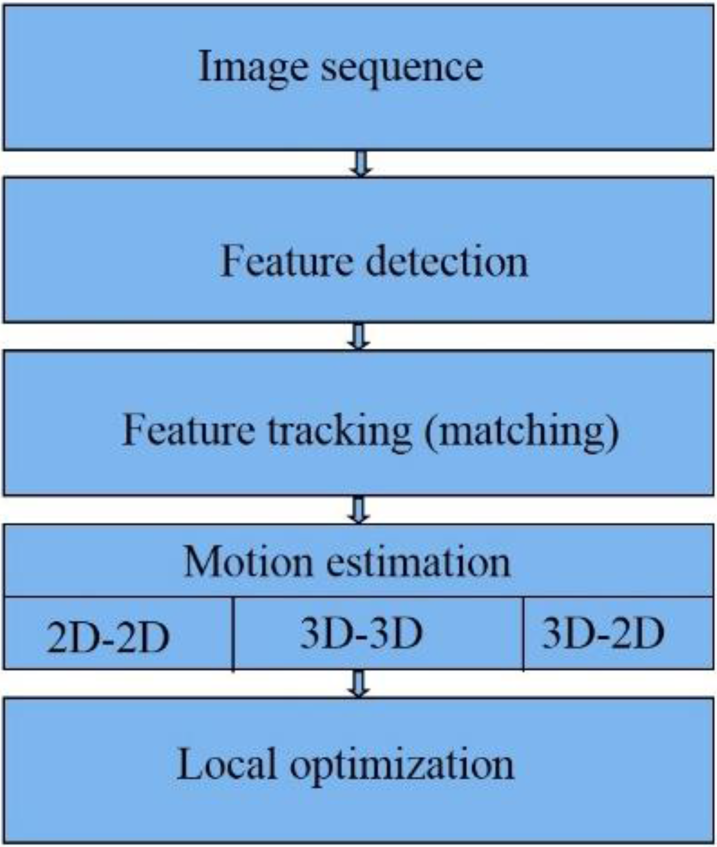
2.1. Visual Odometry

The key idea of visual odometry is to estimate the motion of a vehicle or robot by visually tracking landmarks using an on-board camera [1]. In other words, the 6 degrees of freedom (6DoF) ego-motion estimation (including three position increments and three alignment increments), merely from image measurements is called visual odometry [6]. This technique is considered as a dead reckoning (DR) approach. Therefore, a visual odometer is a relative positioning system with position and alignment increments estimated at each epoch. Similar to a DR system, visual odometry accumulates errors over time [1], and it suffers from various error sources in images such as noise, motion blur and distortion. The visual measurements are also ambiguous in featureless, self-similar or dynamic environments and during rapid motion, which causes many mismatches in the corresponding image points. The following assumptions are made for visual odometry [7]:

(1)

There is sufficient illumination in the environment

(2)

Static objects in the image dominates over moving objects

(3)

There is enough texture to allow apparent motion to be extracted

(4)

There is sufficient scene overlap between consecutive frames

Visual odometry is a particular case of Structure from Motion (SfM). VO focuses on camera pose estimation from sequential images. SfM, which is more general than VO, focuses on both camera pose estimation and 3D scene point reconstruction [7]. Sometimes, SfM is used as a synonym of SLAM (Simultaneous Localization And Mapping). SLAM, enables the ALV (Autonomous Land Vehicle) to build a map of environment while it simultaneously uses this map to estimate the vehicle pose [8]. Many different types of SLAM are known. Sonar, laser range and visual SLAM are the most commonly used [9].

Visual navigation is likely to become a widely used navigation solution because cameras are already common on robots, laptops, smartphones and tablets. Cameras are also relatively cheap and they do not interfere with other sensors. Furthermore, Cameras are not easily misled and require no additional infrastructure. In theory, visual odometry can work in any environment where there is enough light and texture that static features can be identified. One main advantage of visual odometry is the high accuracy compared to wheel speed sensors, especially in slippery terrains where wheel speed sensors often yield low accuracy performance [6]. The wheel odometer measures distances travelled by the vehicle. On slippery ground, a wheel odometer cannot provide accurate forward velocity. In addition, a wheel odometer shows the measured distances per second at turnings (where the vehicle’s wheel direction is not parallel with the vehicle’s forward direction) instead of vehicle’s forward velocity which is used in a reduced inertial sensor mechanization. The visual odometry drift rates are mostly smaller than the drift rates of low-cost MEMS based IMUs, especially when the vehicle is static or has low dynamics [6].

A lot of visual odometry algorithms have been developed for monocular, binocular (stereo) and multi-ocular cameras. Further subdivision is possible into methods using feature tracking over a whole sequence of images and methods that are matching features between consecutive images [6]. Binocular and multi-ocular cameras yield better results because they do not suffer from scale ambiguities. In stereo visual odometry, we can perform triangulation followed by resectioning repeatedly [1]. There are also other methods for which the recovery of the three-dimensional scene structure is not needed [6]. A lot of methods have been developed for finding mismatches and detecting outliers. Kitt et al. [6] proposed a bucketing technique combined with the RANSAC (RANdom Sample Consensus) based outlier rejection .

Figure 1 summarizes the major steps in visual odometry steps [9] which will be described in the following.

Figure 1. Visual Odometry steps.

Figure 1. Visual Odometry steps.

The first step in VO is capturing image sequences. The next step is feature extraction, Features are special points which can stably be re-detected from later images, taken from another point of view [9]. In Feature matching (or tracking), we will find correspondences between features in the current frame with features in previous frames [9,10]. There are several methods for motion estimation [7], e.g., 2D-to-2D, 3D-to-3D and 3D-to-2D methods. Compared to the other two methods for stereo VO, 3D-to-2D, drifts slower and gives more accurate results [7]. We can optimize the estimated rotation and translation between the camera coordinate systems using optimization methods including windowed camera pose estimation, Bundle Adjustment (BA), Bucketing and Loop closure [11].

In this paper, we implemented a 3D-to-2D VO algorithm. We used windowed processing, bucketing and bundle adjustment to reduce growth rate of the VO errors.

2.2. LiDAR Odometry

LiDAR has become a useful range sensor in Automatic Vehicle Localization (AVL) and robot navigation. Several methods have been developed during the last two decades to find transformation between two point clouds. A feature based registration method can be used to find initial transformation between two point clouds. This method finds several keypoints in each point cloud and computes descriptors for each keypoint. The next step is matching. The corresponding keypoints are found using keypoint descriptors. In order to obtain better results, the mismatches have to be found. RANSAC based methods can be used in order to reduce the effect of undetected mismatches. As the final step, the rotation and translation between corresponding keypoints are calculated [12].

NDT (Normal Distribution Transform) is another method for point cloud registration. NDT uses standard optimization techniques which are applied to statistical models of 3D points to determine the most probable registration between two point clouds [13].

ICP (Iterative Closest Point) is one of the most dominant algorithms for LiDAR odometry and has become the most widely used method for aligning point clouds [2]. ICP converges to local minima, and it is based on minimizing the squared error. Several versions of the ICP method have been developed during the last decade. In point-to-point ICP, each point in the first point cloud is paired with the closest point in the second point cloud to form correspondence pairs. The next step is iteratively finding the rotation and translation by minimizing sum of the squared distance between points in each correspondence pair [14]. Equation (1) shows the point-to-point ICP objective function [12]:

$$\underset{R,T}{\min }{\displaystyle \sum }_{X_i}{\left|\left|\left(R{X}_i+T-Y_i\right)\right|\right|}^2$$

(1)

where T and R are the translation vector and rotation matrix between two point sets, $X_i$ is the point in the first point cloud and $Y_i$ is the point at the second point cloud.

In the point-to-plane ICP method, the sum of squared distance between each point in the first point cloud and the tangent plane at the corresponding point in the second point cloud is minimized [14]. Equation (2) shows the point-to-plane ICP objective function [12]:

$$\underset{R,T}{\min }{\displaystyle \sum }_{X_i}{\left(\left(R{X}_i+T-Y_i\right).n_{Y_i}\right)}^2$$

(2)

where $n_{Y_i}$ is the normal vector to the surface at point $Y_i$.

Generalized ICP (plane-to-plane ICP) generalizes over point-to-point and point-to-plane ICP method, and it outperforms both point-to-point and point-to-plane ICP [15]. It uses covariance of the local point neighborhoods in order to align underlying surfaces rather than point [12]. This approach is more robust to incorrect correspondences. In this paper, we used Generalized ICP which is implemented in PCL (Point Cloud Library). Equation (3) shows the plane-to-plane ICP objective function [12]:

$$\underset{R,T}{\min }{\displaystyle \sum }_{X_i}{d}_i^t {(C_i^Y+Q{C}_i^X{Q}^t)}^{-1}{d}_i$$

(3)

where $Q=\left(\begin{array}{cc}R& T\\ 0_{3x1}& 1\end{array}\right)$, $d=Y_i-\left(R{X}_i+T\right)$ , $C_i^X$ and $C_i^Y$ are the covariance matrices of the local point neighborhoods.

2.3. Sensor Integration

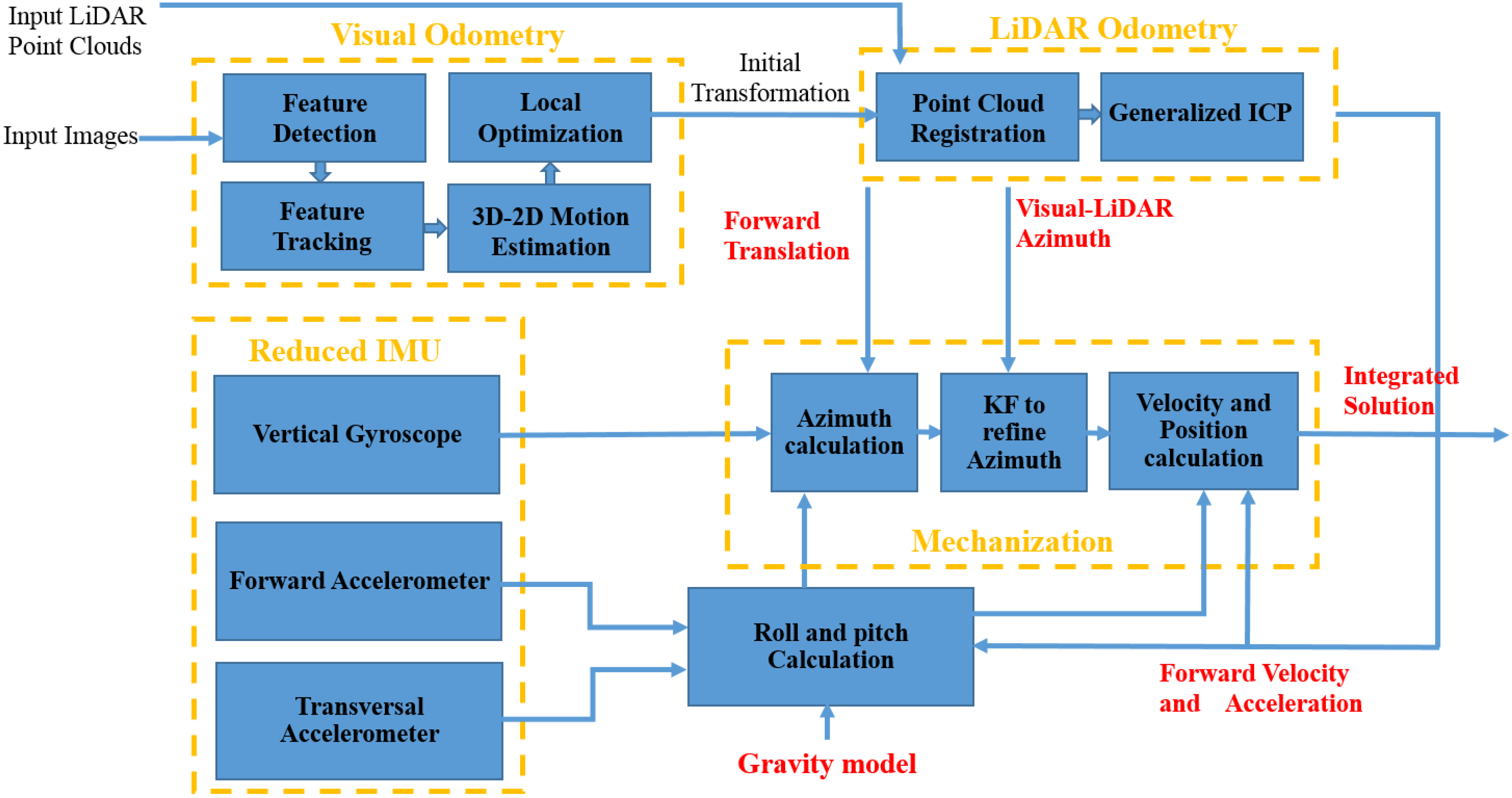
Stand-alone stereo visual odometer, LiDAR odometer and IMU are dead reckoning systems which can provide navigation solution. However, the drawbacks using each sensor alone motivate the researchers to integrate those sensors. IMU and camera are two complementary sensors and several loosely coupled and tightly coupled camera/IMU integration methods have been designed and implemented in the last decade [16,17,18].

Sirtkaya et al. [16] and Kleinert et al. [19] worked on the integration of IMU and monocular camera. The IMU provides the position and attitude information of the system to remove monocular camera depth ambiguity. Nützi et al. [20] suggested the inertial aided monocular SLAM to estimate the absolute scale of a single camera. For loosely coupled integration, the stereo cameras and IMU provide separate navigation solutions independently, making the data fusion more flexible. The inertial predictions in EKF (Extended Kalman Filter) can be corrected by rotation and translation obtained by visual odometry [21]. Similarly, the inertial measurements could also correct the 6 degree-of-freedom (DOF) ego-motion estimated by visual odometry [22]. For tightly coupled integration, the IMU and vision data are processed together to obtain the navigation solution. Tardif et al. [23] suggested a new approach of vision aided inertial navigation. In the proposed method, IMU provides the pseudo gravity measurements when acceleration is low. In [24], the IMU outputs and pixel coordinates in images are used to correct system motion, under certain situations. Using this method, the 3D feature points, expressed in a global coordinate system, are also included in the state vector of the Kalman Filter. This big size of state vector, considerably increases the computational complexity.

Motion estimation and distortion correction become a problem in LiDAR odometry without aiding from other sensors [4]. Scherer et al. [25] registered LiDAR point clouds by state estimation from integrated visual odometry and IMU. Scherer et al. [25] combined visual odometry and LiDAR odometry. In this method, ego motion is first estimated by visual odometry to register point clouds and then LiDAR odometry refines the motion estimation. Visual odometry also helps remove the motion distortion in the point clouds.

Noureldin et al. [5] proposed RISS (Reduced Inertial Sensor System) in which a wheel odometer and a 3D reduced IMU (two horizontal accelerometers and one vertical gyro) are integrated. This method has advantages over using a full IMU. With a full IMU, uncompensated accelerometer and gyro biases cause velocity and position degradation. Uncompensated accelerometer bias $\left(b_f\right)$ introduces errors in velocity as a linear function of time (t) and errors in position which grow as a quadratic function of time [5]:

$$\delta v={{\displaystyle \int }}^{\text{}}{b}_{f}dt=b_{f}t$$

(4)

$$\delta p={{\displaystyle \int }}^{\text{}}\delta vdt=\frac{1}{2}{b}_f{t}^2$$

(5)

where $\delta vand\delta p$ are the errors in velocity and position, respectively. The uncompensated horizontal gyro bias $(b_w)$ introduces roll or pitch error ($\delta \theta$) as follows [26]:

$$\delta \theta ={{\displaystyle \int }}^{\text{}}{b}_{w}dt=b_{w}t$$

(6)

The roll and pitch error will incorrectly project the acceleration vector from the body frame to the local level frame as follows [26]:

$$\delta a=gsin\left(\delta \theta \right)\approx g\delta \theta =g{b}_{w}t$$

(7)

This acceleration error causes velocity error proportional to t² ($\delta v={\int }^{\text{}}{b}_{w}gtdt=\frac{1}{2}{b}_{w}g{t}^2$) and position error proportional to t³ ($\delta p={\int }^{\text{}}\delta vdt={\int }^{\text{}}\frac{1}{2}{b}_{w}g{t}^{2}dt=\frac{1}{6}{b}_{w}g{t}^3$) [23].

Furthermore, the uncompensated vertical gyro bias, $b_{wz}$, causes azimuth error proportional to t, $\delta A={\int }^{\text{}}{b}_{wz}dt=b_{wz}t$ [26].

In RISS, the platform pitch ($p$) and roll (r) are calculated as follows [5]:

$$p={\sin }^{-1}\left(\frac{f^y-a^{od}}{g}\right)$$

(8)

$$\text{r}={\sin }^{-1}(\frac{f^x+v^{od}{w}^z}{g\cos p})$$

(9)

where $f^x$ is acceleration in x direction, $f^y$ is acceleration in y direction, $w^z$ is angular velocity in z direction, g is normal gravity, $v^{od}$ and $a^{od}$ are odometer velocity and odometer acceleration, respectively. Therefore, the roll and pitch error calculated from RISS are not proportional with time t [5]. In addition, the wheel odometer provides velocity rather than the integration of accelerometers’ outputs. The RISS roll and pitch error will therefore project the velocity vector rather than the accelerometer vector from the body frame to the local level frame which causes an error in velocity proportional with t and position error proportional with t². The azimuth error caused by uncompensated vertical gyro bias is the only remaining main source of error in 3D RISS.

3. Methodology

A new integration method for stereo visual-LiDAR odometry and 3D reduced IMU is proposed in this paper. The wheel odometer in RISS, which was proposed by [5], is replaced by the stereo visual-LiDAR odometer. Figure 2 shows a diagram of the software system. The overall system is divided into three sections: visual odometry, LiDAR odometry and reduced IMU section. The stereo visual odometry section estimates frame to frame motion at image frame rate using input stereo images [11]. In this section, feature detection block extracts visual features (we used Harris corner) from left image at epoch t_k. Feature tracking block, tracks the extracted features along the right image at epoch t_k and the left image at epoch t_k+1 (KLT (Kanade-Lucas-Tomasi) tracker was used) [7]. The 3D-to-2D motion estimation block performs the triangulation followed by resectioning. A triangulation method is used to reconstruct the 3D scene points from the 2D feature points on the left and right image at epoch t_k. The camera pose is obtained using reconstructed 3D points at epoch t_k and 2D feature points of the left image at epoch t_k+1 by resectioning (we used P3P (Perspective 3 Point) method) [7]. The feature detection block extracts new feature points if the number of the tracked features is less than a threshold. The local optimization blocks optimizes the ego motion estimation using RANSAC (RANdom SAmple Consensus), windowed camera pose estimation, Bundle Adjustment (BA) and Bucketing. In visual odometry, the tracked points are usually contaminated by outliers; in others words, there are incorrect data associations. The RANSAC method was used in the resectioning part to remove the outliers. We used windowed processing to reduce the growth rate of VO errors. Instead of consecutive triangulation and resectioning, we did the triangulation at the first epoch of the reference frame of each window, followed by resectioning at other frames of the window. The length of each window depends on the number of tracked features. If the number of tracked features is less than the desired threshold, we can define a new reference frame and repeat the above procedure. we used Bundle Adjustment (BA) to improve the camera pose estimation if we have matched features across more than two frames [27]. In stereo vision BA, we have to use LM (Levenberg-Marquardt) method which interpolates between the Gauss-Newton algorithm (GNA) and the method of gradient descent. If we use Gauss–Newton algorithm for bundle adjustment, the normal matrix will be singular so we have to use LM algorithm.

Bucketing is another method which was used in the VO local optimization block. In bucketing, the image is divided into several non-overlapping rectangles. In every rectangle, we select a certain number of features randomly [6]. Bucketing has several benefits; first, the computational complexity is reduced and a smaller number of feature points are processed, which is very important for real time applications [6]. Bucketing guarantees that all the feature points are well distributed along the z axis; therefore, both near and far feature points are used for camera pose estimation [6]. Furthermore, in a dynamic scene, where considerable number of points are detected on moving objects, bucketing helps to filter out some of the points located on the moving objects. Therefore, bucketing reduces the drift rate in visual odometry. We used OpenCV library (C++ version) for feature point detection, feature tracking and feature matching, triangulation and resectioning.

Figure 2. Integrated stereo visual-LiDAR odometry and 3D reduced IMU.

Figure 2. Integrated stereo visual-LiDAR odometry and 3D reduced IMU.

The LiDAR odometry section refines the ego motion estimated by stereo VO. Point cloud registration block aligns point clouds collected at consecutive epochs using VO rotation and translation. VO rotation and translation can be used for LiDAR motion distortion removal as well. We ignored the motion distortion correction because Velodyne HDL-64E was used for data collection which is capable of collecting data that can be used to produce quality maps even while moving. Furthermore, LiDAR data rate is high (10 Hz) while the vehicle velocity was low. In addition, we used half of the data (180 degree) for ICP, which reduces the effect of motion distortion.

We used Point Cloud Library (PCL) for LiDAR odometry. Noisy measurements in the point clouds were removed using statistical analysis techniques. PCL outlier removal is based on the computation of the distribution of a point to neighbor points’ distances in the input dataset. For each point, the mean distance from it to all its neighbors has to be computed. As the next step, all points, whose mean distances are outside an interval defined by the global mean and standard deviation, can be considered as outliers and filtered out from the dataset. We did not use all the point clouds as the input of ICP algorithm. We used 180 degrees of point cloud. We also filtered out the points farther than 20 m. Many of the points in point cloud fall on the ground and are less informative for our purpose. These points are eliminated from the point cloud, using a plane fitting. The SAmple Consensus (SAC) segmentation method, which is implemented in PCL, was used to detect and filter out the ground points. In this method, data points further away than a threshold are filtered, then surface normal at each point are estimated and a plane model is set as the method type of SAC method to find the ground points and filter them out. Now, the consecutive point clouds are ready for the Generalized ICP block which refines the ego motion estimation.

The Reduced IMU section consists of two horizontal accelerometers and one vertical gyroscope. The first step in reduced IMU mechanization is initialization. Initial position (initial latitude, initial longitude and initial height) can be obtained by GPS. In order to obtain the initial attitudes, we will go through alignment process [26]. The initial pitch and initial roll can be obtained by Equations (8) and (9). In the following section, we assume the stereo cameras look forward and they are leveled. The x axis of the camera coordinate system points toward the right direction of the vehicle, the y axis points down and the z axis points toward the forward direction of the vehicle. We assume LiDAR is leveled as well, the x axis of the LiDAR coordinate system points toward forward direction of the vehicle, the y axis points toward the left direction of the vehicle and the z axis points up. The stereo visual-LiDAR odometer estimates the parameters of the translation (T^k) and rotation ($R_k^{k+1}$) between the two consecutive LiDAR frames at epoch k and epoch k+1. The forward displacement and velocity, which are used in mechanization, can be obtained as follows:

$$∆x_k^{VO-LiDAR}$$

(10)

$$v_k^{VO-LiDAR forward}=\frac{∆x_k^{VO}}{∆t}$$

(11)

where: $X=\left(\begin{array}{c}∆x_k^{VO-LiDAR}\\ ∆y_k^{VO-LiDAR}\\ ∆z_k^{VO-LiDAR}\end{array}\right)=-{\left(R_k^{k+1}\right)}^{-1}{T}^k$.

The initial azimuth can be obtained by GPS velocity, $A_0={\tan }^{-1}(\frac{v_{GPS}^E}{v_{GPS}^N})$ [5]. After the initialization, the roll, pitch and azimuth, velocity and position can be calculated for each epoch. The Equations (8) and (9) can be applied to calculate the pitch and roll respectively while the azimuth is calculated using the following Equation (5):

$$A_k={\tan }^{-1}(\frac{U^E}{U^N})+w^e\sin {\phi }_{k-1}∆t+\frac{ ∆x_{k-1}^{VO-LiDAR}sin{A}_{k-1}cos{p}_{k-1}tan{\phi }_{k-1}}{R_N+h_{k-1}}$$

(12)

where

$$U^E=sin{A}_{k-1}cos{p}_{k-1}cos{\gamma }_k^z-\left(cos{A}_{k-1}cos{r}_{k-1}+sin{A}_{k-1}sin{p}_{k-1}sin{r}_{k-1}\right)sin{\gamma }_k^z,$$

$$U^N=cos{A}_{k-1}cos{p}_{k-1}cos{\gamma }_k^z-\left(-sin{A}_{k-1}cos{r}_{k-1}+cos{A}_{k-1}sin{p}_{k-1}sin{r}_{k-1}\right)sin{\gamma }_k^z$$

$w^e$ is the Earth’s rotation rate, $\phi$ is the latitude of vehicle, ${\gamma }_k^z=w_k^z∆t$ , $R_N$ is the radius of the curvature of the prime vertical.

The next step is the integration of the azimuth from Equation (12) and the VO-LiDAR azimuth using Kalman Filter. Since VO-LiDAR gives transformation between consecutive epochs and the transformation between LiDAR coordinate system, IMU coordinate system and navigation frame at first epoch is known, we can calculate the VO-LiDAR azimuth ($A_k^{VO-LiDAR}$) at each epoch. The error-state system model can be written as:

$$\delta {\widehat{x}}_k={\mathrm{\Phi }}_{k-1}\delta {\widehat{x}}_{k-1}+G_k{w}_k$$

(13)

where $\delta {\widehat{x}}_k=\left[\delta A{z}_k,\delta w_z\right] , {\mathrm{\Phi }}_{k-1}=\left[\begin{array}{cc}1& -∆t\\ 0& 1-{\beta }_z∆t\end{array}\right], {\text{G}}_k=\left[\begin{array}{c}0\\ \left(2{\beta }_z variance\left(w_z\right)\right)\end{array}\right]$,${\beta }_z$is the correlation time for gyro bias, $w_z$ is the gyro measurement around the z axis, $\delta w_z$is the gyro error. The measurement model is as follows:

$$\delta z_k=A_k-A_k^{VO-LiDAR}=\left[\begin{array}{cc}1& 0\end{array}\right]\delta {\widehat{x}}_k+v_k$$

(14)

Finally, the estimated azimuth is:

$$A_k^{final}=A_k-\delta {\widehat{x}}_k\left(1\right)$$

(15)

The velocity in the east, north and up directions can be obtained using the following formula [5]:

$$V=\left[\begin{array}{c}{v}_k^E\\ v_k^N\\ v_k^U\end{array}\right]=\left[\begin{array}{c}{v}_k^{VO-LiDAR forward}sin A_{\mathrm{k}}^{\mathrm{final}}\text{c}os{p}_k\\ v_k^{VO-LiDAR forward}cos A_{\mathrm{k}}^{\mathrm{final}}cos{p}_k\\ v_k^{VO-LiDAR forward}sin{p}_k\end{array}\right]$$

(16)

The position can be obtained by the following formula [5]:

$$P=\left[\begin{array}{c}{\phi }_k\\ {\lambda }_k\\ h_k\end{array}\right]=\left[\begin{array}{c}{\phi }_{k-1}+\frac{∆x_k^{VO-LiDAR}cos A_{\mathrm{k}}^{\mathrm{final}}cos{p}_k}{R_M+h_k}\\ {\lambda }_{k-1}+\frac{∆x_k^{VO-LiDAR}sin A_{\mathrm{k}}^{\mathrm{final}}cos{p}_k}{\left(R_N+h_k\right)cos{\phi }_k}\\ h_{k-1}+∆x_k^{VO-LiDAR}sin{p}_k\end{array}\right]$$

(17)

where $R_M$ is the radius of the curvature in meridian.

4. Results and Analysis

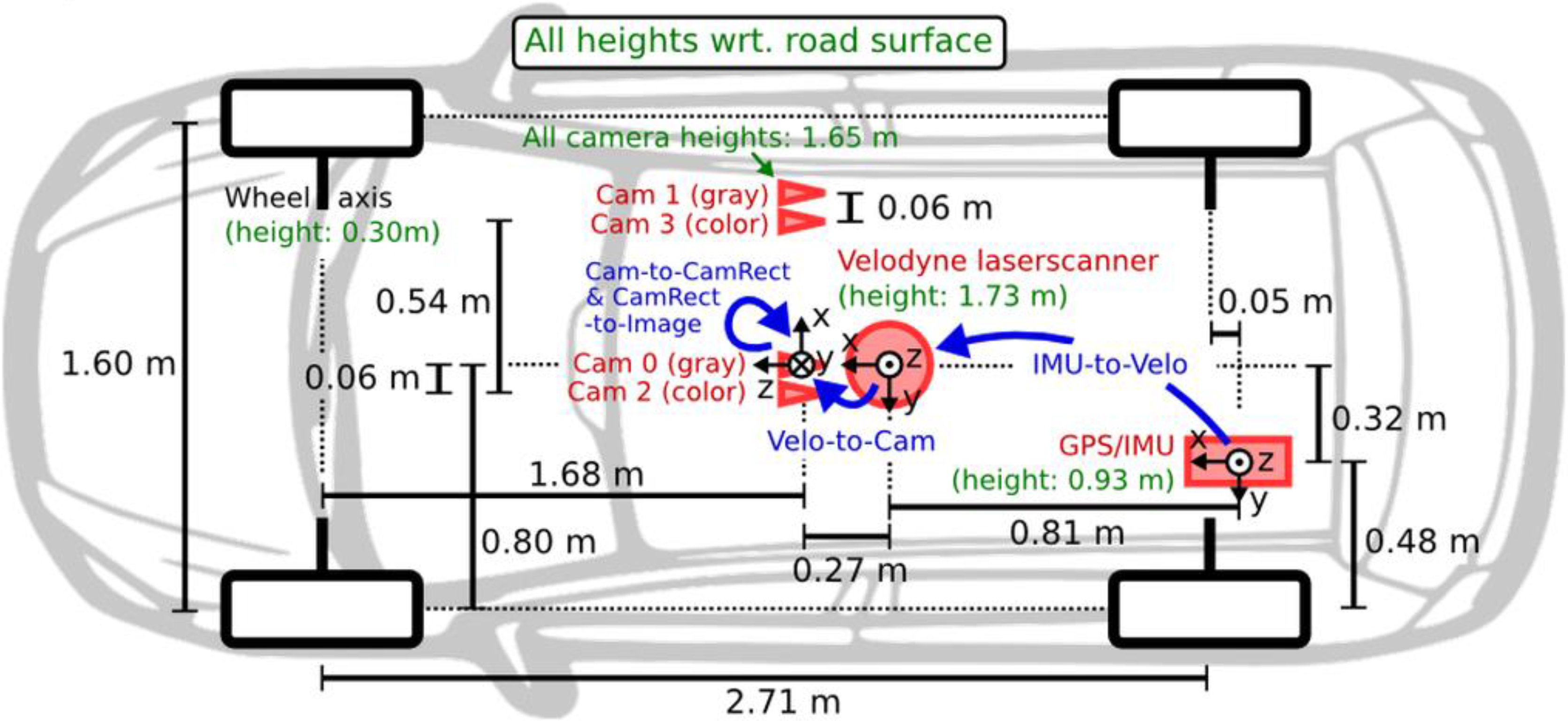
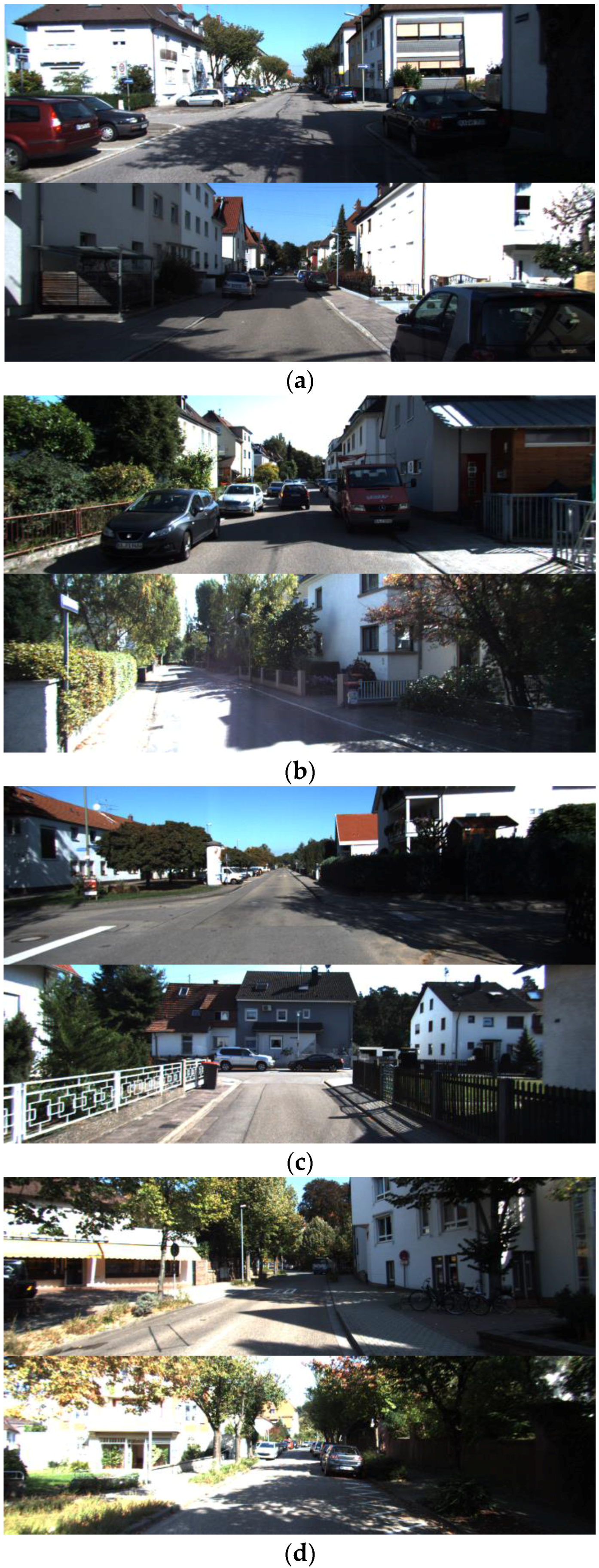
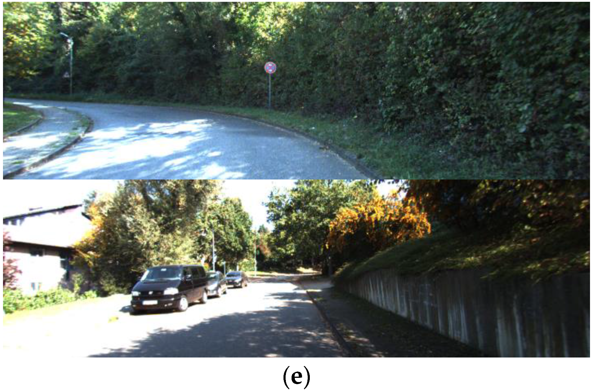
4.1. Data Description

A dataset from KITTI (Karlsruhe Institute of Technology and Toyota technological Institute) is used to assess the integrated system. The sensor data includes monochromic and color image sequences, RTK GPS-IMU data and laser scanner data collected in both urban and suburban areas in City of Karlsruhe, Germany. The used equipments include:

• GPS/IMU: OXTS RT 3003
• Laser scanner: Velodyne HDL-64E
• Grayscale cameras, 1.4 Megapixels: Point Grey Flea 2 (FL2-14S3M-C)
• Color cameras, 1.4 Megapixels: Point Grey Flea 2 (FL2-14S3C-C)

The camera resolution is 1241 × 376 and the data rate is 10 FPS (Frame Per Second). We used gray scale stereo vision for VO, and we used integrated RTK GPS/IMU solution as the ground truth. The sensor configuration is shown in Figure 3.

Figure 3. The sensor configuration on the platform [28].

Figure 3. The sensor configuration on the platform [28].

The dataset #27 collected on 3 October 2011 and the dataset #28 and #18 collected on 30 September 2011 and the dataset # 61 collected on 26 September 2011 and the dataset #34 collected on 3 October 2011 are used to evaluate the pose estimation results.

4.2. Sensor Calibration

All KITTI sensors were carefully synchronized and calibrated [28]. To avoid drift over time, sensors were calibrated every day after KITTI group data collection. In order to synchronize the sensors, Velodyne timestamps were used. KITTI group mounted a reed contact at the bottom of Velodyne, triggering the cameras when facing forward [28]. Unfortunately, a GPS/IMU system cannot be synchronized that way. GPS/IMU provides updates at 100 Hz and the closest timestamp to Velodyne timestamp was selected at each epoch. This synchronization results in maximum 5 ms between GPS/IMU and camera/Velodyne data package. Camera to camera calibration parameters were estimated by the approach proposed in [29]. For camera to camera calibration, a planer chessboard pattern were used. Instead of capturing multiple images of a single chessboard, a single shot of multiple chessboards were taken to estimate intrinsic and extrinsic camera calibration parameters [29]. The estimated intrinsic calibration parameters include left and right camera matrix:

$$(M_i=\left(\begin{array}{ccc}{f}^{\left(i\right)}& 0& c_x^{\left(i\right)}\\ 0& f^{\left(i\right)}& c_y^{\left(i\right)}\\ 0& 0& 0\end{array}\right) i=1,2$$

where f is focal length and C_x and C_y are coordinate of principle center) and image distortion coefficients. The extrinsic camera calibration parameters are rotation and translation between left and right camera coordinate system, essential matrix and fundamental matrix [30,31]. KITTI images were stereo rectified and rectification transform and projection matrix for left and right camera were estimated. The accuracy of camera calibration has a great influence on triangulation and resectioning in VO and inaccurate camera calibration results in faster position drifts in VO. The quality of the stereo camera calibration can be checked by using epipolar geometry constraint [10,30]. The corresponding pixel of a pixel in the left image lies on epiline in the right image. This epiline can be expressed by following Equation (10):

$$l^{\prime }=Fx$$

(18)

where $l^{\prime }$ is epiline in the right image, x is the inhomogeneous pixel coordinate in the left image and F is a 3 × 3 matrix known as a fundamental matrix.

The corresponding pixel in the right image ($x^{\prime }$) lies on the epiline in the right image and therefore:

$$x^{\prime T} l^{\prime }=x^{\prime T}Fx=0$$

(19)

The fundamental matrix, which is one of the outputs of stereo camera calibration, can be used in Equation (19) to assess the quality of stereo camera calibration. The average camera reprojection error for KITTI datasets is 0.3 pixels (The reprojection error less than one pixel is acceptable).

The transformation between the IMU and Velodyne coordinate system and Velodyne and camera coordinate system were estimated by the approach proposed in [29] as well. As we mentioned above, Generalized Iterative Closest Point (GICP) uses stereo VO outputs as initial guess; therefore, the GICP results depend on the accuracy of transformation between Velodyne and a camera coordinate system. The accuracy of the transformation between IMU and Velodyne is important for integration of stereo visual- Lidar and reduced IMU as well. The Velodyne HDL-64E accuracy is +/−2 cm; therefore, the lever arm accuracy which is on the millimeter level accuracy does not affect the system performance.

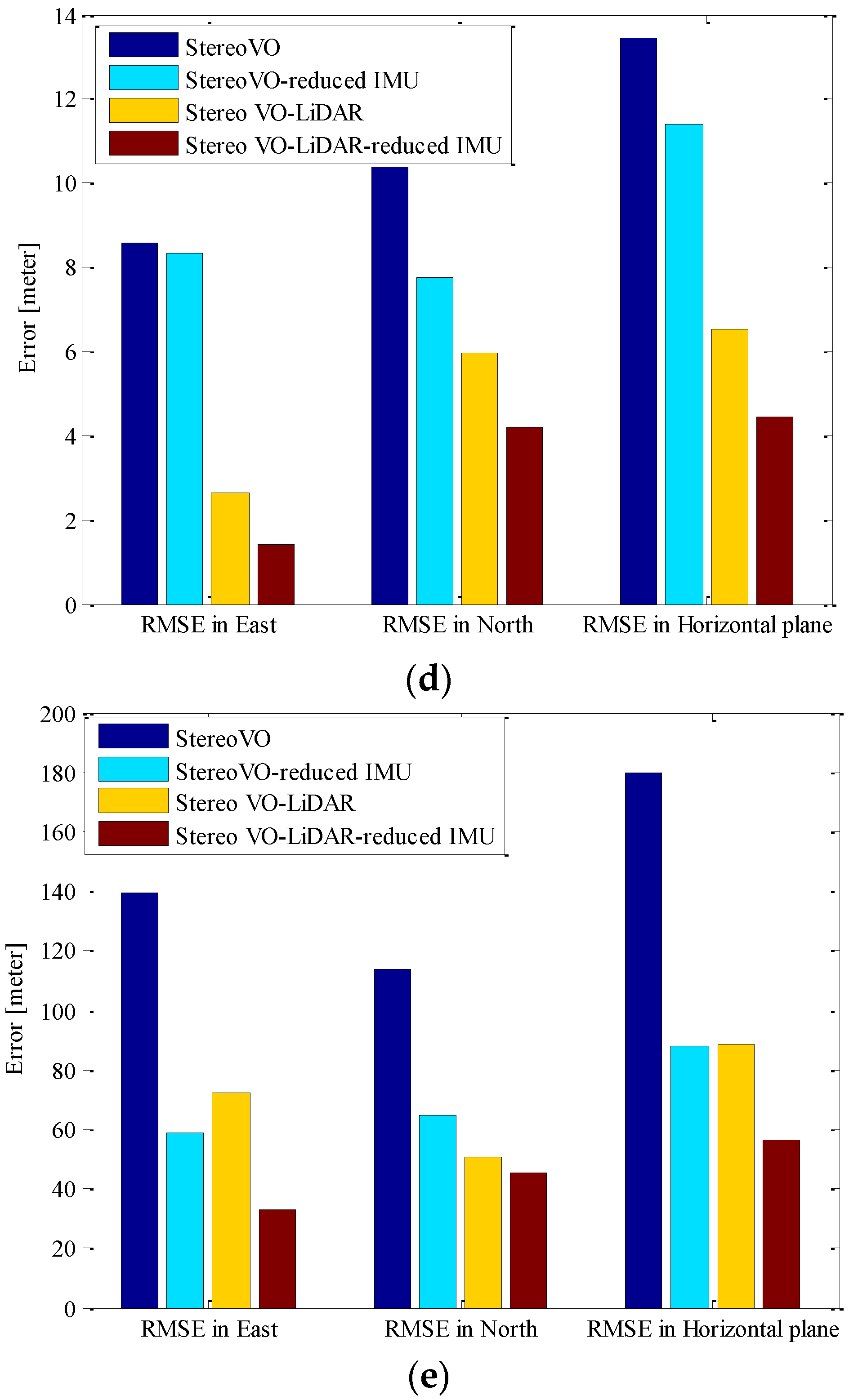
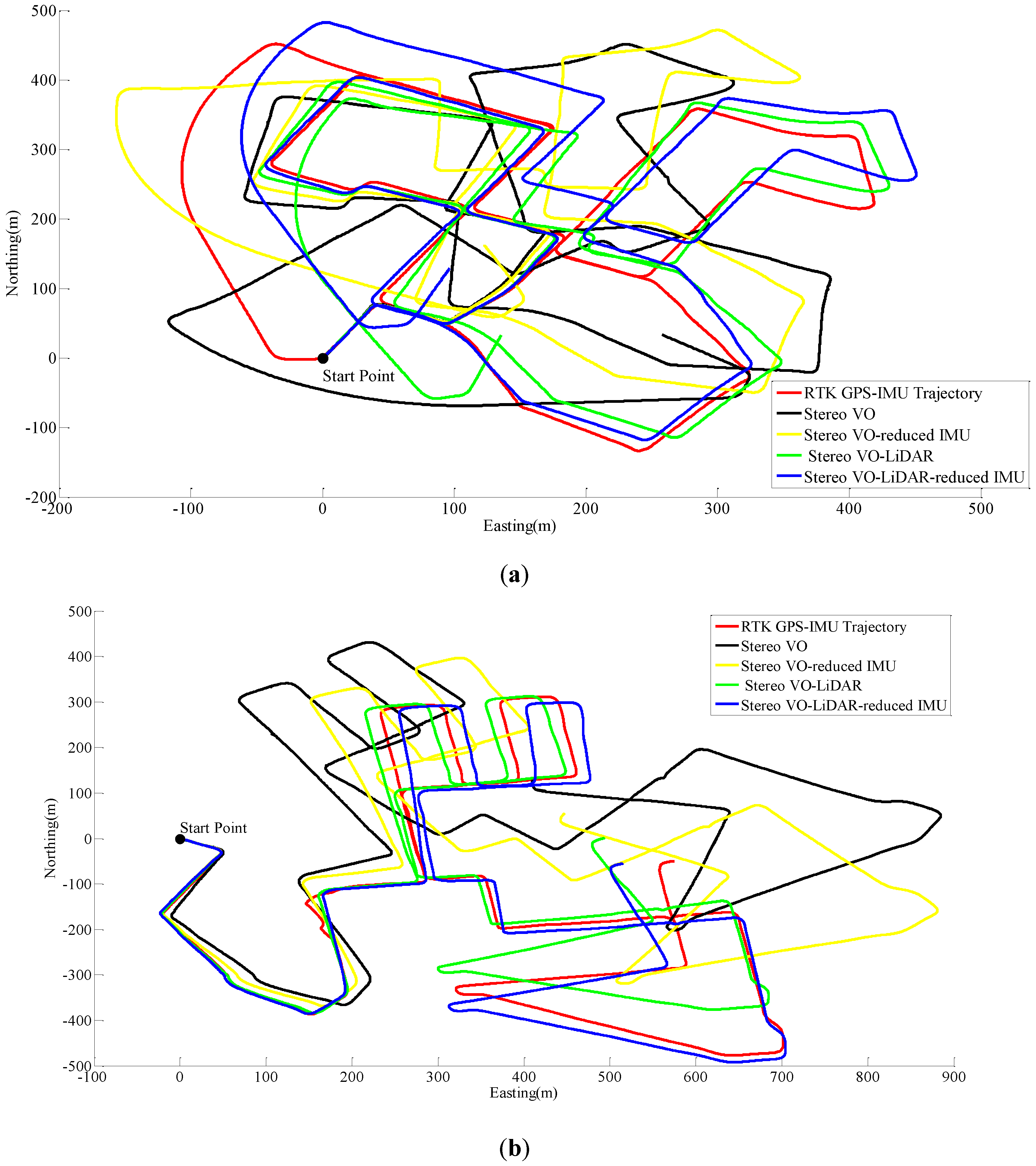
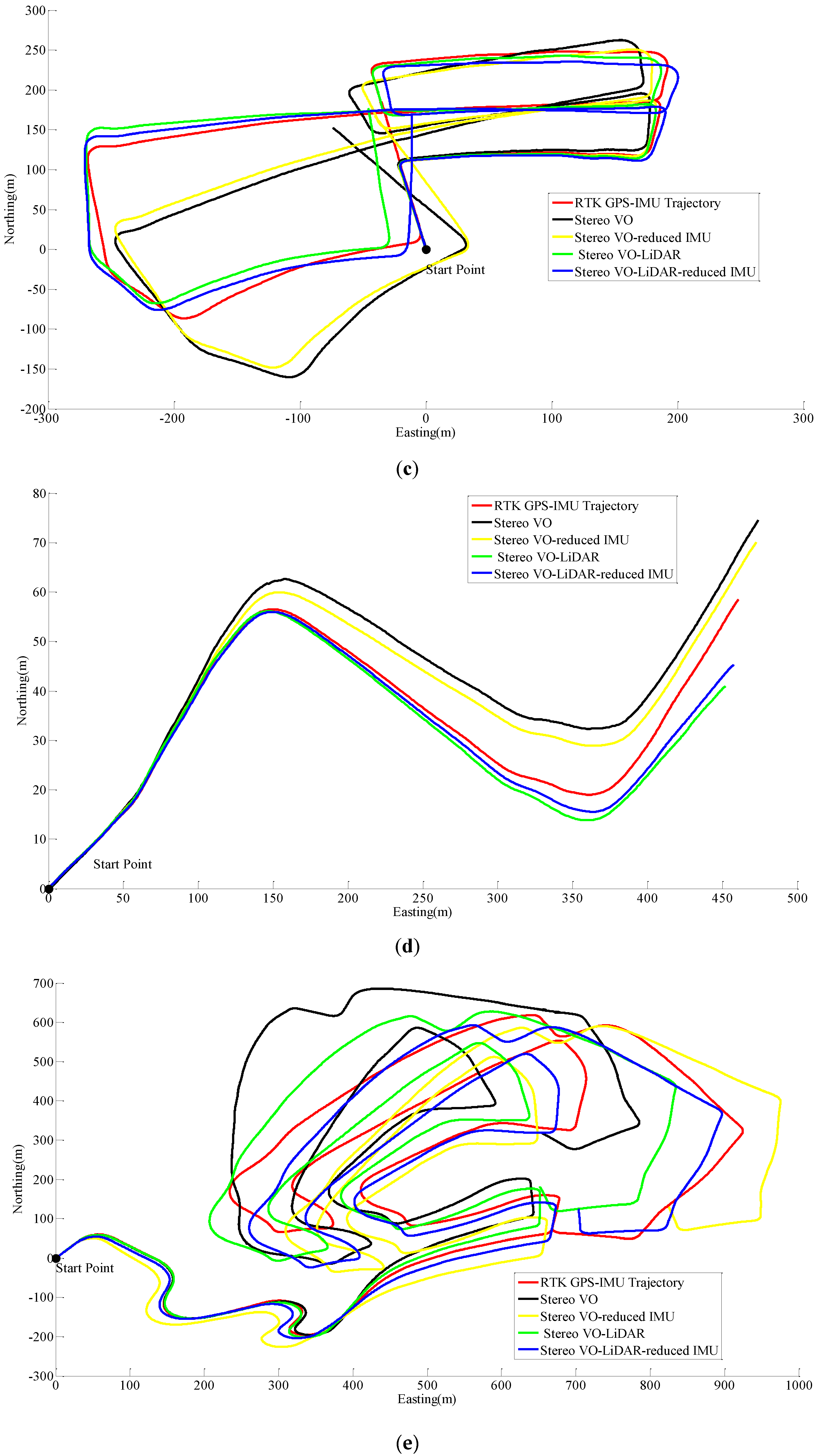
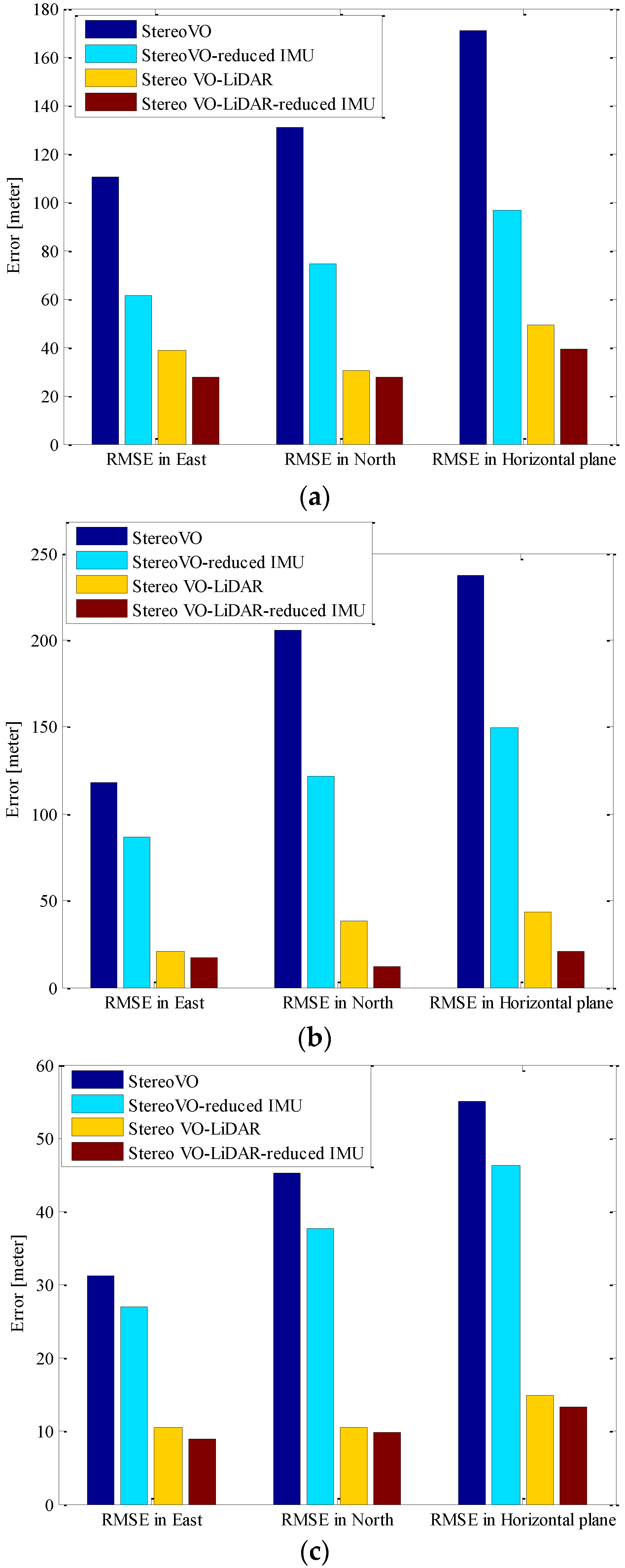
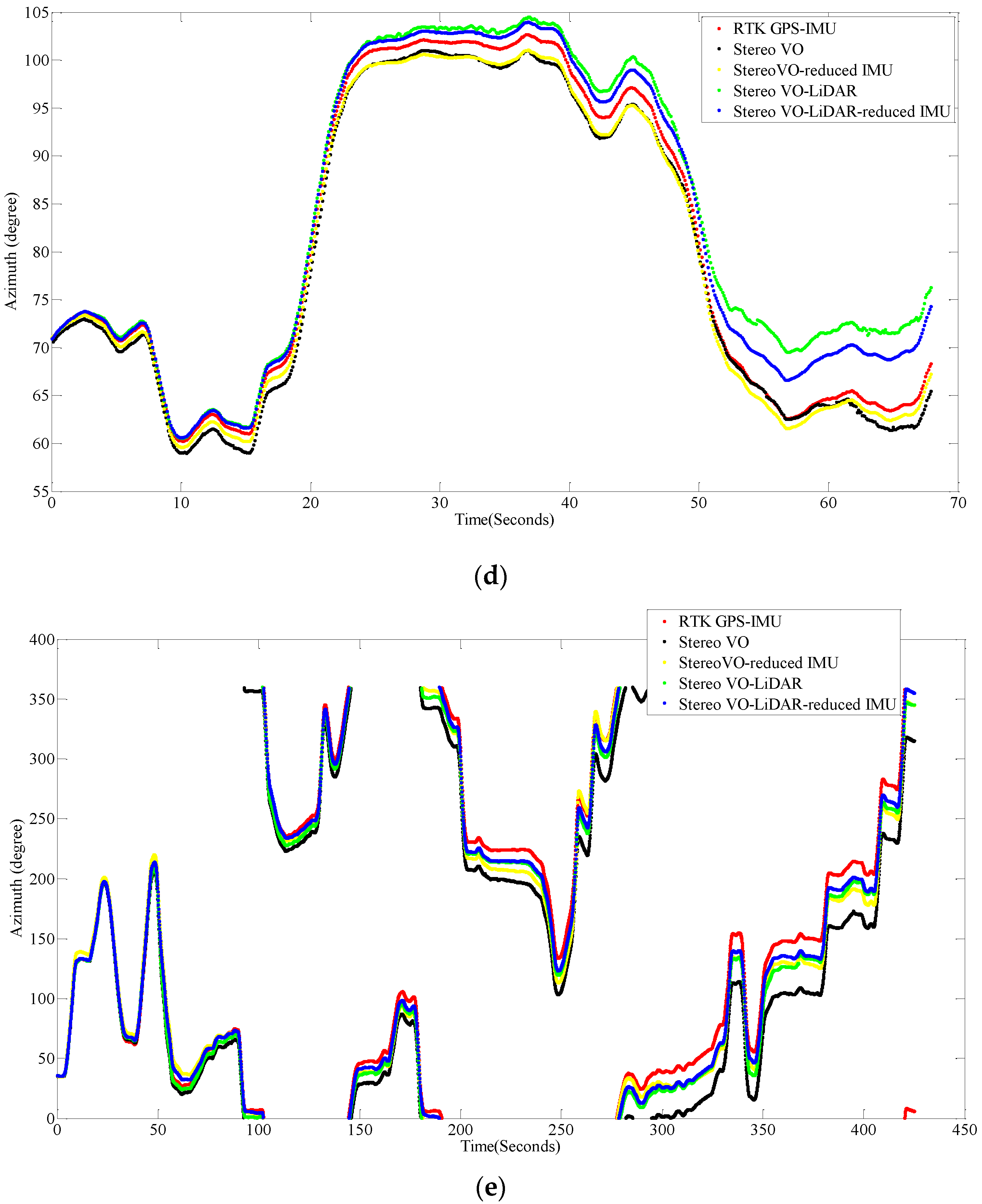
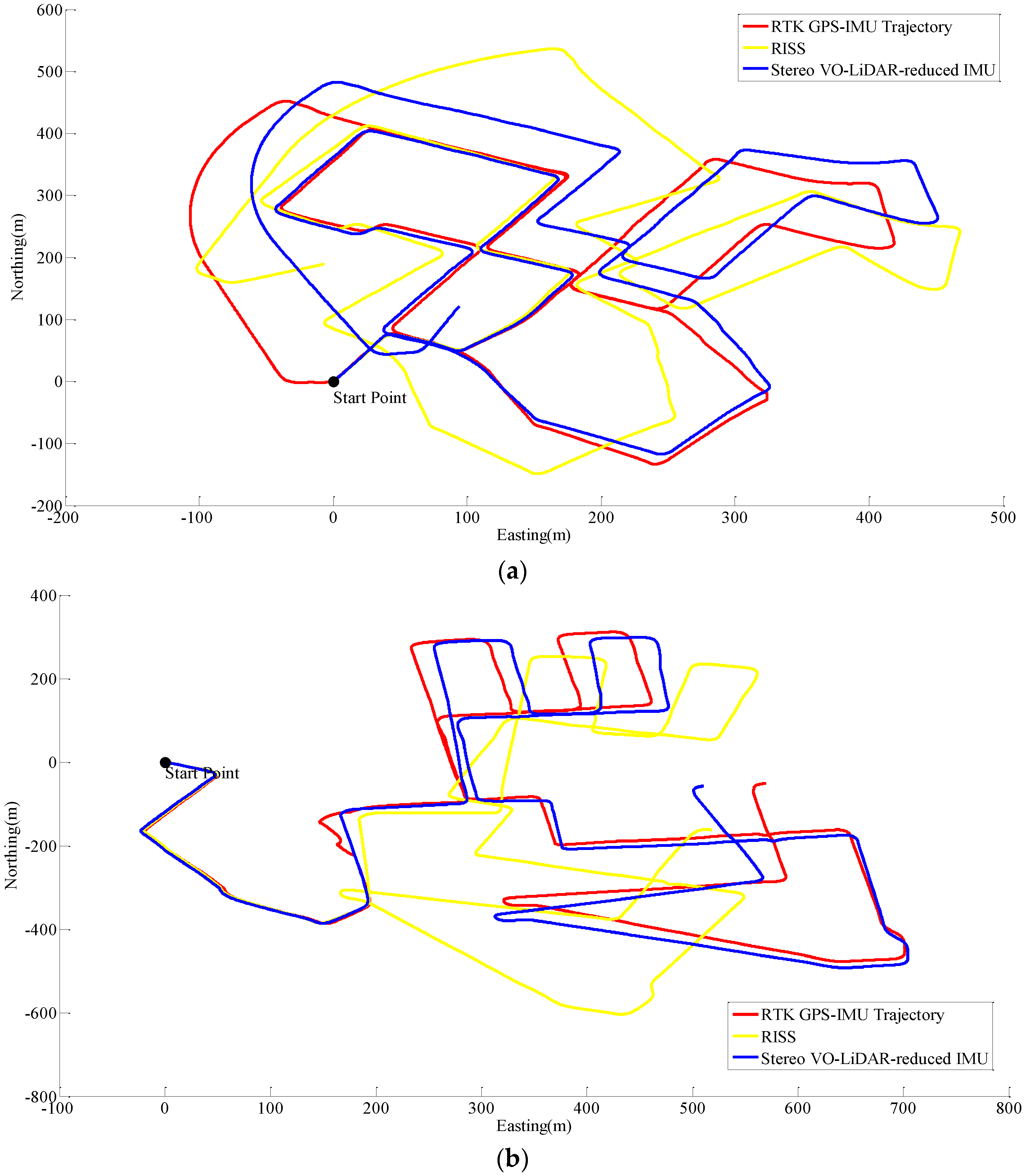
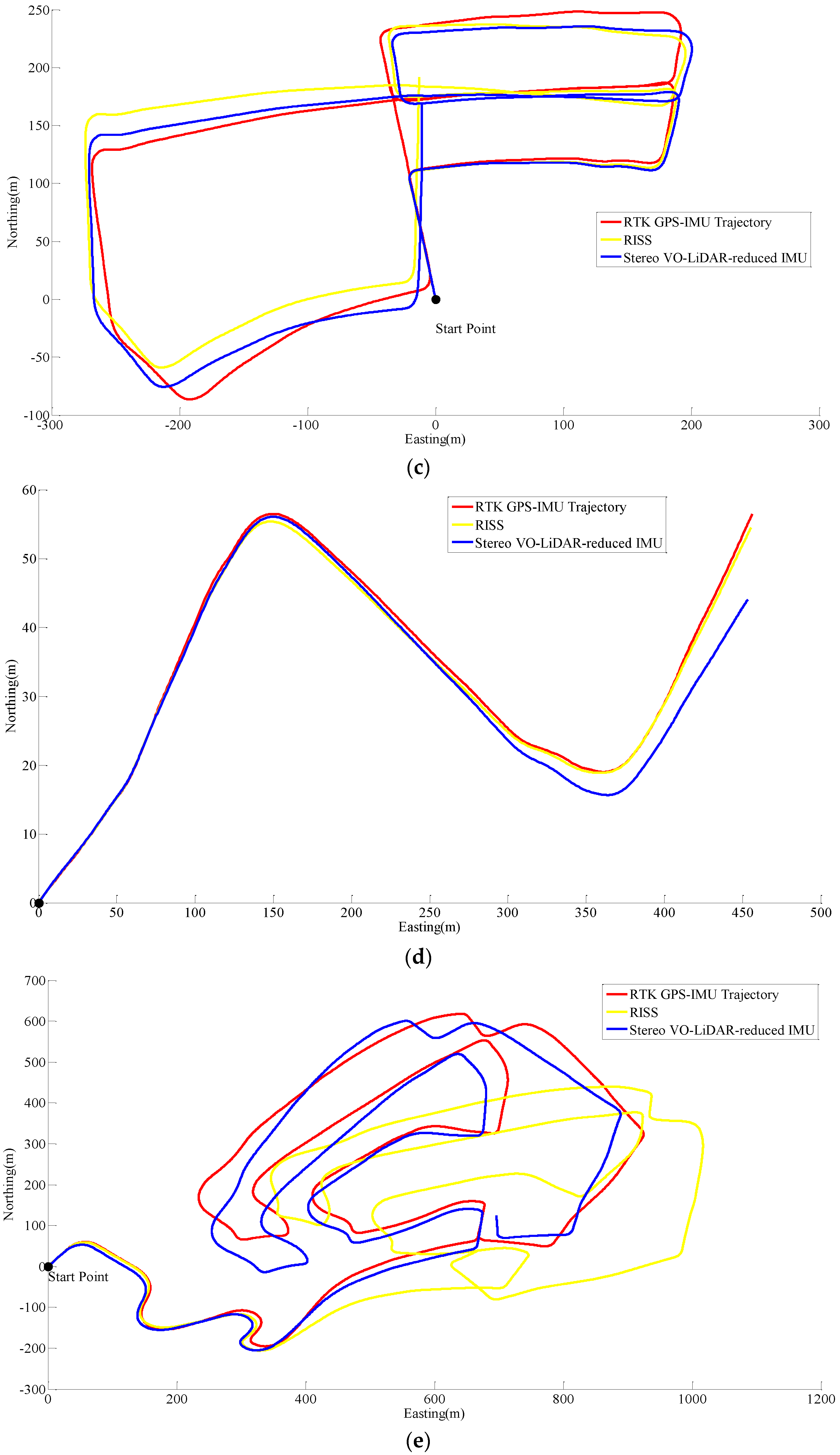
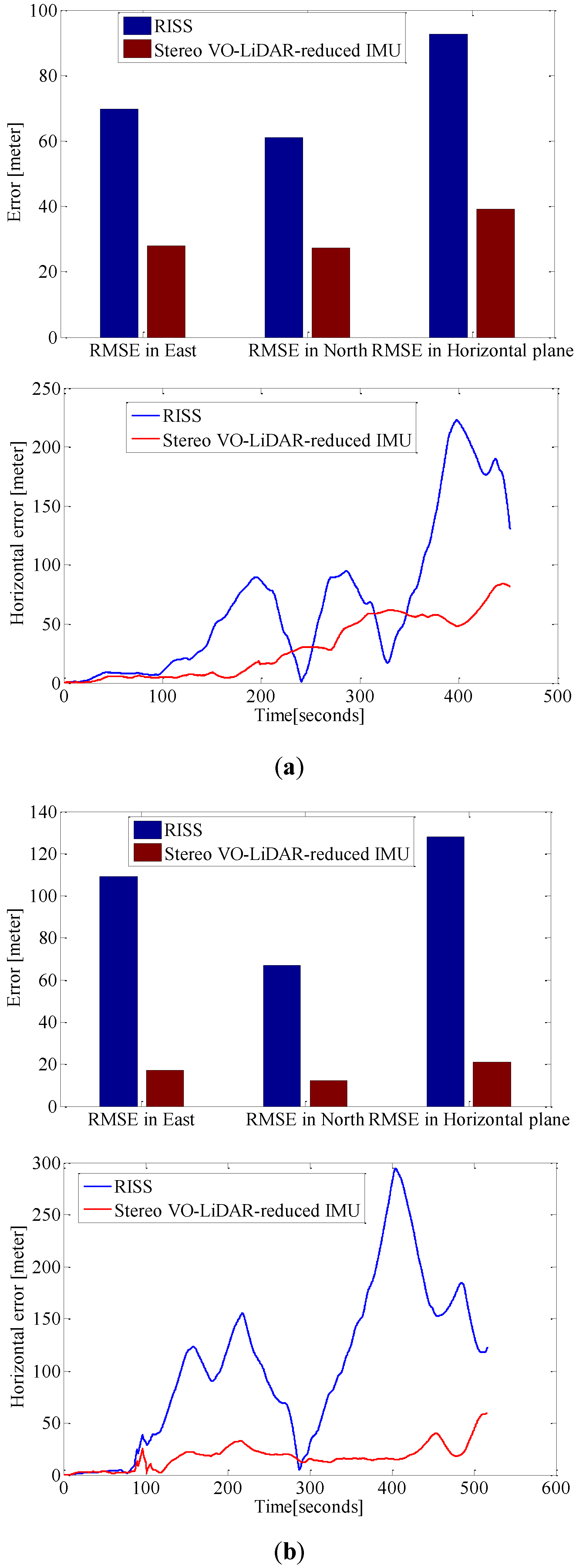
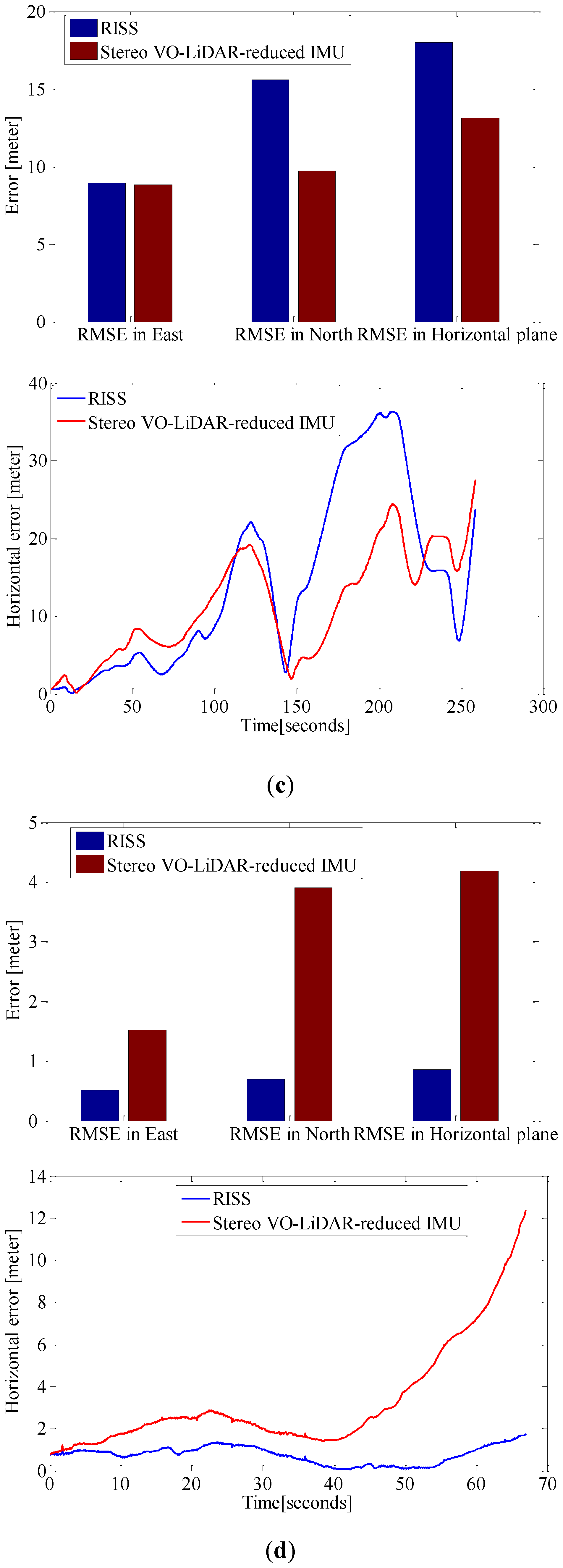
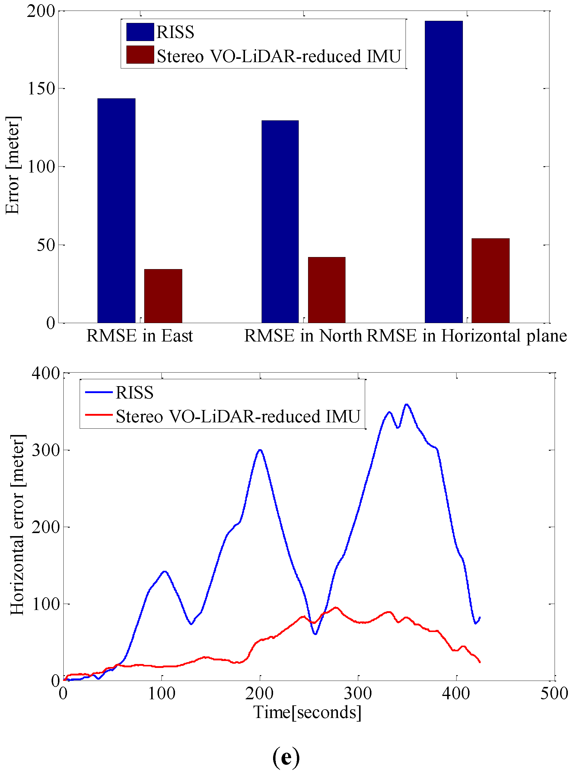
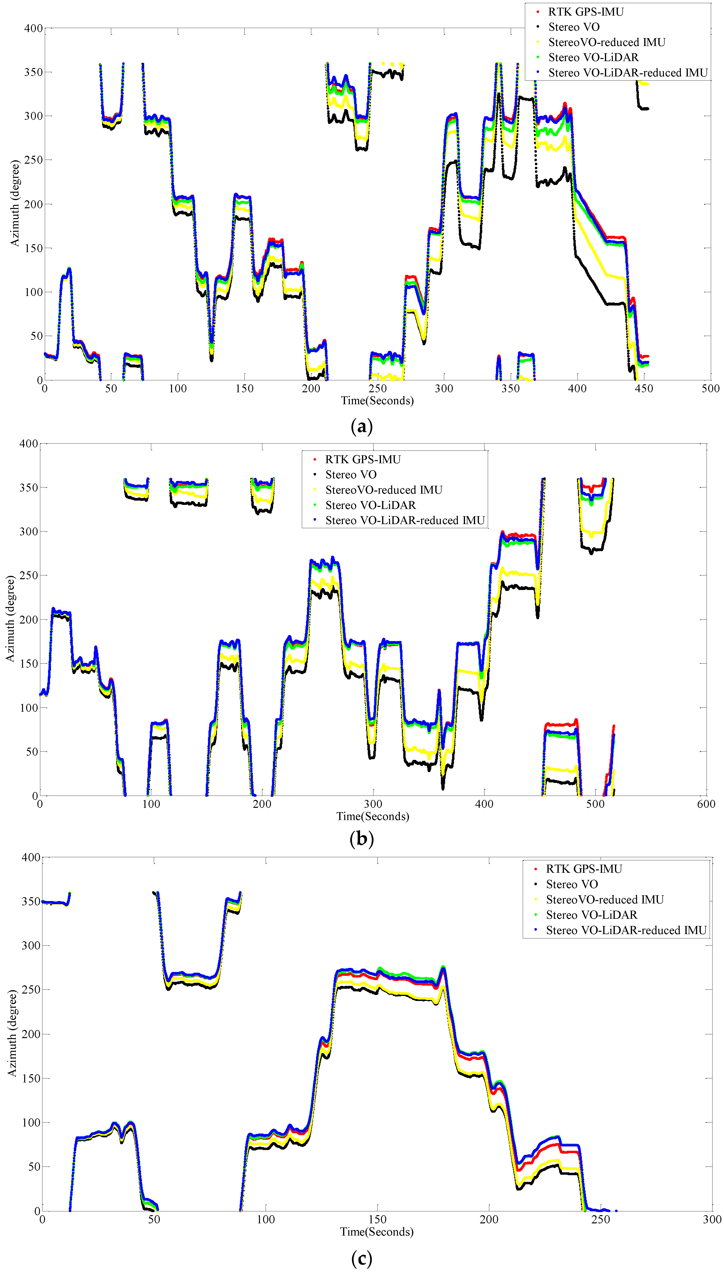
4.3. Sensor Integration Results and Analysis

As we mentioned above, five datasets were used to evaluate and compare the following system configurations in both urban and suburban areas: (1) the stereo VO; (2) the integrated stereo VO and reduced IMU; (3) the Stereo VO-LiDAR; and (4) integrated Stereo VO-LiDAR and reduced IMU.

Figure 4 shows images taken at two epochs of dataset #27, dataset #28, dataset #18, dataset #61 and dataset #34.

Figure 4. (a) shows images at two epochs for dataset #27; (b) for dataset #28; (c) for dataset #18; (d) for dataset #61 and (e) for dataset #34.

Figure 4. (a) shows images at two epochs for dataset #27; (b) for dataset #28; (c) for dataset #18; (d) for dataset #61 and (e) for dataset #34.

Figure 5 shows the pose estimation results for dataset #27, dataset #28, dataset #18, dataset #61 and dataset #34.

Figure 5. Results of ego estimation using stereo VO, integrated stereo VO and reduced IMU, Stereo VO-LiDAR and integrated Stereo VO-LiDAR and reduced IMU. (a) shows results for dataset #27; (b) shows results for dataset #28; (c) shows results for dataset #18; (d) shows results for dataset #61 and (e) shows results for dataset #34.

Figure 5. Results of ego estimation using stereo VO, integrated stereo VO and reduced IMU, Stereo VO-LiDAR and integrated Stereo VO-LiDAR and reduced IMU. (a) shows results for dataset #27; (b) shows results for dataset #28; (c) shows results for dataset #18; (d) shows results for dataset #61 and (e) shows results for dataset #34.

Figure 6 shows the RMSE (Root Mean Square Error) in the east, north and horizontal plane for stereo VO, integrated stereo VO and reduced IMU, Stereo VO-LiDAR and integrated Stereo VO-LiDAR and reduced IMU. Figure 6a show the results for dataset #27, Figure 6b for dataset #28, Figure 6c for dataset #18, Figure 6d for dataset #61 and Figure 6e for dataset #34.

Figure 6. RMSE in east, north and horizontal plane for stereo VO, integrated stereo VO and reduced IMU, Stereo VO-LiDAR and integrated Stereo VO-LiDAR and reduced IMU. (a) shows results for dataset #27; (b) shows results for dataset #28; (c) shows results for dataset #18; (d) shows results for dataset #61 and (e) shows results for dataset #34.

Figure 6. RMSE in east, north and horizontal plane for stereo VO, integrated stereo VO and reduced IMU, Stereo VO-LiDAR and integrated Stereo VO-LiDAR and reduced IMU. (a) shows results for dataset #27; (b) shows results for dataset #28; (c) shows results for dataset #18; (d) shows results for dataset #61 and (e) shows results for dataset #34.

The measured drifts are compared to the distance traveled as the relative accuracy and listed in Table 1.

Table 1. Relative horizontal position errors in filed test. VO: Stereo Visual Odometry, VO-RI: Integrated Stereo Visual Odometry and Reduced IMU, VO-L: Stereo Visual-LiDAR Odometry, VO-L-RI: Integrated. Stereo Visual-LiDAR Odometry and Reduced IMU.

Dataset No.	Dist.	Relative Horizontal Position Error
		VO	VO-RI	VO-L	VO-L-RI
dataset #27	3705 m	4.62%	2.60%	1.33%	1.05%
dataset #28	4110 m	5.77%	3.64%	1.06%	0.51%
dataset #18	2025 m	2.71%	2.29%	0.73%	0.65%
dataset #61	485 m	2.78%	2.34%	1.34%	0.91%
dataset #34	4509 m	3.99%	1.94%	1.96%	1.25%

Table 1. Relative horizontal position errors in filed test. VO: Stereo Visual Odometry, VO-RI: Integrated Stereo Visual Odometry and Reduced IMU, VO-L: Stereo Visual-LiDAR Odometry, VO-L-RI: Integrated. Stereo Visual-LiDAR Odometry and Reduced IMU.

Dataset No.	Dist.	Relative Horizontal Position Error
		VO	VO-RI	VO-L	VO-L-RI
dataset #27	3705 m	4.62%	2.60%	1.33%	1.05%
dataset #28	4110 m	5.77%	3.64%	1.06%	0.51%
dataset #18	2025 m	2.71%	2.29%	0.73%	0.65%
dataset #61	485 m	2.78%	2.34%	1.34%	0.91%
dataset #34	4509 m	3.99%	1.94%	1.96%	1.25%

Figure 7 shows the vehicle azimuth for dataset #27, dataset #28, dataset #18, dataset #61 and dataset #34.

Figure 7. Vehicle azimuth calculated by VO, VO-RI, VO-L and VO-L-RI, (a) for dataset #27; (b) for dataset #28; (c) for dataset #18; (d) for dataset #61 and (e) for dataset #34.

Figure 7. Vehicle azimuth calculated by VO, VO-RI, VO-L and VO-L-RI, (a) for dataset #27; (b) for dataset #28; (c) for dataset #18; (d) for dataset #61 and (e) for dataset #34.

As we can see from the above results, the integrated stereo Visual-LiDAR odometry and 3D reduced IMU gives more accurate results than the other methods. For all data sets, this method drifts more slowly and gives better results than other methods. The stereo visual-LiDAR odometry gives better results than the stand alone stereo VO and the integrated stereo VO and reduced IMU for the first four datasets which were collected in urban areas with buildings around. For dataset # 34, it is slightly worse than the integrated stereo VO and reduced IMU, because this dataset was collected in small roads with vegetations in the scene. The LiDAR odometry gives poorer results in suburban areas, and it might fail if the point clouds are very sparse without any specific shape. Furthermore, the integrated stereo Visual-LiDAR odometry and 3D reduced IMU azimuth is more accurate than other methods. The integrated stereo visual-LiDAR odometry and reduced IMU can achieve accuracy at the level of state of art results proposed by [4]. Zhang et al. [4] proposed a visual-LiDAR odometry and mapping method with an average of 0.75% of relative position drift. Our method has an average of 0.78% of relative position drift in urban areas. Zhang et al. [4] uses monocular camera for VO and uses LiDAR to remove the camera scale ambiguity; in other words, their method tightly couples monocular camera and LiDAR. Afterwards, they used the output of monocular camera and LiDAR as the input of ICP in order to refine pose estimation. In this paper, a stereo camera was used to remove scale ambiguity, and it does not depend on other sensors. LiDAR uses stereo VO outputs as the initial guess for ICP and if stereo VO fails, LiDAR odometry can still work (we can use point cloud registration methods to provide initial guess for ICP). Tightly coupled monocular camera and LIDAR is more accurate than stereo VO. Therefore, the initial guess for ICP in [4] is better than our initial guess. Therefore, vision-LiDAR block in [4] performs better than vision-LiDAR block in our method. On the other hand, our proposed method is more reliable. In [4], if the point clouds are sparse, no depth can be assigned to visual keypoints and there would be no solution for that epoch. In our system, if LiDAR fails, stereo VO can still give us the solution. Finally, we add reduced IMU to our system to reach similar accuracy as [4].

Unfortunately, online KITTI datasets did not include wheel odometer data; therefore, the wheel odometer data in RISS, is replaced by RTK GPS/IMU forward velocity in order to compare simulated RISS and proposed method. RTK GPS/IMU forward velocity is more accurate than wheel odometer which suffers from many factors such as tyre slippage and tyre diameter variation due to the speed and pressure changes [31]. Figure 8 shows RISS and integrated stereo VO-LIDAR and reduced IMU pose estimation results for dataset #27, dataset #28, dataset #18, dataset #61 and dataset #34.

Figure 8. Results of ego estimation using RISS and integrated Stereo VO-LiDAR and reduced IMU. (a) shows results for dataset #27; (b) shows results for dataset #28; (c) shows results for dataset #18; (d) shows results for dataset #61 and (e) shows results for dataset #34.

Figure 8. Results of ego estimation using RISS and integrated Stereo VO-LiDAR and reduced IMU. (a) shows results for dataset #27; (b) shows results for dataset #28; (c) shows results for dataset #18; (d) shows results for dataset #61 and (e) shows results for dataset #34.

Figure 9 shows the RMSE in the east, north and horizontal plane and horizontal error of estimated positions for RISS and integrated Stereo VO-LiDAR and reduced IMU. Figure 9a show the results for dataset #27, Figure 9b for dataset #28, Figute 9c for dataset #18, Figure 9d for dataset #61 and Figure 9e for dataset #34.

Figure 9. RMSE in east, north and horizontal plane for RISS and integrated Stereo VO-LiDAR and reduced IMU. (a) shows results for dataset #27; (b) shows results for dataset #28; (c) shows results for dataset #18; (d) shows results for dataset #61 and (e) shows results for dataset #34.

Figure 9. RMSE in east, north and horizontal plane for RISS and integrated Stereo VO-LiDAR and reduced IMU. (a) shows results for dataset #27; (b) shows results for dataset #28; (c) shows results for dataset #18; (d) shows results for dataset #61 and (e) shows results for dataset #34.

Although RTK GPS/IMU forward velocity is more accurate than wheel odometer as well as stereo VO-LiDAR velocity, integrated stereo VO-LiDAR and reduced IMU outperforms simulated RISS for all datasets except dataset # 61. In RISS, vertical gyro output, roll, pitch and forward velocity are used to calculate the azimuth. RISS azimuth is accurate for short time and the azimuth accuracy degrades fast due to gyro error accumulation. As we mentioned in the introduction part, stereo VO-LiDAR provides both velocity and azimuth. Stereo VO-LiDAR azimuth is integrated with vertical gyro azimuth in the proposed method resulting in more accurate and stable results. Simulated RISS results is better than proposed method for dataset #61, because this dataset is very short (67 s only) and data ends before vertcal gyro azimuth starts to deviate.

5. Conclusions

An integrated stereo visual-LiDAR odometry and reduced IMU is proposed in this paper in which first the stereo visual odometer estimates ego motion which is used to register point clouds then the GICP algorithm is used to refine the ego motion estimation, and, finally, the forward velocity and azimuth obtained by a visual-LiDAR odometer are integrated with reduced IMU in an Extended Kalman Filter (EKF) to provide final navigation solution. The proposed system outperforms the simulated Reduced Inertial Sensor System (RISS). A stereo visual-LiDAR odometer provides not only the translation but also the rotation between two laser scanner coordinate systems at consecutive epochs. Therefore, we can calculate VO-LiDAR azimuth at each epoch which will be integrated with the reduced IMU azimuth. The results show that the integrated stereo visual-LiDAR odometry and 3D reduced IMU gives more accurate results than the stereo VO, the integrated stereo VO and reduced IMU, and the stereo visual-LiDAR odometry. The stereo visual-LiDAR odomery is slightly worse than the integrated stereo VO and reduced IMU in suburban areas (small roads with vegetations in the scene). The results also indicate that the integrated stereo visual-LiDAR odometry and reduced IMU can achieve accuracy at the level comparable to the state-of-the-art. KITTI datasets do not include wheel odometer data. To simulate RISS, the wheel odometer data was replaced by RTK GPS/IMU forward velocity, which is more accurate than the wheel odometer. Integrated stereo VO-LIDAR and reduced IMU outperforms simulated RISS for all datasets except dataset # 61. Dataset # 61 is very short and data ends before vertical gyro azimuth starts to deviate.

6. Future Work

Extensive research has been done in odometry side slip estimation and compensation using a standard IMU. In this paper, the KITTI datasets do not include specific data for side slip estimation, and we will consider it as a future task.

References

1. Milella, A.; Siegwart, R. Stereo-based ego-motion estimation using pixel tracking and iterative closest point. In Proceedings of the IEEE International Conference on Computer Vision Systems, New York, NY, USA, 4–7 January 2006; p. 21.
2. Hong, S.; Ko, H.; Kim, J. VICP: Velocity updating iterative closest point algorithm. In Proceedings of the 2010 IEEE International Conference on Robotics and Automation, Anchorage, AK, USA, 3–7 May 2010; pp. 1893–1898.
3. Hong, S.; Ko, H.; Kim, J. Improved motion tracking with velocity update and distortion correction from planar laser scan data. In Proceedings of the International Conference Artificial Reality and Telexistence, 1–3 December 2008; pp. 315–318.
4. Zhang, J.; Singh, S. Visual-lidar odometry and mapping: Low-drift, robust, and fast. In Proceedings of the 2015 IEEE International Conference on Robotics and Automation (ICRA), Seattle, WA, USA, 26–30 May 2015; pp. 2174–2181.
5. Noureldin, A.; Karamat, T.B.; Georgy, J. Fundamentals of Inertial Navigation, Satellite-Based Positioning and Their Integration; Springer: Berlin, Germany, 2013. [Google Scholar]
6. Kitt, B.; Geiger, A.; Lategahn, H. Visual odometry based on stereo image sequences with RANSAC-based outlier rejection scheme. In Proceedings of the 2010 IEEE Intelligent Vehicles Symposium, San Diego, CA, USA, 21–24 June 2010; pp. 486–492.
7. Scaramuzza, D.; Fraundorfer, F. Tutorial: Visual odometry. IEEE Robot. Autom. Mag. 2011, 18, 80–92. [Google Scholar] [CrossRef]
8. Steffen, R. Visual SLAM from Image Sequences Acquired by Unmanned Aerial Vehicles. Ph.D. Thesis, University of Bonn, Bonn, Germany, 2009. [Google Scholar]
9. Weiss, S. Visual SLAM in Pieces; ETH Zurich: Zurich, Switzerland, 2009. [Google Scholar]
10. Hosseinyalamdary, S.; Yilmaz, A. Motion vector field estimation using brightness constancy assumption and epipolar geometry constraint. ISPRS Ann. Photogramm. Remote Sens. Spat. Inf. Sci. 2014, II–1, 9–16. [Google Scholar] [CrossRef]
11. Sarvrood, Y.B.; Gao, Y. Analysis and reduction of stereo vision alignment and velocity errors for vision navigation. In Proceedings of the 27th International Technical Meeting of The Satellite Division of the Institute of Navigation, San Diego, CA, USA, 27–29 January 2014; pp. 3254–3262.
12. Holz, D.; Ichim, A.E.; Tombari, F.; Rusu, R.B.; Behnke, S. Registration with the point cloud library PCL A modular framework for aligning 3D point clouds. IEEE Robot. Autom. Mag. 2015, 22, 110–124. [Google Scholar] [CrossRef]
13. Biber, P.; Strasser, W. The normal distributions transform: A new approach to laser scan matching. IEEE Int. Conf. Intell. Robot. Syst. 2003, 3, 2743–2748. [Google Scholar]
14. Low, K. Linear Least-Squares Optimization for Point-to-Plane ICP Surface Registration; The University of North Carolina at Chapel Hill: Chapel Hill, NC, USA, 2004. [Google Scholar]
15. Segal, A.; Haehnel, D.; Thrun, S. Generalized-ICP. Robot. Sci. Syst. 2009, 5, 168–176. [Google Scholar]
16. Sirtkaya, S.; Seymen, B.; Alatan, A. Loosely coupled Kalman filtering for fusion of Visual Odometry and inertial navigation. In Proceedings of the 2013 16th International Conference on Information Fusion (FUSION), Istanbul, Turkey, 9–12 July 2013; pp. 219–226.
17. Corke, P.; Lobo, J.; Dias, J. An introduction to inertial and visual sensing. Int. J. Rob. Res. 2007, 26, 519–535. [Google Scholar] [CrossRef]
18. Qian, G.; Chellappa, R.; Zheng, Q. Robust structure from motion estimation using inertial data. J. Opt. Soc. Am. A 2001, 18, 2982. [Google Scholar] [CrossRef]
19. Kleinert, M.; Schleith, S. Inertial aided monocular SLAM for GPS-denied navigation. In Proceedings of the IEEE International Conference on Multisensor Fusion and Integration for Intelligent Systems (MFI), Salt Lake City, UT, USA, 5–7 September 2010; pp. 20–25.
20. Nützi, G.; Weiss, S.; Scaramuzza, D.; Siegwart, R. Fusion of IMU and vision for absolute scale estimation in monocular SLAM. J. Intell. Robot. Syst. Theory Appl. 2011, 61, 287–299. [Google Scholar] [CrossRef]
21. Schmid, K.; Hirschmuller, H. Stereo vision and IMU based real-time ego-motion and depth image computation on a handheld device. In Proceedings of the 2013 IEEE International Conference on Robotics and Automation (ICRA), Karlsruhe, Germany, 6–10 May 2013; pp. 4671–4678.
22. Konolige, K.; Agrawal, M.; Sola, J. Large scale visual odometry for rough terrain. Proc. Int. Symp. Robot. Res. 2007, 2, 1150–1157. [Google Scholar]
23. Tardif, J.P.; George, M.; Laverne, M.; Kelly, A.; Stentz, A. A new approach to vision-aided inertial navigation. In Proceedings of the 2010 IEEE/RSJ International Conference on Intelligent Robots and Systems (IROS), Taipei, Taiwan, 18–22 October 2010; pp. 4161–4168.
24. Strelow, D. Motion estimation from image and inertial measurements. Int. J. Rob. Res. 2004, 23, 1157–1195. [Google Scholar] [CrossRef]
25. Scherer, S.; Rehder, J.; Achar, S.; Cover, H.; Chambers, A.; Nuske, S.; Singh, S. River mapping from a flying robot: State estimation, river detection, and obstacle mapping. Auton. Robots 2012, 33, 189–214. [Google Scholar] [CrossRef]
26. Jekeli, C. Inertial Navigation Systems with Geodetic Applications; DE GRUYTER: Berlin, Germany, 2001. [Google Scholar]
27. Szeliski, R. Computer vision: Algorithms and applications. Computer (Long. Beach. Calif). 2010, 5, 832. [Google Scholar]
28. Geiger, A.; Lenz, P.; Stiller, C.; Urtasun, R. Vision meets robotics: The KITTI dataset. Int. J. Rob. Res. 2013, 32, 1231–1237. [Google Scholar] [CrossRef]
29. Geiger, A.; Moosmann, F.; Car, O.; Schuster, B. Automatic camera and range sensor calibration using a single shot. In Proceedings of the 2012 IEEE International Conference on Robotics and Automation (ICRA), Saint Paul, MN, USA, 14–18 May 2012; pp. 3936–3943.
30. Hosseinyalamdary, S.; Balazadegan, Y.; Toth, C. Tracking 3D moving objects based on GPS/IMU navigation solution, laser scanner point cloud and GIS data. ISPRS Int. J. Geo-Inform. 2015, 4, 1301–1316. [Google Scholar] [CrossRef]
31. Meng, Y. Improved positioning of land vehicle in its using digital map and other accessory information. Ph.D. Thesis, Hong Kong Polytechnic University, Hong Kong, 2006. [Google Scholar]