1. Introduction
Nowadays, increased attention is paid to navigation, which supports path-finding or evacuation operations inside a building. Indoor spaces always contain a large variety of static objects, such as desks, chairs, tables and other furniture. There is often no need to consider the size of a pedestrian for obstacle avoidance. Yet, in specific cases, the pedestrian-related dimension is important. For instance, a user is manipulating a machine and she/he needs to move it with her/him.
Pedestrian-related dimensions are specifically important for facility management and maintenance. For example, a member of the maintenance staff in a factory operates a large vehicle, and she/he needs a route that ensures she/he can pass with the vehicle. Similar situations can be seen in airports. A member of staff transports different goods with a wheeled cart. The goods need to be delivered to distinct ports by avoiding obstacles and passing through some narrow spaces. All of these cases require paths that can consider the total size of pedestrians and their objects.
Research on pedestrian indoor navigation has considered indoor obstacles in the navigation network [
1,
2,
3] and obstacle-avoiding path-finding [
4,
5,
6,
7]. However, it has not discussed the influence of user sizes. In contrast, robot motion planning has always taken into consideration the dimensions of the robot. The Minkowski sum method [
8,
9] has been commonly applied to identify inaccessible areas for a robot.
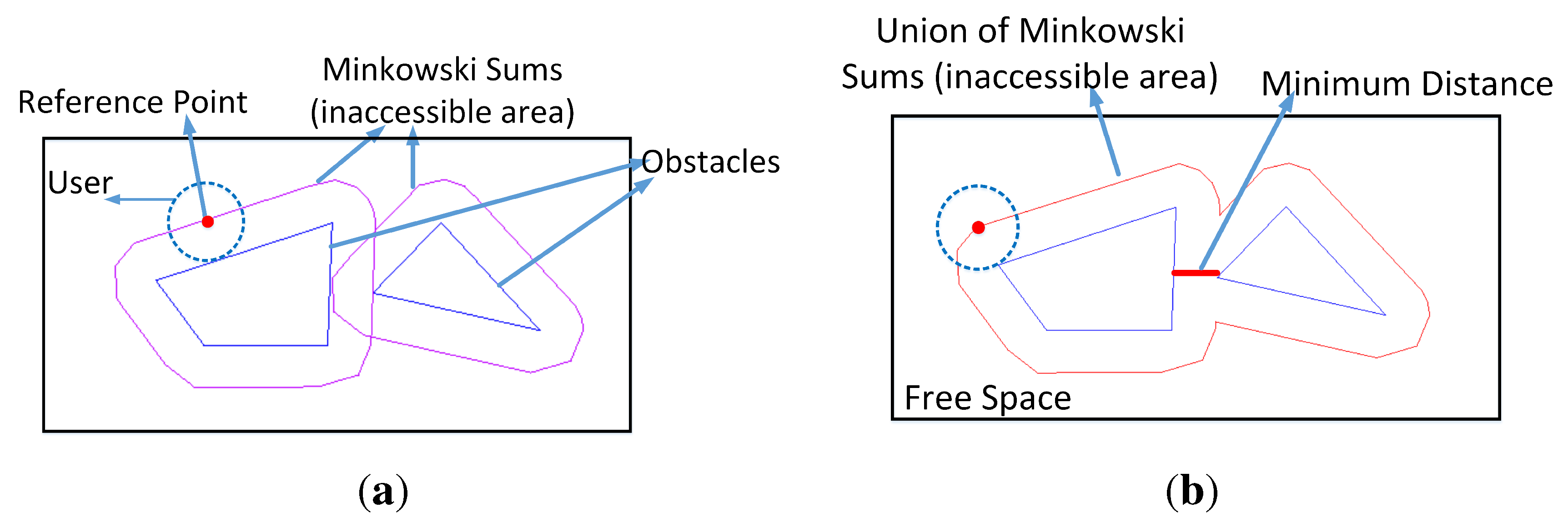
Figure 1 presents an example where a robot is approximated with a circle. A Minkowski sum of an obstacle expands the obstacle according to the robot’s size (the circle’s radius in
Figure 1a), while simultaneously, the robot shrinks to a “reference” point (see
Figure 1a). The Minkowski sum represents the inaccessible area for the robot. If the Minkowski sums of different obstacles intersect, then they will be merged into one to form a closed inaccessible area for the robot (see
Figure 1b). The space outside the union region is regarded as the free space for the robot, and consequently, the robot can follow paths in it.
However, the Minkowski sum approach tends to generate non-simple geometry, because it involves many union operations on polygons. Such a geometry is not convenient for creating a navigation network.
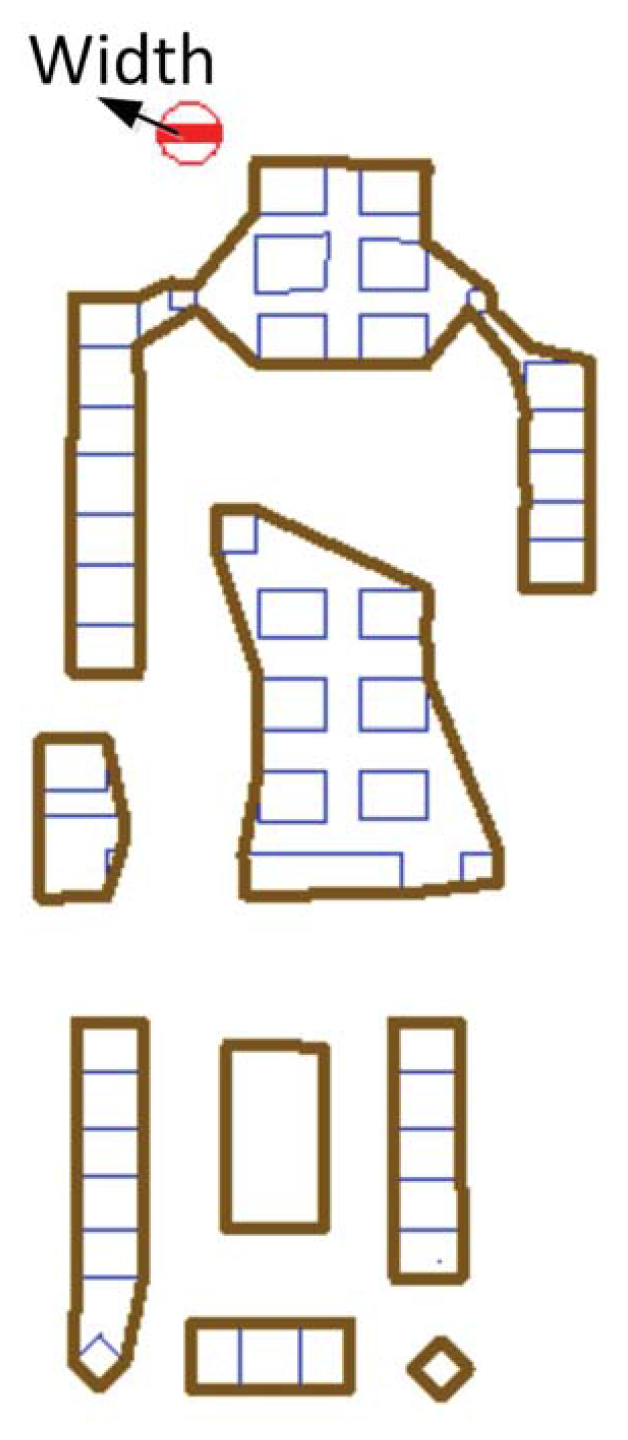
Figure 2 also uses a circle to approximate a pedestrian with related objects/tools.
Figure 2 presents two union results of the Minkowski sums. An isolated inner ring (see
Figure 2a) is part of the merged Minkowski sums of the six objects.
Figure 2b presents the case of self-intersection. Several edges touch each other at the polygon of the merged Minkowski sums, which increases the redundancy of vertices. Furthermore, the generated polygons (see
Figure 2) include too many vertices (e.g., the “curved” parts), which complicates the creation of the network (see below).
Figure 1.
Minkowski sums of obstacles to a user and the minimum distance between obstacles. (a) Minkowski sum of obstacles for a user approximated as a circle; (b) union of the Minkowski sum of obstacles and the minimum distance.
Figure 1.
Minkowski sums of obstacles to a user and the minimum distance between obstacles. (a) Minkowski sum of obstacles for a user approximated as a circle; (b) union of the Minkowski sum of obstacles and the minimum distance.
Figure 2.
The union of Minkowski sums contains inner rings and self-intersections. (a) Union of Minkowski sums with one inner ring (the circle denotes a user); (b) self-intersection and inner rings of the Minkowski sums.
Figure 2.
The union of Minkowski sums contains inner rings and self-intersections. (a) Union of Minkowski sums with one inner ring (the circle denotes a user); (b) self-intersection and inner rings of the Minkowski sums.
Our approach addresses the two issues by directly measuring the minimum distance (MD) between the obstacles and determining the boundaries of obstacle-occupied areas with fewer vertices. We can find the inaccessible gaps between obstacles with MDs. A gap is inaccessible when the MD of the gap is shorter than the user’s width (
i.e., the diameter of the circle). Indoor obstacles sharing inaccessible gaps are regarded as a group. We compute a simple polygon to bound multiple obstacles when their inside is not accessible to the user. By “simple”, we refer to the simple features in the standard [
10] of the Open Geospatial Consortium. Simple features (e.g., polygons without inner rings) are easy to compute and store. With the same objects in
Figure 2, we compute simple polygons as the boundaries of the two groups of obstacles (see
Figure 3). Compared to
Figure 2a, the polygon (
i.e., boundary) in
Figure 3a has no inner rings. The polygon in
Figure 3b has fewer vertices compared to the one in
Figure 2b.
Figure 3.
Creating polygonal boundaries of objects according to inaccessible gaps between the objects (the circle denotes a user with tools, and red lines represent inaccessible gaps). (a) The polygonal boundary for the six objects without inner rings; (b) the simple boundary for the nine objects.
Figure 3.
Creating polygonal boundaries of objects according to inaccessible gaps between the objects (the circle denotes a user with tools, and red lines represent inaccessible gaps). (a) The polygonal boundary for the six objects without inner rings; (b) the simple boundary for the nine objects.
The navigation network can now be readily built on the resulting groups of obstacles. Given two locations, it may happen that not all groups of obstacles are needed for creating the navigation network. We can create a network without some groups of obstacles when they do not influence the path. This will result in another kind of reduction on the vertices.
Figure 4a illustrates such a case. The obstacles on the left part of the room do not influence the path between the two doors connected with a straight line. The navigation network for the user is constructed with only the two groups on the right side of the room (see
Figure 4b). It is worth noting that we have considered only the obstacles, but not the walls. To consider the gaps between walls and obstacles, we introduce a buffer (see
Figure 4b) equidistant from all of the walls with the size of the user. The final network for navigation is computed by considering the inaccessible gaps located in the buffer. In the buffer, the inaccessible gaps between the walls and the obstacles are presented as red lines in
Figure 4b. The edges of the network that intersect these inaccessible gaps are removed. Subsequently, the shortest path is computed on the network (see
Figure 4c). The computed path on the nodes of the boundaries (see
Figure 4c) is a schematic path, and it illustrates where the user can pass. A realistic path considering the size of the user is visualized in
Figure 4d. For the sake of simplicity, the remainder of this paper only visualizes paths as the schematic path on the created networks.
Figure 4.
Computing a path with simple boundaries of obstacle groups for a user. (a) Selecting groups of obstacles between two locations (the circle denotes the user; boundaries of obstacles are yellow; and the blue line is the direct path); (b) the navigation network considering the inaccessible gaps between obstacles and walls (blue lines denote the buffer of walls; red lines denote inaccessible gaps; and black lines form the network); (c) a schematic representation of the computed shortest path on the network (the path is black); (d) a realistic path by taking into account the size of the user (circles denote the user; and black lines are the path).
This paper proposes an approach to compute paths for users with different dimensions. The adopted data include two-dimensional (2D) floor plans containing obstacles and the user’s dimensions. In the 2D plane, the user dimensions are the diameter of the circumcircle that covers a user and the objects/tools she/he is carrying. The proposed approach includes five steps (see the highlighted parts in
Figure 5). First, we compute the MDs between the indoor obstacles of each room. Inaccessible gaps are obtained when an MD between obstacles is shorter than the user’s dimensions. Second, obstacles are grouped according to the inaccessible gaps. Third, between two locations, we select necessary groups of obstacles to construct a navigation network. Fourth, we compute the boundaries with simple geometry for the selected groups. Subsequently, we create a navigation network with the groups’ boundaries by considering inaccessible gaps between the boundaries and walls. Finally, a path can be computed to accommodate the user with the given dimension.
Figure 5.
Overview of the proposed approach.
Figure 5.
Overview of the proposed approach.
The rest of the paper is organized as follows.
Section 2 introduces related work.
Section 3 introduces the proposed approach step by step as explained above.
Section 4 introduces two use cases of our approach. Lastly,
Section 5 concludes this paper with suggestions for future work.
2. Related Work
There are few studies discussing the dimensions of pedestrians for indoor path-finding. Yuan and Schneider [
11] model indoor space with different types of cubes and merge the cubes to reflect the accessibility for users. Yet, the study did not provide a detailed or practical solution to computing paths for users with different dimensions. Generally, navigation models for pedestrians do not refer to accessible indoor areas of users [
3,
4,
5,
7,
12,
13,
14,
15,
16], but instead regard them tacitly. They implicitly regard a user as a point or approximate the user with a very small size.
Mostly, the size of users has been taken into account to investigate the accessibility of indoor environments for wheelchair users [
17,
18,
19,
20]. Han
et al. [
17] employ the Minkowski sum method to outline the accessible areas for wheelchair users. Otmani
et al. [
19] and Pruski [
20] pinpoint the accessible areas for wheelchair users with respect to the orientation of the user. The approach is also based on the Minkowski sum. Kostic and Scheider [
18] propose an approach for computing accessible areas on a grid model (
i.e., regular cells). According to the shape of the user and the wheelchair, the computed areas can support the movements aligning with the
x- and
y-axis and the 90-degree rotation case. All that the research aims to find is first the bounded polygonal/grid accessible areas for wheelchair users and then to compute routes inside the areas.
This section will briefly introduce the work related to the different components of our approach (see
Figure 5). For the first component, several algorithms have been devised to compute the MD between 2D shapes. Chin and Wang [
21] propose an algorithm aiming to minimize the distance of vertices between convex polygons. Toussaint and Bhattacharya [
22] give the solution to finding the MD between two sets of 2D points, by applying the rotation callipers algorithm [
23] for computing the MD between two convex polygons. Yang
et al. [
24] also present a method to compute the MD between two convex polygons, yet based on a specific data structure. We adopt the rotation callipers algorithm [
23], because it directly provides the MD between two convex polygonal obstacles, and it can be easily implemented.
The second step in our approach is to group obstacles. Algorithms for grouping polygons have been extensively studied for automated map generalization. For example, Li
et al. [
25] put buildings into groups according to many constraints, such as proximity, similarity, common region, common orientation,
etc. This type of grouping does not rely on a single criterion, such as the distance between two polygons. In contrast, the only criterion in our grouping method is the MD between obstacles.
The third step in our approach is to select the grouped obstacles. The purpose of the selection is to reduce the number of obstacles and to keep only those influencing the path computation. A convex hull (CH) can be used for this purpose. A CH represents the convex boundary of a point set. It is a convex polygon bounding all of the points with the minimum area [
8]. Swobodzinski and Raubal [
3] introduce a path computation in a room to select objects by the CH and to avoid them. This method checks the intersections of the objects with a related CH and then locates the objects influencing paths for a user. Finally, paths are always on the last CH without any intersection of objects. The final CH actually selects related objects for obstacle-avoiding paths. However, the method in [
3] does not take the user dimensions into account. The path computation may result in inaccessible paths in some situations. Instead, we adopt the CH to select the obstacle groups.
The next step in our approach is the boundary computation for the selected obstacle groups. The alpha shapes method can be employed to compute non-convex boundaries of a point set. In the 2D plane, the alpha shapes of a point set are different polygons formed by the point set [
26]. Each alpha shape (
i.e., a polygon) is determined by a value (
i.e., the alpha value). The alpha shape is the CH when the alpha value approaches infinity, and it becomes the set of points when the alpha value equals zero [
27]. Other alpha values in between zero and infinity correspond to the number of non-convex polygons of the point set. We adopt the alpha shapes method to compute the non-convex boundaries for obstacle groups, which helps us to find separated boundaries for different groups of obstacles.
The common way to compute the alpha shapes is by employing Delaunay triangulation (DT) [
27]. For a set of points
P, the DT is a decomposition consisting of a set of triangles in which there is no other point inside the circumcircle of each triangle [
8]. Based on the DT, the alpha test results in the alpha shape by using an alpha value: for each triangle in the DT, if the length of every edge in the triangle is less than the alpha value, then the triangle needs to be preserved; otherwise, the triangle will be removed. The boundary of all of the preserved triangles forms the alpha shape.
The final step in our approach is to build the network that considers inaccessible gaps between the computed boundaries and walls. We select the visibility graph (VG) as the navigation network. This is because the VG provides a user with the shortest paths to different nodes. The nodes of the VG represent different locations and obstacle vertices in a room, while the visibility edges denote the direct paths between these nodes [
8]. A number of algorithms have been reported on VG construction and its shortest path-finding [
28,
29,
30,
31,
32,
33,
34,
35]. Our method adopts the VG algorithm [
28,
34] that is the optimal one to create the complete VG.
In the final step, we need to confirm the accessibility of the VG edges. The inaccessible gaps between the computed boundaries and walls lie inside the buffer of the walls (see
Figure 4b). A buffer is a polygon consisting of a set of points at the assigned distance from all of the nodes of a given feature [
36]. In this paper, we compute a buffer of walls with the Minkowski sum method. The buffer is the Minkowski sum of the room polygon with a circle whose diameter equals the dimension of the user.
The shortest path can be computed in the created VG. As the start and target locations are known, the well-known Dijkstra algorithm [
37], a single-source shortest-path algorithm, is adopted for path computation.
This paper integrates the above-mentioned algorithms in the presented order to compute paths for users with different dimensions. This integration has never been considered within indoor path computation with respect to user dimensions.
3. The Proposed Approach
As mentioned previously, our approach consists of five steps. This section will explain each step in detail.
3.1. Compute MD between Obstacles and Find Inaccessible Gaps
We introduce the term ‘bottleneck’ to indicate the space (i.e., inaccessible gap) between two obstacles where a user with the given dimension cannot pass through. As mentioned before, our approach makes use of the MD between obstacles, which aims to detect the bottlenecks. Obstacles with bottlenecks are to be categorized into a group. A path around the group is provided to the user.
As mentioned in
Section 2, this paper employed the rotation callipers algorithm to compute MDs between obstacles. Therefore, we had to replace the non-convex obstacles with their CHs,
i.e., the convex polygons representing the obstacles.
For each obstacle, we computed its MDs with the CHs of other obstacles. If an MD is smaller than a given dimension, then we record it as a bottleneck. In this manner, all of the bottlenecks between the obstacles are collected (see
Figure 6).
Figure 6.
Computing bottlenecks where a user with a given dimension cannot pass.
Figure 6.
Computing bottlenecks where a user with a given dimension cannot pass.
Figure 6 presents bottlenecks between obstacles for the user with a given dimension. The bottlenecks are denoted with the lines linking the CHs of obstacles (see
Figure 6). If an obstacle has no bottleneck with the other obstacles, then the obstacle is an individual group (e.g., Obstacle 11). Otherwise, the obstacles that “connect” to each other by these lines are put into the same group (e.g., Obstacles 1–4).
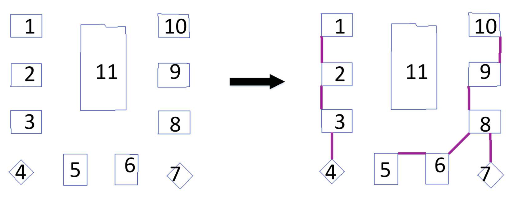
3.2. Group Obstacles
This section introduces the method for grouping obstacles by using the MD between them. Obstacles with bottlenecks (
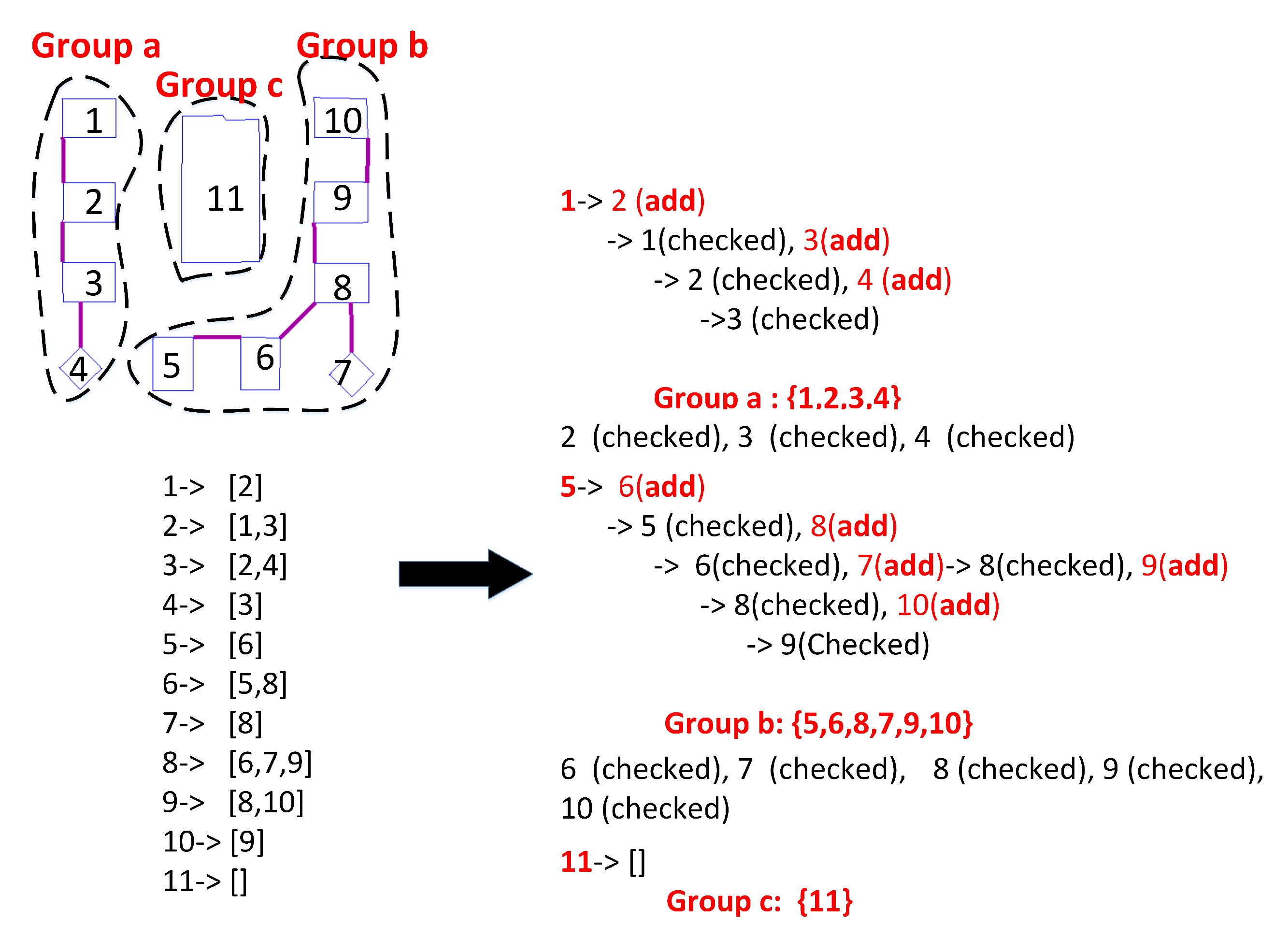
i.e., the MDs are smaller than a user’s dimensions) are put into a group. We create a linked list for each obstacle. Each bottleneck between two obstacles is regarded as a connection of them. The linked list contains all of the other connected obstacles. The following steps illustrate the process (see
Figure 7).
Step 1. Pick an unchecked obstacle as the current obstacle obs. If there is no unchecked obstacle, then go to Step 5. Otherwise, create an empty group gop; add obs to gop; and go to Step 2.
Step 2. In the linked list of obs, add all of the unchecked members to gop.
Step 3. For the previously-added members, add all of the unchecked members in their linked lists to the gop.
Step 4. Repeat Step 3 until no unchecked members are found. Then, the obstacles in the gop form a group. Go to Step 1.
Step 5. All of the groups have been identified. Count the number of groups and assign each group an ID.
Figure 7.
Grouping 11 obstacles into three groups with respect to the bottlenecks.
Figure 7.
Grouping 11 obstacles into three groups with respect to the bottlenecks.
Figure 7 presents an example of grouping obstacles. The groups of obstacles are the actual obstacles for the user with the given dimension. The user has to avoid the obstacle groups that can have different shapes. Accordingly, the boundary of every obstacle group needs to be generated, which will be addressed in
Section 3.4.
3.3. Select Obstacle Groups
This step is introduced to reduce the number of groups that will be used for path computation. Between two locations, some indoor objects may not interfere with the path for a user with a given dimension. Hence, we aimed to ascertain the groups of obstacles that influence a path.
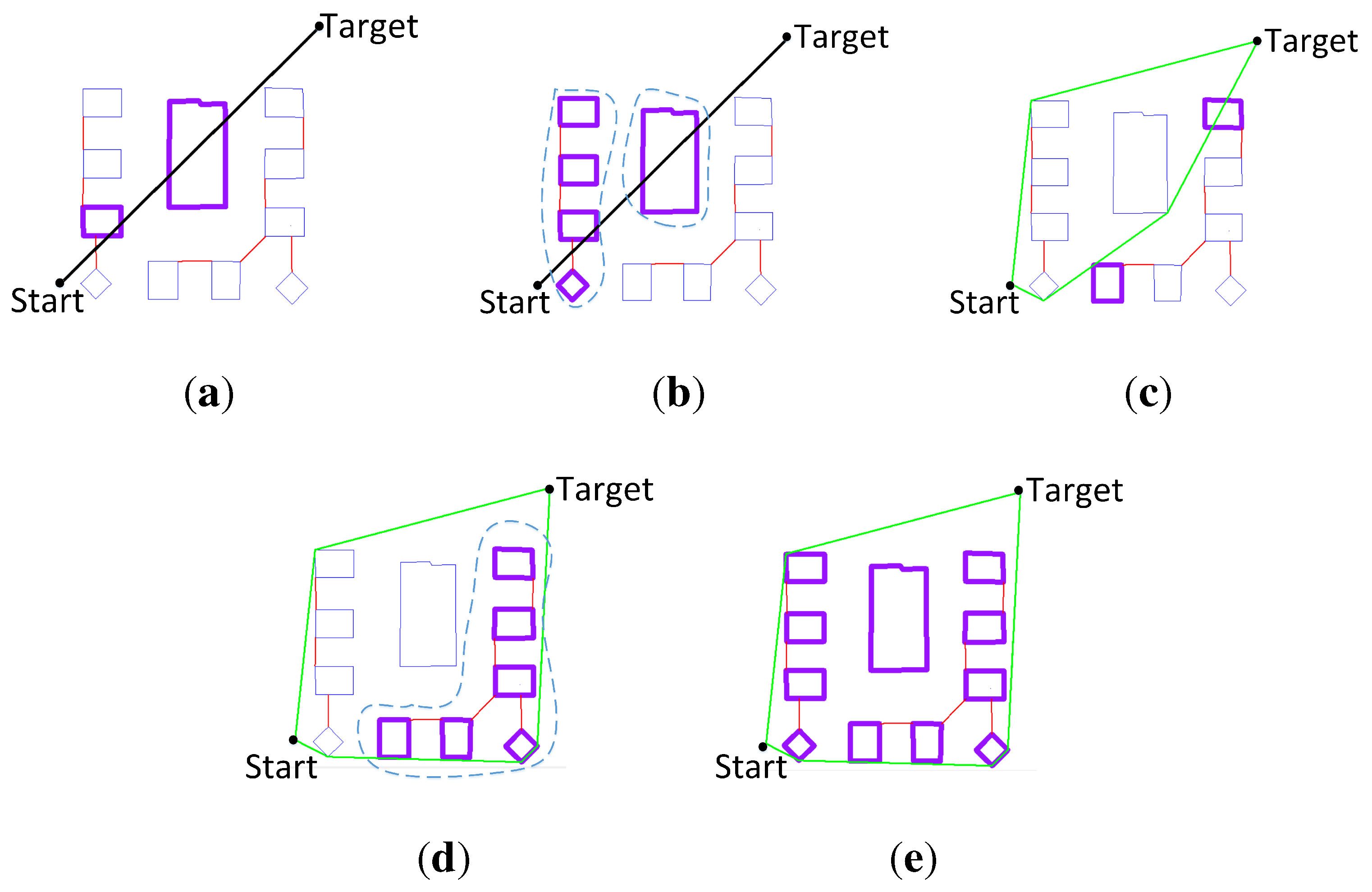
In a room, we compute first the shortest path between two locations without respect to the obstacles. The path is named the direct path. The direct path and CH of obstacles are employed to select obstacle groups. The selection process consists of the following steps.
Step 1. Find the obstacles intersecting the direct path.
Step 2. Select all of the obstacles from the groups that have an obstacle intersecting the direct path.
Step 3. Compute a CH with the nodes of all of the selected obstacles and the direct path.
Step 4. If the current CH intersects or contains new obstacles, look up the groups of the new obstacles, and select all of the obstacles from the new groups. Re-compute a CH.
Step 5. Iterate Step 4 until there are no other obstacles included by the current CH.
The obstacle selection aims to choose obstacle groups in a limited region for path finding. The iterative procedure will stop when the final CH (FCH) does not include any new obstacle. For a user with a given size, a path can be found in the FCH.
Figure 8.
Selecting obstacle groups with respect to the start and target location of a user. (a) The direct path intersects two obstacles; (b) selecting the groups of the intersected obstacles; (c) computing a convex hull (CH), and the CH intersects other obstacles; (d) selecting the group of new obstacles in and re-computing the CH; (e) no more obstacles intersect the CH, and then, three groups are selected.
Figure 8 illustrates the selection process. The obstacles have been grouped according to a given dimension of users. A direct path is computed between two locations. First, the direct path intersects two obstacles (Step 1). The two obstacles belong to two different groups; second, all of the obstacles in the two groups are selected (Step 2); third, a CH is computed with the selected obstacles (Step 3). Then, the CH intersects two new obstacles; fourth, the group of the two new obstacles is found. All of the obstacles in the group are selected, and then, a new CH is computed (Step 4); finally, the new CH has no other intersections (Step 5). Thus, the CH is the FCH, and the three groups of obstacles are selected.
The extreme case is that all of the obstacles in a room are selected in the FCH. This means that all of the obstacles will be used for path-finding. This case may happen in an obstacle-dense scenario. Large dimensions of humans and equipment can also result in the extreme case. Yet, in common indoor scenarios, only some of the obstacles in a room are selected.
3.4. Create Boundaries for Selected Groups
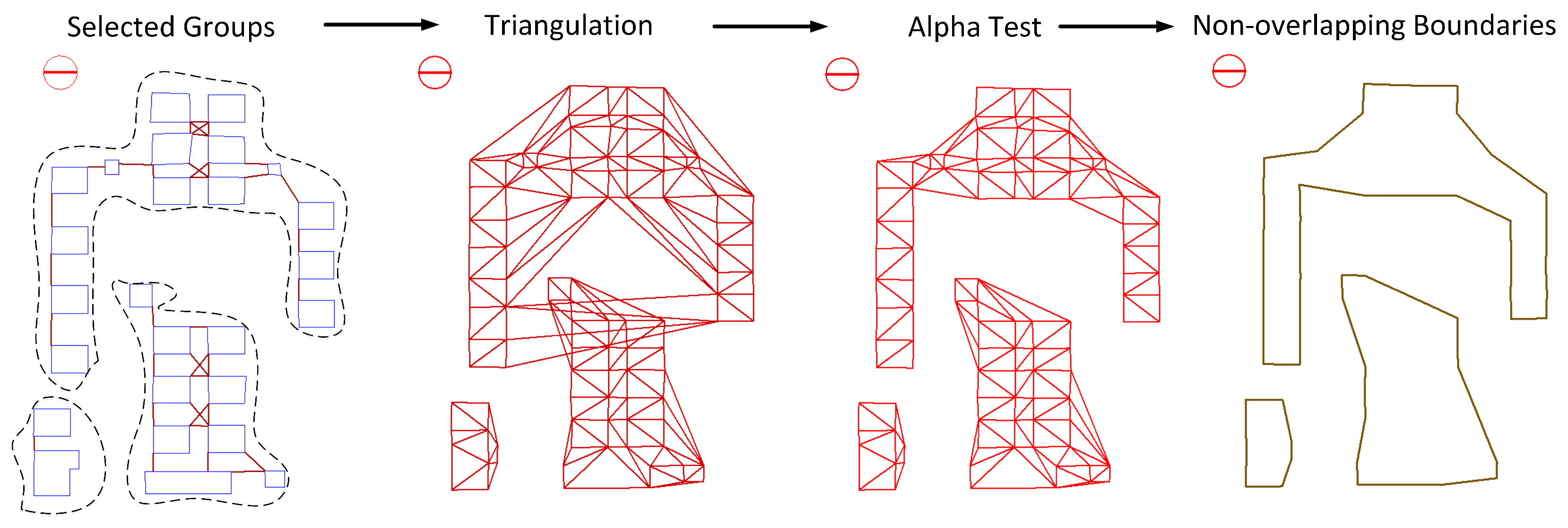
This section presents the generation of non-overlapping boundaries for the selected obstacle groups. The boundary of an obstacle group is an alpha shape of the vertices of all of the obstacles in the group. We computed the alpha shape based on the DT of the vertices (see
Section 2) and an alpha value. The alpha value is equal to the given dimension of a user. As a result, there is only one alpha shape (
i.e., the boundary) for the user. This method generates non-overlapping boundaries of all obstacle groups (see
Figure 9). The procedure for boundary generation is presented below.
Step 1. For a selected obstacle group, check the number of obstacles. If the group includes only one obstacle, then the obstacle’s polygon is the boundary. Otherwise, go to Step 2.
Step 2. Create a DT with the vertices of all obstacles in the group, and assign the given dimension of the user to the alpha value.
Step 3. Compute all of the lengths of edges of each triangle in the DT. Preserve a triangle if its edges’ lengths are all less than the alpha value.
Step 4. In all of the preserved triangles, find the edges only used for one triangle. Form the edges into a boundary.
Figure 9.
Resulting non-overlapping boundaries of obstacle groups.
Figure 9.
Resulting non-overlapping boundaries of obstacle groups.
Three groups of obstacles are shown in
Figure 10. The boundaries are derived in the same number of obstacle groups. The alpha value is set to 0.8 meters (m). At first, two groups’ DTs overlap. After the alpha test has been applied to the DTs, non-overlapping boundaries are computed for the groups.
Figure 10.
The boundary generation of three obstacle groups for a user with a size of 0.8 m.
Figure 10.
The boundary generation of three obstacle groups for a user with a size of 0.8 m.
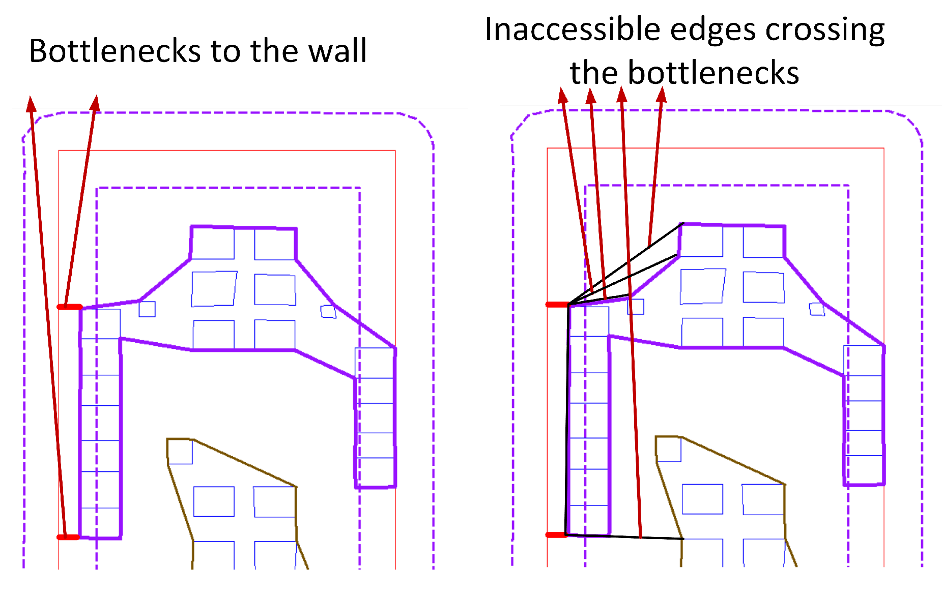
3.5. Create a Network Considering Inaccessible Gaps with Walls
There are two possibilities for paths for a user. Paths can be found either in the gaps between the groups of obstacles or the gaps between obstacles and walls of a room. If such a path is not found, this room cannot be passed by the user.
Similar to the bottlenecks between obstacles, we define the bottlenecks to a wall as the inaccessible gap between the wall and the boundary of an obstacle group. For a user with a given dimension, we detect the bottlenecks to walls by using the buffer of a room (see
Figure 11). The buffer is computed with the offset value equal to the user’s width. In the selected obstacle groups, if a node of the boundary is inside the buffer, then we compute a perpendicular line to the wall (see
Figure 11). The perpendicular line represents the bottleneck to the wall.
Figure 11.
Detecting bottlenecks between a wall and the boundary of an obstacle group and identifying inaccessible edges crossing the bottlenecks.
Figure 11.
Detecting bottlenecks between a wall and the boundary of an obstacle group and identifying inaccessible edges crossing the bottlenecks.
For a user with the given dimension, a network (e.g., VG) can be created in a room with the boundaries of the selected obstacle groups. The edges crossing the bottlenecks to the walls are inaccessible to the user (see
Figure 11). The edges would be removed for path computation.
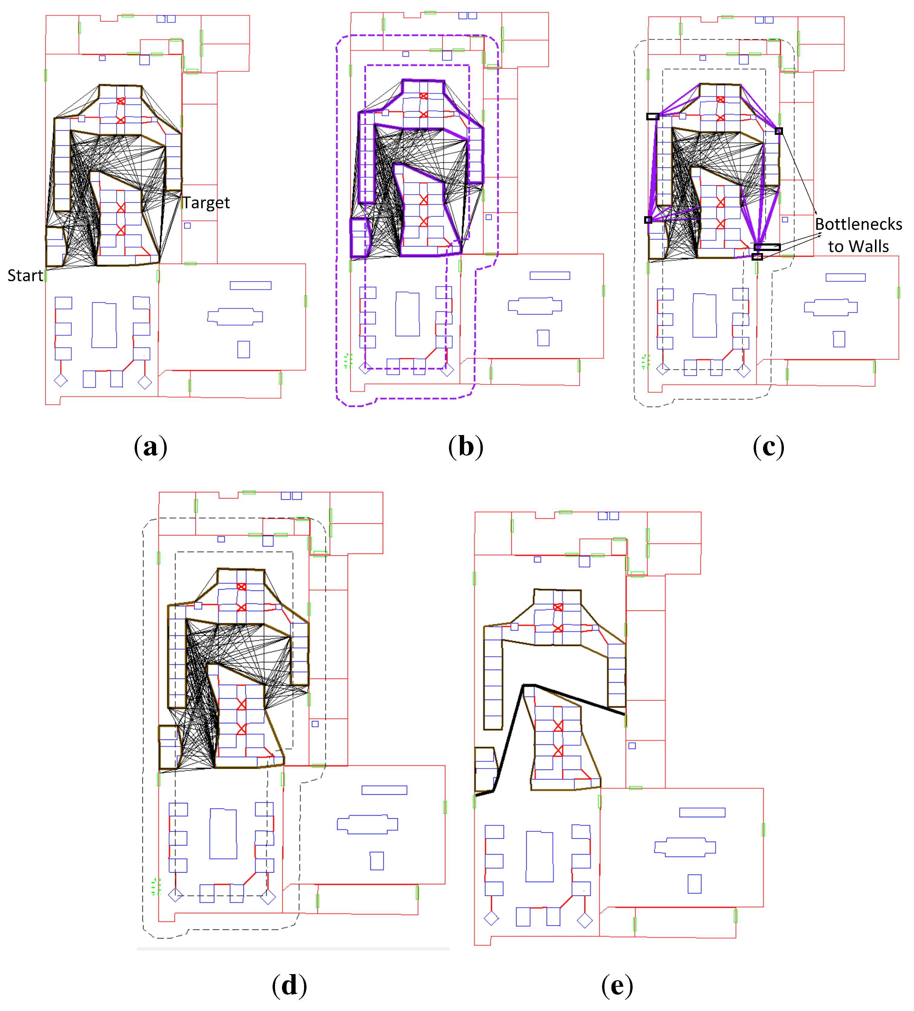
We adopted the VG as the navigation network.
Figure 12 illustrates the creation of the VG and presents the shortest path between two locations for users of 0.8 m. First, the VG is created with the nodes of three boundaries (see
Figure 12a). Second, a buffer of the room is computed, and the three boundaries overlap the buffer (see
Figure 12b). Third, all of the bottlenecks between the boundaries and walls are found (see
Figure 12c). Consequently, the inaccessible visibility edges are located. Fourth, the inaccessible visibility edges are removed (see
Figure 12d). Finally, the shortest path (see
Figure 12e) is computed in the VG. A user with the given size can follow the path.
Figure 12.
Creating a visibility graph (VG) and a room buffer, removing the inaccessible edges and computing a path for users with a size of 0.8 m. (a) Creating a VG; (b) computing a room buffer; (c) finding inaccessible edges in the bottlenecks; (d) removing the inaccessible edges; (e) the computed path.
4. Use Cases
The proposed method, including computing MDs, grouping obstacles, selecting obstacle groups, creating boundaries and creating VGs, was implemented by the C++ language within the Visual Studio 10.0 environment. We visualized the test results in the software MicroStation V8i of Bentley Systems.
This paper tested the proposed approach in two use cases on real floor plans: (1) a floor plan of a conventional neonatal intensive care unit (CNICU) at Sanford Children’s Hospital [
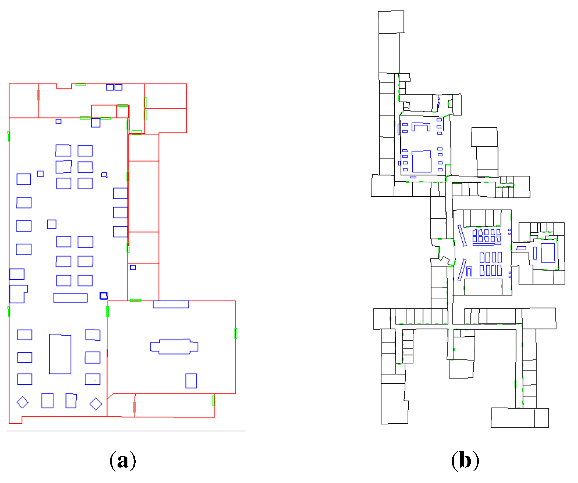
38]; and (2) the ground floor plan of the Architecture Faculty building at Delft University of Technology. They include a number of indoor objects (e.g., furniture), which are shown in
Figure 13. We computed different paths in the two floor plans.
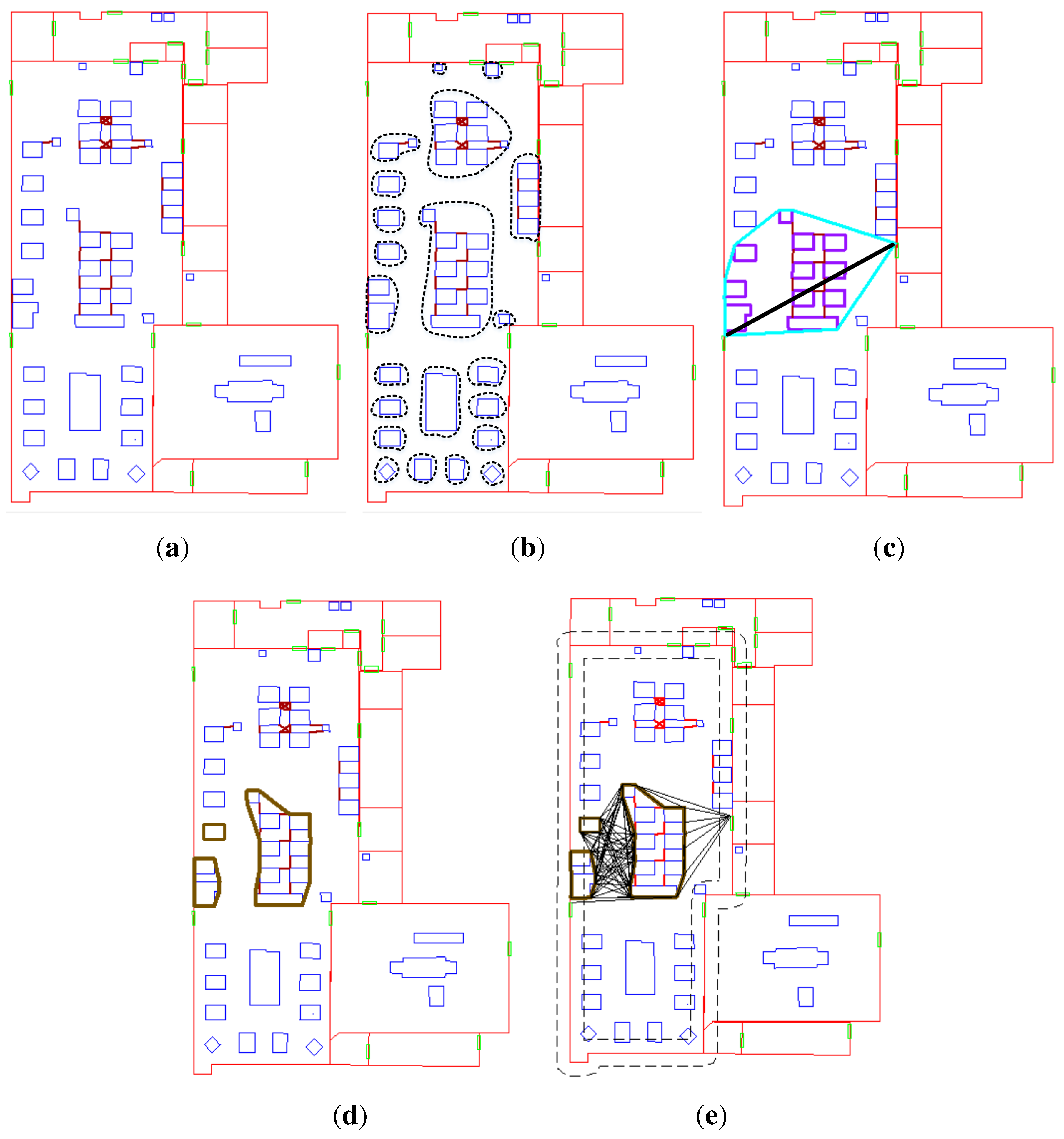
The first test is in the CNICU floor plan (
Figure 13a). We conducted the proposed method for a user with a size of 0.6 m (see
Figure 14). After we computed all of the MDs between the obstacles in the room and the bottlenecks, we ended the computation with 22 groups in total (see
Figure 14b). We selected three groups (see
Figure 14c) in the FCH between two doors and created the non-overlapping boundaries of the three groups (see
Figure 14d). The VGs based on the three boundaries and the buffer of the room were computed. As two boundaries overlap the buffer, we removed the inaccessible edges of the VG (see
Figure 14e). Consequently, we computed a path for the user in this VG.
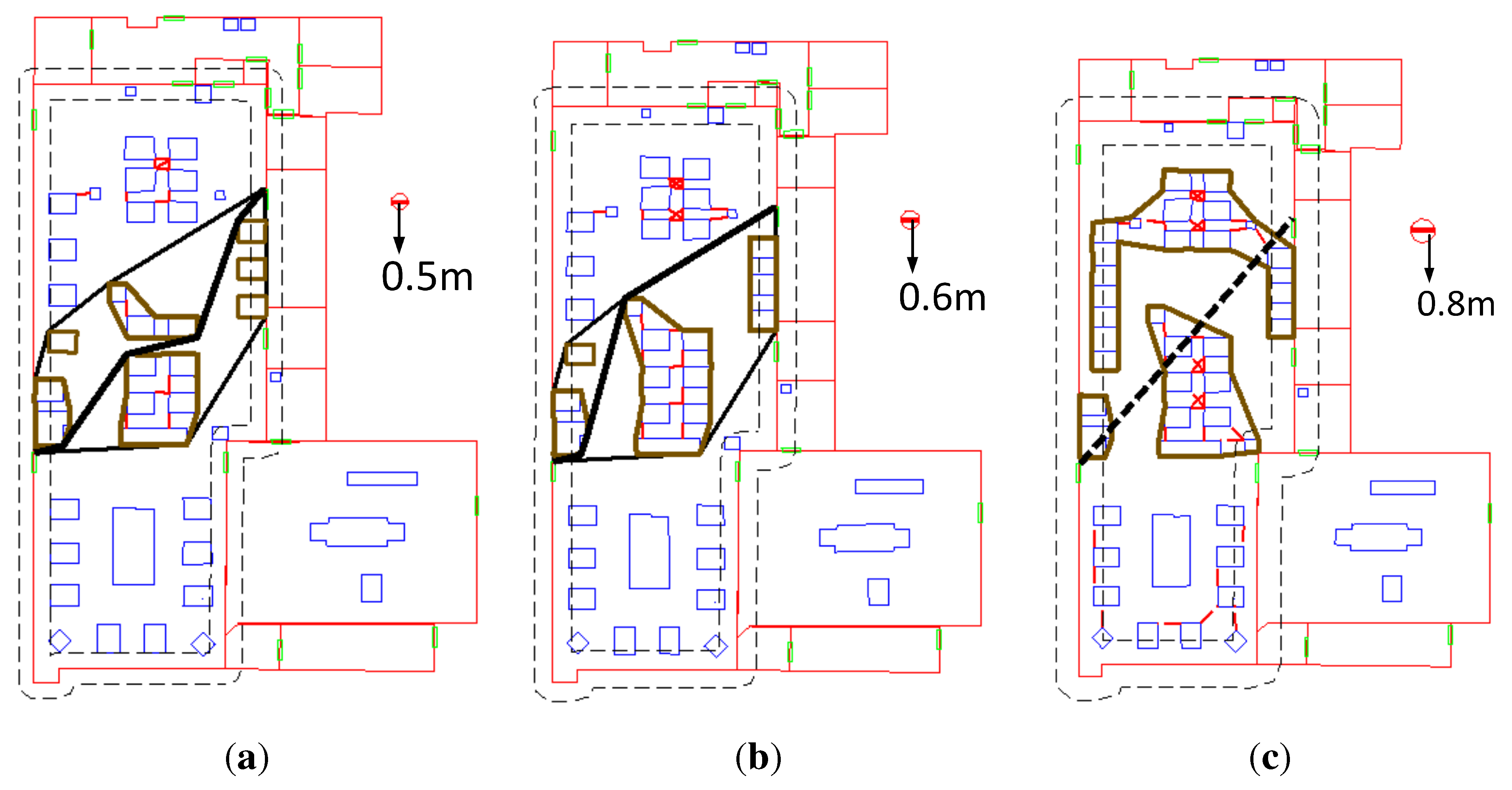
Here, we present different paths with respect to three sizes of user: 0.5 m, 0.6 m and 0.8 m. In
Figure 15a, the shortest path for 0.5 m lies in the middle of the FCH between two doors.
Figure 15b shows the path for 0.6 m. For the user of 0.6 m, a part of the path is on the FCH (see
Figure 15b). There is no path for the user of 0.8 m (see
Figure 15c). The computed buffer to the room’s walls overlaps with the boundaries of the three obstacle groups, and therefore, the user of 0.8 m cannot pass (see
Figure 15c).
Figure 13.
The floor plans of two buildings. (a) The floor of the conventional neonatal intensive care unit (CNICU) at the hospital; (b) ground floor of the Architecture Faculty building.
Figure 13.
The floor plans of two buildings. (a) The floor of the conventional neonatal intensive care unit (CNICU) at the hospital; (b) ground floor of the Architecture Faculty building.
In the other scenario (see
Figure 13b), we focused on one of the spaces including relatively dense obstacles (e.g., desks and pillars). Paths were computed with respect to three sizes of users: 0.5 m, 0.8 m and 1.0 m. Although the grouping results are different, the shortest paths for 0.5 m (see
Figure 16a) and for 0.8 m (see
Figure 16b) are the same. A user with a size of 1.0 m (see
Figure 16c) needs to follow another path.
Figure 14.
Testing the complete approach between two locations for a user with a size of 0.6 m. (a) Computing the bottlenecks between obstacles; (b) grouping the obstacles; (c) selecting obstacle groups; (d) creating the boundaries of the selected groups; (e) creating a VG and removing the inaccessible edges.
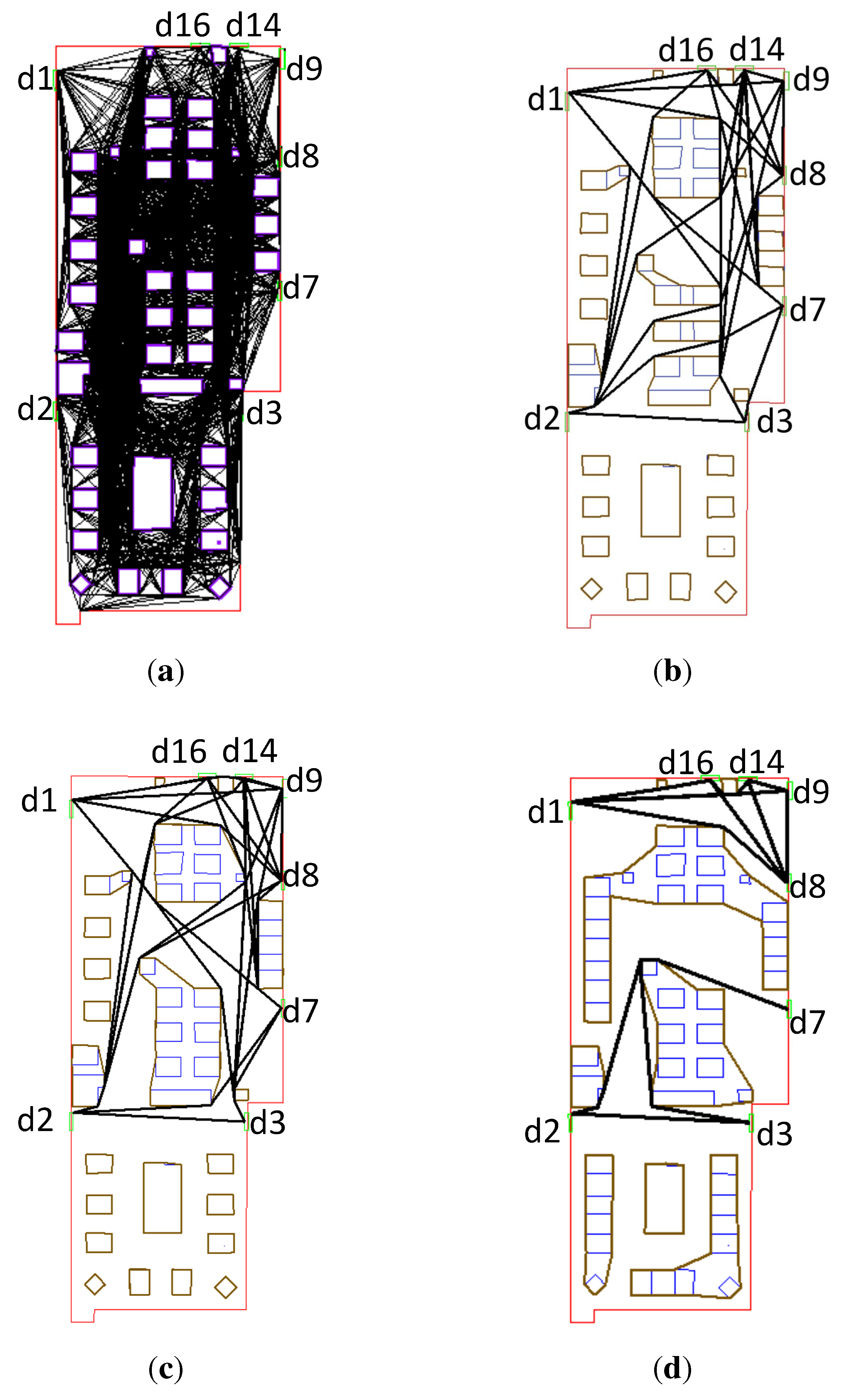
The proposed approach can be applied to precompute navigation networks for users with different dimensions.
Figure 17a presents the VG created with all obstacles without respect to a user’s dimension. The VG is complicated, and it cannot support path computation regarding a user’s dimension. In the proposed approach, we can omit the step “select obstacle groups” and create boundaries for all of the obstacle groups in a room. In this way, all of the shortest paths between the doors in the room can be computed (see
Figure 17). Three networks (
Figure 17b–d), consisting of the shortest paths between the doors, are precomputed for the users with the sizes of 0.5 m, 0.6 m, 0.8 m, respectively. For other users with the given dimensions, paths can be immediately provided for them in the networks. Moreover, the inaccessibility between doors can be recorded and be reported to the users. For instance, there is no path between the doors D2 and D8 for the users of 0.8 m (
Figure 17d), yet paths between the two doors exist for the users of 0.5 m and 0.6 m (
Figure 17b,c).
Figure 15.
Path-finding for the sizes of 0.5 m, 0.6 m and 0.8 m on the hospital floor plan. (a) The shortest path for the 0.5 m size; (b) the shortest path for the 0.6 m size; (c) no path for the 0.8 m size.
Figure 15.
Path-finding for the sizes of 0.5 m, 0.6 m and 0.8 m on the hospital floor plan. (a) The shortest path for the 0.5 m size; (b) the shortest path for the 0.6 m size; (c) no path for the 0.8 m size.
Figure 16.
The shortest paths for the sizes 0.5 m, 0.8 m and 1.0 m on the floor plan of the campus building. (a) Path for the 0.5 m size; (b) path for the 0.8 m size; (c) path for the 1.0 m size.
Figure 16.
The shortest paths for the sizes 0.5 m, 0.8 m and 1.0 m on the floor plan of the campus building. (a) Path for the 0.5 m size; (b) path for the 0.8 m size; (c) path for the 1.0 m size.
Figure 17.
(a) The VG regardless of a user’s dimension and (b–d) all of the shortest paths between all doors for the sizes of 0.5 m, 0.6 m and 0.8 m. (a) The complete VG of all obstacles without respect to a user’s dimension; (b) all of the shortest paths for the user with a size of 0.5 m; (c) all of the shortest paths for a user with a size of 0.6 m; (d) all of the shortest paths for the user with a size of 0.8 m.
5. Conclusions
In this paper, we proposed a new method to compute paths for users with different dimensions. The proposed method groups obstacles and replaces the groups with simple polygons. Compared to the Minkowski sum, this approach ensures that these polygons have no inner rings. The number of vertices to be considered for the construction of a navigation network is also significantly reduced. We have demonstrated that the proposed method can either compute a path to move through obstacles or report that no path can be found between the two locations. We have illustrated the proposed method in several use cases.
This approach can also be used to create navigation networks for users with different dimensions (see
Figure 17). For each user, all of the shortest paths between doors can be precomputed first. The networks of these paths can be maintained in a database and used according to path requests. The user can also be informed if no path exists. The accessibility information can even be recorded as the attribute to each room and employed for users to estimate generally the possibilities to pass through certain rooms.
This approach can be improved in several aspects. First, the MD between non-convex polygons should be considered, because the currently computed MDs might not be accurate in some cases. Presently, we compute the MD between the CHs of obstacles.
Figure 18 illustrates the the difference in the computed MD between a convex obstacle and the CH of a non-convex one. The genuine MD (
Figure 18b) between the two obstacles is larger than the computed one (
Figure 18a) derived from the current approach. In this case, when the computed MD indicates inaccessibility, the gap between the two obstacles might still be accessible for the user.
Figure 18.
The computed and genuine minimum distances (MDs) between a convex and a non-convex obstacle. (a) The computed MD in our approach; (b) the genuine MD.
Figure 18.
The computed and genuine minimum distances (MDs) between a convex and a non-convex obstacle. (a) The computed MD in our approach; (b) the genuine MD.
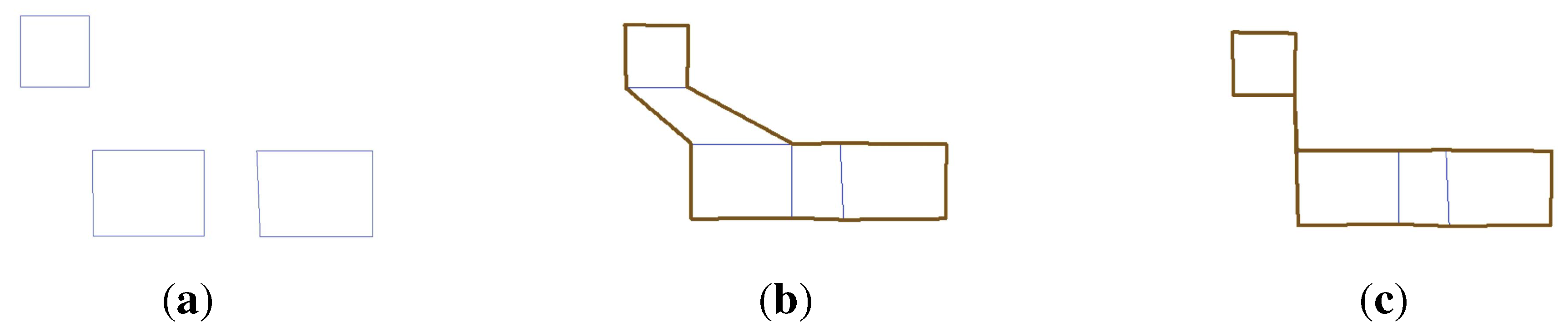
The second point is about creating the boundary of an obstacle group. Currently, the boundaries generated by our approach are not always the minimum outer boundary. For instance, the three obstacles (
Figure 19a) are in the same group.
Figure 19b illustrates the result of our approach. The obtained boundary is not the strict boundary of the three obstacles with the minimum area, but the boundary is a valid polygon (
i.e., no edges and vertices overlap). This boundary can be considered reasonable for humans, because people tend to avoid obstacles instead of heading into their inside. However, the strict boundary (
Figure 19c) might be more suitable for the motion-planning of robots, especially in the cases (e.g., robotic vacuum cleaners) where the entire free space around obstacles needs to be traversed.
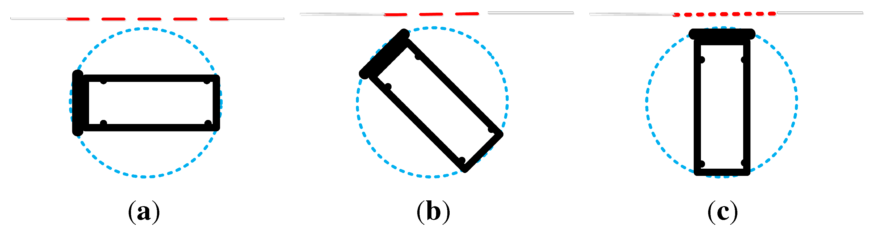
Currently, we simplify the user with equipment as a circle, which releases us from considering the rotation of users.
Figure 20a indicates that the gap in a wall can be passed by the user regardless of his or her orientation, because the diameter of the user is smaller than the gap.
Figure 20b shows that the user rotates a small angle, yet the gap cannot be traversed, since the diameter is larger than the current gap. When the user turns 90 degrees, the short side of the user is smaller than the gap. The user can still pass through the gap, though the diameter is larger than the gap. We could consider the minimum size of the user and obtain a path that would offer more options for passing, but then, we would have to ensure that enough space is available for rotating the equipment in front of the bottleneck. This would require the enhancement of our approach to indicate the timing when the user has to rotate for passing a bottleneck.
Figure 19.
The boundaries of three obstacles in our method and in a strict condition. (a) Three obstacles; (b) our boundary for the group of three obstacles; (c) a strict boundary for the group of three obstacles.
Figure 19.
The boundaries of three obstacles in our method and in a strict condition. (a) Three obstacles; (b) our boundary for the group of three obstacles; (c) a strict boundary for the group of three obstacles.
Figure 20.
(a) A user can pass through a gap larger than the diameter of the user’s circle; (b) the user cannot pass through the gap when the diameter is larger; and (c) the user can pass through the gap after a 90-degree turn. (a) The user can pass through the gap when its length is longer than the diameter of the circle; (b) the user cannot pass the gap when its length is shorter than the diameter of the circle; (c) the user can pass through the gap because the user’s short side is smaller than the gap, though the diameter of the circle is larger than the gap.
In the future, the MD between non-convex polygons will be taken into account. Then, the bottlenecks between obstacles will be better estimated. We also intend to investigate how the boundary-generation method can be improved. The computed boundaries of obstacle groups need to approximate the strict ones without losing their validity. Furthermore, we will investigate how the real shape of a user (with equipment) can be considered.
Another interesting topic for future work is the path computation considering moving objects. For instance, the moving objects can be tracked and their shapes can be updated on the floor plan in different time slots. We can apply our method frequently in different time slots to update the path maps (e.g., the ones in
Figure 17). The details will be investigated in the future.
At the moment, the proposed approach is considered for one room, and paths can be computed between any two locations in one room. No attention has been paid to the case of paths between two locations in distinct rooms. If there are multiple doors between two neighboring rooms, we have to select a door from the multiple options. Future research should investigate the selection of the door into the next room.


