The findings of this study include classification of accuracy assessment from WV2 imagery, classification image, DDP, and association between the roofs and the DDP.
3.1. Accuracy Assessment of Roof Classification
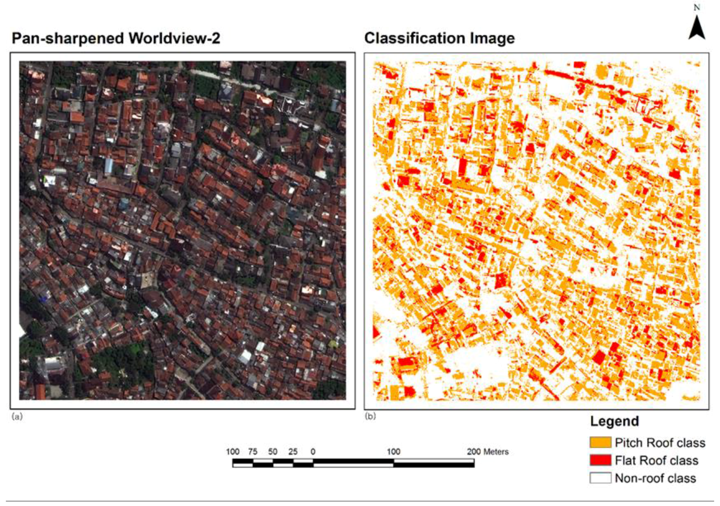
The classification accuracy was evaluated using a confusion matrix based on the classification result for the ROIs. Herewith, the Supervised Minimum Distance classifier was applied to the pan-sharpened WV2 imagery. Results in
Table 2 suggest moderate agreement (0.4–0.8) on Kappa coefficient (KC) [
45] with 70.59% overall accuracy (OA), less than the previous study, which also produced a confusion matrix for WV2 images and which found 87.87% user accuracy and 77.91% producer accuracy for the roof class [
46]. However, 81.47% OA with 0.75 KC of their study is categorized as moderate agreement, which is in line with results of the present study.
Figure 4 was produced to show the RGB color composite of the pan-sharpened image and the classification image.
This classification image resulted only from the R, G, B color composite, whereas in another study that performed WV2 band of R, G, and B, the near-infra-red (NIR) and panchromatic (PAN) band found 71.3% OA and 0.59 KC, which suggests a similar manner with this study (70.59% OA and 0.51 KC) [
20]. We did not use Google Earth image because it only provides visual representation of possible dengue breeding sites of an image and is lacking of automated extract feature as well as land cover analysis [
43].
Table 2.
Confusion matrix for classification accuracy assessment.
Table 2.
Confusion matrix for classification accuracy assessment.
| Classified Data | Reference Data | User Accuracy (%) |
|---|
| Pitched Roof | Flat Roof | Non-Roof | Total |
|---|
| Pitched Roof | 34 | 7 | 47 | 88 | 38.64 |
| Flat Roof | 3 | 41 | 5 | 49 | 83.67 |
| Non-Roof | 15 | 3 | 117 | 135 | 86.67 |
| Total | 52 | 51 | 169 | 272 | |
| Producer accuracy (%) | 65.38 | 80.39 | 69.23 | | |
| Overall accuracy % | 70.59 | | | | |
| Kappa coefficient | 0.51 | | | | |
Figure 4.
(a) RGB color composite of pan-sharpened 2 and (b) PR, FR, and NR class image.
Figure 4.
(a) RGB color composite of pan-sharpened 2 and (b) PR, FR, and NR class image.
3.3. OLS Regression and GWR Model
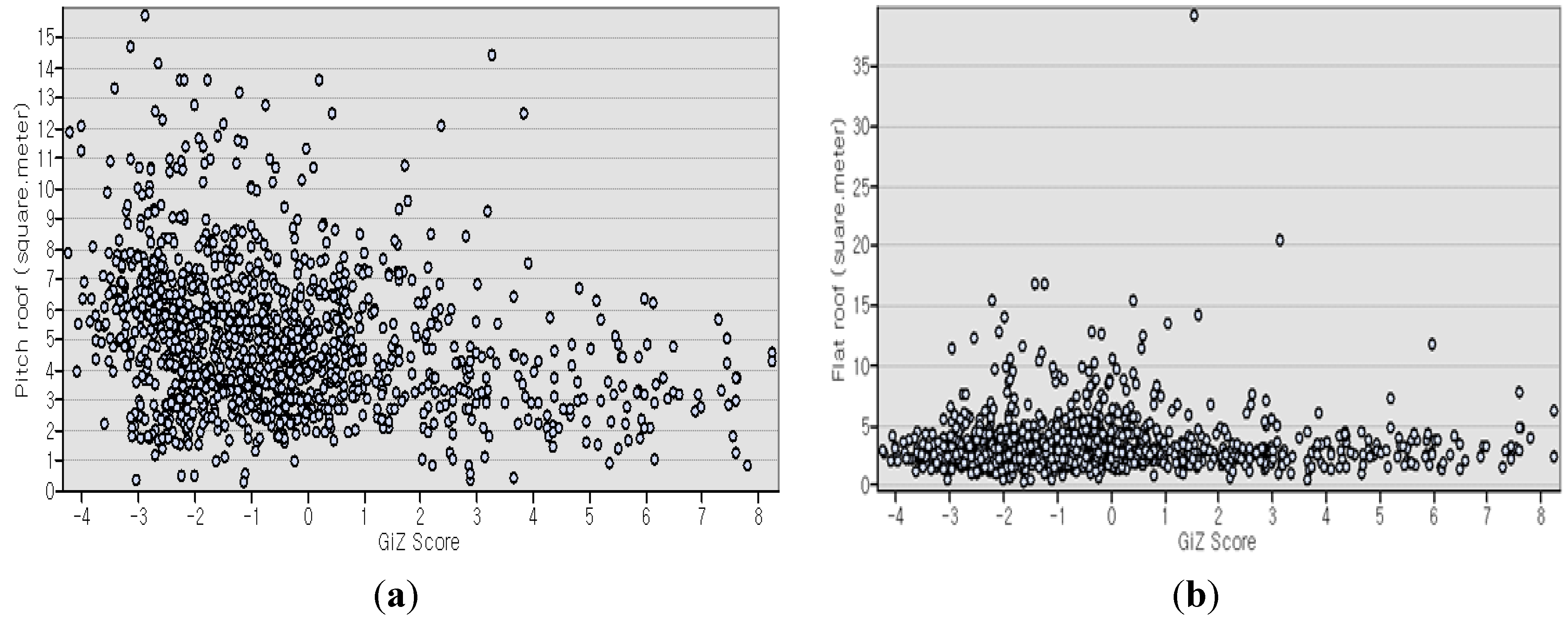
The scatter plot of PR and FR to GiZ scores is depicted in
Figure 6. Some FR plots are visible as outliers. We defined them as outliers after the scatter plot results shown, from which we observed which data were separated and suspected as outliers. We tested them by comparing
R2, adjusted
R2, and AICc for all data, and the whole data minus the outliers. The criteria were that if
R2, adjusted
R2, and AICc of all data are higher than if without the suspected outliers, then they are not outliers; and if it is lower, then we designated them as outliers. From OLS regression analysis, we found positive autocorrelation (Moran’s Index = 0.67,
p = 0.000).
Table 4a shows that the data are not mutually redundant (VIF < 10) and non-stationary at all points (Koenker test = 0.00). From all DDP data, we found that smaller PR size and larger FR size were associated with increasing DDP into a more clustered trend or into positive directions of GiZ score (OLS: PR value = −0.27; FR= 0.04;
R2 = 0.076; GWR:
R2 = 0.76). We then divided all data into three groups: hotspot, random, and dispersed patterns, as shown respectively in
Table 4. In the hotspot pattern, we excluded the outlier because it resulted in a higher measurement value on
R2 and adjusted
R2, and a lower value of AICc after the exclusion. However, we included the outliers of random patterns because, as presented in
Table 4b, OLS regression measurement test results on
R2 and adjusted
R2 were higher with outliers than without outliers, even though AICc showed a lower value without outliers. In each pattern, we analyzed the association, which revealed that PR had more negative values and that FR had more positive values in hotspots than others (OLS: PR value = −0.17, FR = 0.14,
R2 = 0.06 in hotspot pattern; PR value = −0.01, FR= 0.03,
R2 = 0.01 in random pattern; and PR value = −0.04, FR = 0.02,
R2 = 0.04 in dispersed pattern).
Figure 6.
(a) Scatter plot of PR with GiZ score and (b) scatter plot of FR with GiZ score.
Figure 6.
(a) Scatter plot of PR with GiZ score and (b) scatter plot of FR with GiZ score.
Of the OLS estimated values, PR was all in negative values. It corresponds with the observation that the smaller the size of the PR was, the higher the GiZ score or the higher the trend was in the higher clustered pattern. In contrast, FR was found in positive estimated values, implying that larger FR showed a stronger trend of becoming a higher clustered pattern. Assuming most of the PR were also with FR based on visual interpretation, this condition might result from lower water flow velocity on FR [
17].
Moreover, stagnant water caused by blocked roof gutters makes a productive habitat for
Aedes mosquito breeding [
8,
18]. Regarding the smaller size of PR, it might be associated with densely populated areas where most dengue disease incidence was found. Although many studies have done detailed mapping of homes, results are very rarely related to dengue incidence [
43].
Another potential explanation results from more difficult access to cleaning the gutters of smaller PR. Unfortunately, we were unable to find a report to refute or corroborate this explanation. An earlier study found that it was uncommon behavior to clean a roof gutter, but no mention of the difficulty of accessing smaller PR is forthcoming from the literature [
8]. From a behavior perspective, untidy and poorly maintained houses, yard, and larger shade conditions present a high risk of dengue disease because female
Aedes mosquitoes are more attracted to such houses where more breeding sites are often available [
47,
48].
Table 4.
(a) Ordinary least squares (OLS) regression and geographically weighted regression (GWR) model: all and hotspot. (b) OLS regression and GWR model: random. (c) OLS regression and GWR model: dispersed.
(a)
| Parameter | All | Hotspot |
|---|
| Estimated Value | Std. Error | p Value | VIF | Estimated Value | Std. Error | p Value | VIF |
|---|
| OLS | GWR | | | | OLS | GWR | OLS | OLS | OLS |
|---|
| | | | | Outlier | Outlier | Outlier | Outlier | Outlier |
|---|
| | | | | with | without | without | with | without | with | without | with | without |
|---|
| Number of observations | 1154 | 1154 | 1154 | 1154 | 1154 | 184 | 183 | 183 | 184 | 183 | 184 | 183 | 184 | 183 |
| Intercept | 0.81 | | 0.18 | 0.00 | | 4.46 | 4.23 | | 0.33 | 0.36 | 0.00 | 0.00 | | |
| Pitched roof | −0.27 | | 0.03 | 0.00 | 1.00 | −0.16 | −0.17 | | 0.06 | 0.06 | 0.00 | 0.00 | 1.00 | 1.00 |
| Flat roof | 0.04 | | 0.03 | 0.00 | 1.00 | 0.05 | 0.14 | | 0.06 | 0.08 | 0.52 | 0.12 | 1.00 | 1.00 |
| R2 | 0.076 | 0.76 | | | | 0.04 | 0.06 | 0.39 | | | | | | |
| Adjusted R2 | 0.075 | 0.75 | | | | 0.03 | 0.05 | 0.30 | | | | | | |
| AICc | 5184.97 | 3709.59 | | | | 723 | 717.7 | 670.30 | | | | | | |
| Koenker test | 29.99 | | | 0.00 | | 3.68 | 3.58 | | | | 0.16 | 0.17 | | |
| Jarque-Bera | 320.22 | | | 0.00 | | 15.1 | 14.02 | | | | 0.00 | 0.00 | | |
(b)
| Parameter | Random |
|---|
| Estimated Value | Std. Error | p Value | VIF |
|---|
| OLS | GWR | OLS | OLS | OLS |
|---|
| Outlier | Outlier | Outlier | Outlier | Outlier |
|---|
| with | without | with | with | without | with | without | with | without |
|---|
| Number of observations | 555 | 554 | 555 | 555 | 554 | 555 | 554 | 555 | 554 |
| Intercept | −0.30 | −0.27 | | 0.10 | 0.10 | 0.00 | 0.00 | | |
| Pitched roof | −0.01 | −0.01 | | 0.02 | 0.02 | 0.36 | 0.36 | 1.00 | 1.00 |
| Flat roof | 0.03 | 0.02 | | 0.01 | 0.02 | 0.05 | 0.30 | 1.00 | 1.00 |
| R2 | 0.01 | 0.004 | 0.37 | | | | | |
| Adjusted R2 | 0.01 | 0.000 | 0.32 | | | | | |
| AICc | 1376.14 | 1373.15 | 1179.64 | | | | | | |
| Koenker test | 0.53 | 0.90 | | | | 0.77 | 0.64 | | |
| Jarque-Bera | 23.04 | 23.52 | | | | 0.00 | 0.00 | | |
(c)
| Parameter | Dispersed |
|---|
| Estimated Value | Std. Error | p Value | VIF |
|---|
| OLS | GWR | OLS | OLS | OLS |
|---|
| Outlier | Outlier | Outlier | Outlier | Outlier |
|---|
| with | with | with | with | with |
|---|
| Number of observations | 415 | 415 | 415 | 415 | 415 |
| Intercept | −2.36 | | 0.08 | 0.00 | |
| Pitched roof | −0.04 | | 0.01 | 0.00 | 1.00 |
| Flat roof | 0.02 | | 0.01 | 0.04 | 1.00 |
| R2 | 0.04 | 0.23 | | | |
| Adjusted R2 | 0.04 | 0.18 | | | |
| AICc | 701.82 | 644.74 | | | |
| Koenker test | 10.40 | | | 0.006 | |
| Jarque-Bera | 18.22 | | | 0.00 | |
The OLS assumes that relationship is in random (stationary) distribution whereas in this study was not in random manner because the relation was also influenced by location which might have a different relation at each location [
36,
44]. When this phenomenon is found, OLS regression results suggest the use of a GWR model to measure the association because the OLS indicated a not-normal residual distribution (
p value of Jarque-Bera < 0.01). The summary results of GWR are presented in
Table 4. From all DDP data, we found that the relationship was higher when using GWR model (
R2 = 0.76). However, we considered focusing more on each local variations on dengue patterns as past studies found to distinguish relationships by local variations [
36,
44]. The association resulted in higher hotspot patterns than in random and dispersed patterns (GWR:
R2 in hotspot = 0.39, random = 0.37, dispersed = 0.23), which according to Kinear PR and Gray CD is a larger effect (<0.01, small effect; 0.01 to 0.1, medium, and >0.1 is a large effect) than that of the OLS results found as medium effect [
49]. Vanwambeke
et al. in their previous research about the presence of
Aedes sp. larva, found higher association (
R2 = 0.52) for peri-urban housing and orchards factors [
29]. Our limitation is that we were addressing only house roof variables, which indicated weaker results than those found by Vanwambeke
et al. Higher results might be obtained when adding vegetation and shadow as variables related to dengue disease [
29,
43,
47,
48]. We did not include them as dengue risk factors because we have added such variables with PR and FR variables in earlier experiments. Unfortunately, our HSR imagery showed low agreement between the classification image and ground data. Results might be attributable to the condition that we did not have a full bundle of imagery that consists of eight bands including the panchromatic band by which we can increase agreement using methods of past studies [
46]. We also did not have texture feature data of the city in a detailed manner, such as building and skyscraper textures. These data are crucially important when differentiating objects including shadows in HSR images [
20]. We also did not include precipitation data or temperature data as dengue disease risk, variables in the analyses because the climate station in the city that measured such data is lacking, although many researchers used such data in past studies [
11]. However, despite these limitations, this study specifically demonstrated the use of available HSR images from the Indonesian government, analyzed in automatic manner, with an attempt to integrate the data by relation with DDP. Different from previous studies, we analyzed DDP spatiotemporally based on mosquito characteristics: flight range and life cycle [
10,
11]. In future studies, manual digitation for the HSR imagery to correct the classification can be conducted to increase the agreement.
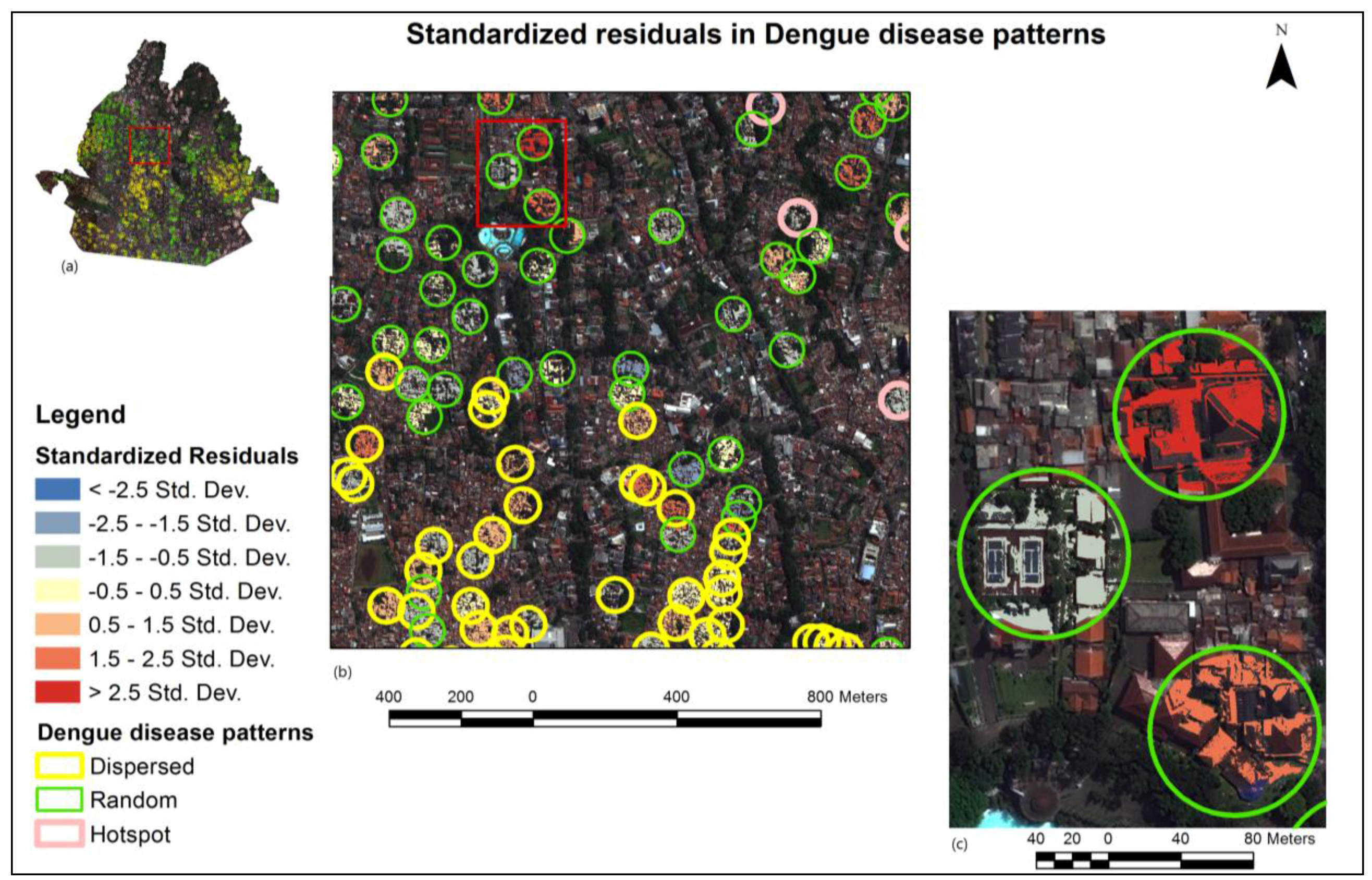
The standardized residual value of the GWR result is mapped in
Figure 7. This figure is presented to help set priorities to control roofs by cleaning them to prevent future dengue disease cases. Priority of the roof is any value closer to 0 (zero). The greater the difference of the value from 0 is, the lower its priority. If the value was more than 3 or less than −3, it was regarded as an outlier and was ignored [
49]. This point is crucially important for setting government priorities. Efforts can be more efficient and effective despite budget limitations.
Figure 7.
(a) Standardized residuals in DDP; (b) standardized residuals are shown within hotspot, random, and dispersed patterns; and (c) closer examination of the residuals on roofs.
Figure 7.
(a) Standardized residuals in DDP; (b) standardized residuals are shown within hotspot, random, and dispersed patterns; and (c) closer examination of the residuals on roofs.


 ,
, 


