1. Introduction
In the geomorphology sciences, mapping surface discontinuities that have appeared due to landslides is crucial to analyze the development of the displacement appropriately. The mentioned surface discontinuities are also referred to as surface fissures, which describe cracks and open fractures on the terrain. Different formations emerge from movements on the landslide surface, such as openings and slides, which can cause abrupt height changes across and along the fault lines. Different measurement methods can be applied to examine landslide fissures. For example, labor intensive field surveys provide sub-centimeter accuracy, which is the most precise method to extract features in detail. The field survey, however, is inadequate for the vast expanse of the ground in consideration of the long data collection time. Photogrammetric evaluation of the airborne images is an alternative surveying option, which is capable of obtaining topographic features of the vast landslide areas around sub-decimeter accuracy, depending on the camera capability and moderate flight heights. Products of aerial photogrammetry, such as the digital elevation model (DEM) and orthophotos are indispensable data sources in order to determine the kinematics of movements in the landslide regions with temporal monitoring, instead of extensive field survey [
1,
2].
In the last five years, the development of Unmanned Aerial Systems (UAS) have seen an improvement in the surveying techniques mentioned above as they produce highly accurate results but need a relatively short time for data capture. UAS-based photogrammetry, or remote sensing, is able to provide high accuracy data quickly using different sensor types, such as digital cameras, thermal cameras, multispectral cameras, and laser scanners. Current applications of UAS in geomatics can be categorized briefly as follows: agricultural and environmental applications, surveillance, aerial monitoring in engineering, cultural heritage, surveying, and cadastral applications [
3]. Particularly, in ground monitoring as a subfield of aerial monitoring in engineering, UAS-based photogrammetry has begun to play an important role in landslide monitoring and detection [
4,
5].
The increasing usage of UAS-based photogrammetric techniques has some considerable advantages in ground monitoring, when compared to the other terrestrial and airborne techniques. Lightweight, low-cost, high-resolution compact digital cameras of about 18–24 megapixels can be mounted easily to the drones producing high-quality aerial images from convenient flight heights. Then, the acquired images are evaluated to obtain high-density 3D data with low-cost photogrammetric software, e.g., Photomodeler Scanner [
6], Pix4D Mapper [
7], Agisoft PhotoScan [
8], or with open-source photogrammetric software, e.g., surface reconstruction from imagery (SURE) [
9], or patch-based multi-view stereo (PMVS) [
10] photogrammetric software [
11].
Another advantage of high-resolution imagery is the information, which is obtained from automatic feature extraction using low-level and high-level detection algorithms, such as corner detection, edge detection and motion detection. Detection algorithms are applied to images of different kinds of sensors in many disciplines. Digital images of the visible spectrum, thermal images, magnetic resonance imaging (MRI) images and high-resolution multispectral images can be used as the data source of automatic detection in medical, agricultural, and archeological research [
12,
13,
14]. Image processing methods for the fissure extraction also have a vital role in order to improve automatic detection of landslide fissures. The detailed contribution of the related works with regard to fissure extraction will be elaborated in this section.
Surface fissures are vital indicators for understanding and predicting slope movements [
15,
16]. Many researchers have tried to characterize and detect landslide fissures in order to provide information about the assessment of landslides [
17,
18]. In the last five years, UAS-based photogrammetric techniques have gained importance to model landslides appropriately. Niethammer
et al. [
19] identified fissures and displacements on the landslide surface using aerial images. Using the advantages of orthophotos, fissure structures and movement vectors can be defined. Image processing techniques that provide automatic data extraction and evaluation, however, were not used sufficiently in the research. Westoby
et al. [
20] proposed a low-cost photogrammetric method to produce a textured digital surface model to analyze different landforms for geosciences applications. Hugenholtz
et al. [
21] also explained the use of a UAS-based photogrammetric process for a digital terrain model and some basic landform feature extractions, using the maximum likelihood supervised classification. Cell-based or raster-based geomorphic feature extraction was applied, not only in landforms, but also in landslides to discover significant surface shapes [
22,
23].
Scientific research regarding landslide analysis can be discussed using two different scales. Works on a small scale cover wide land areas and mostly focus on producing susceptibility maps, while research on a large scale uses high-resolution data, such as UAS images and LIDAR data, to extract landslide triggered fissures. Studies for wide areas, as opposed to high-accuracy labor-intensive surveying methods, have improved quantification of landslide risks using regression and fuzzy approaches with many predictors, such as elevation, slope, aspect, lithology, land cover, distance to fault, distance to stream and distance to road [
24,
25,
26,
27].
However, these studies were limited to a general model that did not consider local explanations in detail for the regions. With the increasing availability of high-resolution data, with the latest generation of UAS providing aerial images having approximately 0.01 m GSD, automatic mapping of narrow fissure features has become feasible. Stumpf
et al. in the studies 2011 and 2013 [
28,
29] explained the use of the largely automated technique for the mapping of landslide surface fissures from very high-resolution aerial images. In the research, filtering algorithms and post-processing of the filtered images were implemented with airborne LIDAR data. In the 2012 study of Stumpf
et al. [
30], a multi-scale line detection approach was developed using UAS photographs as the only input, where a Gaussian matched filter (GMF) in combination with the first derivate of a Gaussian (FDOG) were considered.
Besides the research mentioned above, which focused on photogrammetry, LIDAR is also considered as the key technology to map landslides. Van den Eeckhaut
et al. [
31] proposed an object-based classification for the landslides from LIDAR derivatives to understand geomorphic processes from topographic signatures. Baruch and Filin [
32] presented an autonomous optimization driven model for fissure extraction and characterization using a multi-scale approach. Another approach introduced by Höfle
et al. [
33] described a method for the automatic delineation and geomorphometric description of fissures in cushion peat lands. The approach was a multi-step workflow, based on a fissure edge extraction and a sink filling algorithm applied to a conditioned digital terrain model. Although LIDAR is a suitable field method to derive DTMs in fissure research, airborne acquisition has drawbacks due to the high flight heights or costs. Furthermore, UAS imagery is often used as a high quality reference dataset to evaluate fissures for quantifying landslides.
Despite their lower resolutions compared to UAS imagery, satellite and aerial images as data sources have also been studied for fissure extraction by various researchers [
23,
34,
35,
36,
37,
38]. Youssef
et al. [
34] demonstrated the use of high-resolution satellite images using QuickBird imagery, acquired on 2 June 2007 (0.61 m spatial resolution), for detailed mapping of recent developments and slope instability hazard zones. Shruthi
et al. [
35] developed The Random Forests model from an object-oriented analysis using medium resolution ASTER images as the source of imagery information, combined with topographic information extracted from a DEM. In 2015, Shruthi
et al. [
36] made use of a semi-automatic object-oriented analysis to quantify changes in gully erosion areas over a period of eight years (2001 to 2009). Shruthi
et al. [
37] also investigated the use of object-oriented image analysis to extract erosion features, using a combination of topographic, spectral, shape (geometric) and contextual information obtained from satellite imagery. Conoscenti
et al. [
38] presented a characterization of susceptibility conditions using DEM and aerial images for gully erosion by means of GIS and multivariate statistical analysis.
Table 1 summarizes scales, precisions, and data sources of some mentioned scientific analyses.
Table 1.
The scope of some related works.
Table 1.
The scope of some related works.
| Article | Size | Precision | Data Source | Method |
|---|
| Stumpf et al. (2013) [29] | 14,000 m2 | 0.1 m | UAS images, airborne LIDAR | GMF, object oriented analysis |
| Stumpf et al. (2012) [30] | 1000 m2 | 0.1 m | UAS images | GMF |
| Baruch and Filin (2011) [32] | 1 km2 | 0.3 m | Airborne LIDAR | Multi-scale approach |
| Höfle et al. (2013) [33] | 1.8 km2 | 0.5 m | TLS | Edge extraction with sink filling |
| Shruthi et al. (2014) [35] | 80 km2 | 15 m | ASTER, GeoEye-1 | Object oriented analysis |
| Shruthi et al. (2015) [36] | 6 km2 | 1 m | Ikonos-2, GeoEye-1 | Object oriented analysis |
| Shruthi et al. (2011) [37] | 4 km2 | 1 m | Ikonos-2, GeoEye-1 | Object oriented analysis |
| Conoscenti et al. (2014) [38] | 9.5 km2 | 5 m | DEM / Aerial Photos | Logistic regression |
When related works are considered, to reason any information about a landslide from image-based analysis, it is clearly seen that feature extractions are applied to the images with particular accuracy. The lack of an appropriate data modeling approach decreases both accuracy and reasoning capability about the landslide field.
Considering the large amount of high-resolution data provided by UAS, this study focused on the development of an automatic image analysis technique to support landslide researchers in the detection, mapping and characterization of landslide surface fissures from UAS imagery. This paper presents and compares two methods involving integrating and modeling cell-based datasets for mapping surface fissures during the investigation of landslide dynamics. In the paper, an Adaptive Neuro Fuzzy Inference System (ANFIS), which integrates both neural networks and fuzzy logic principles, and a logical regression (LR) that uses statistical methods, were developed in order to estimate and validate the relationship between the high-resolution topographical features, based on dense 3D point clouds of the landslide surface, and the image data. The proposed models, taking advantage of the UAS imagery, eliminate many predictors, in contrast to the previous susceptibility landslides work that has been implemented across a wide range of fields. The determination coefficient (R2), root mean square error (RMSE), standard error of estimates (SEE) and receiver operation curve (ROC) were used as evaluation criteria to evaluate and compare the experimental results of ANFIS and LR using training and test datasets. The paper covers the workflow from beginning to end with regard to fissure extraction, which occurred as a result of landslide displacements. Subsequent to the model validation, the sufficiency of high-resolution UAS-based produced datasets, such as 3D point clouds, its cell-based derivatives, and orthophotos, are discussed to characterize landslide fissures.
2. Study Area
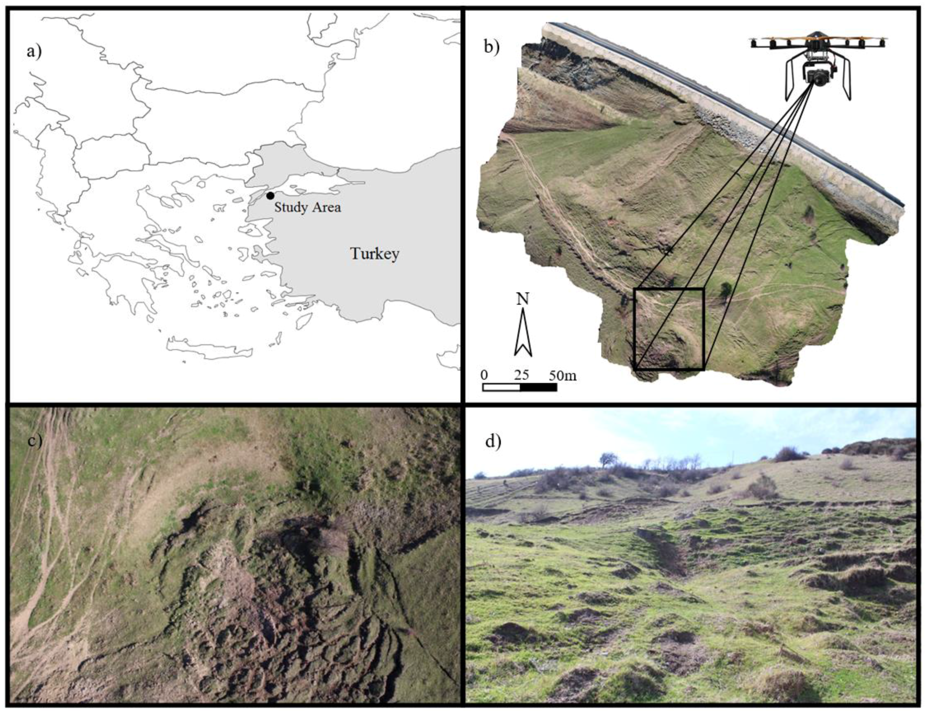
The processing approach was developed and tested in the area located next to Sevketiye village, Canakkale province on the coast southwest of Marmara, Turkey (
Figure 1). The total active area of the landslide covers approximately 10 hectares. The lower left WGS84 UTM coordinates of the area are 488,390 m East 4,471,630 m North and the upper left WGS84 UTM coordinates of the area are 488,590 m East 4,471,830 m North. The Canakkale–Bursa intercity high way, borders the area in the north and the average distance from the study area to the sea is around 150 meters.
Figure 1.
(a) Location of the study site; (b) the orthophoto of the landslide area and UAS with EOS M camera; (c) an aerial image of the landslide surface from the UAS; and (d) a terrestrial image of the landslide surface.
Figure 1.
(a) Location of the study site; (b) the orthophoto of the landslide area and UAS with EOS M camera; (c) an aerial image of the landslide surface from the UAS; and (d) a terrestrial image of the landslide surface.
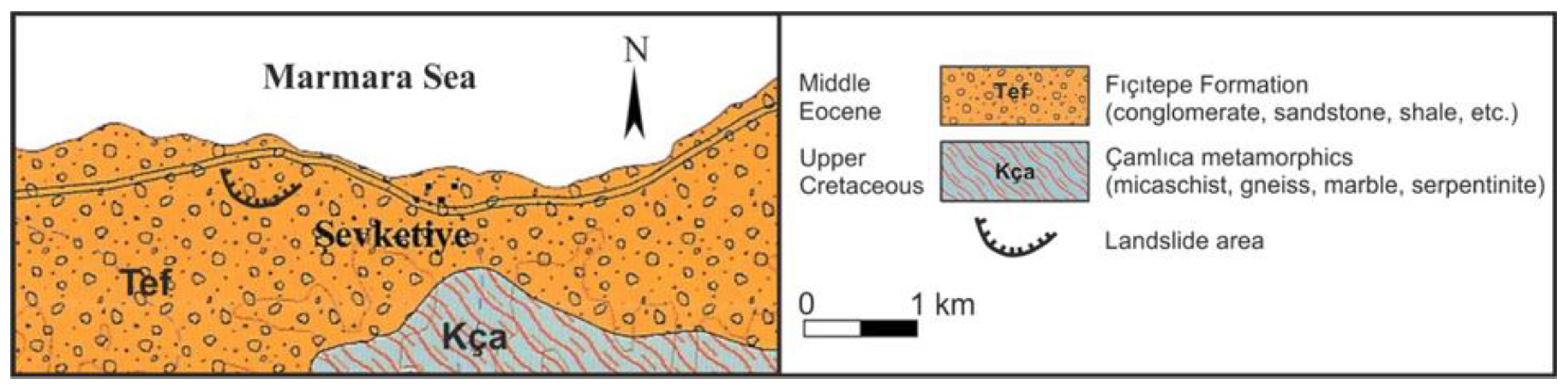
The geological units in the Sevketiye landslide and the surrounding areas consist of Cretaceous age metamorphic and Eocene sedimentary rocks, as illustrated in
Figure 2 [
39]. Basement rocks are unconformably overlain with sedimentary units. In the region, mass movements have occurred with regard to units of yellowish-brown sandstone and conglomerate that belong to the Fıçıtepe Formation [
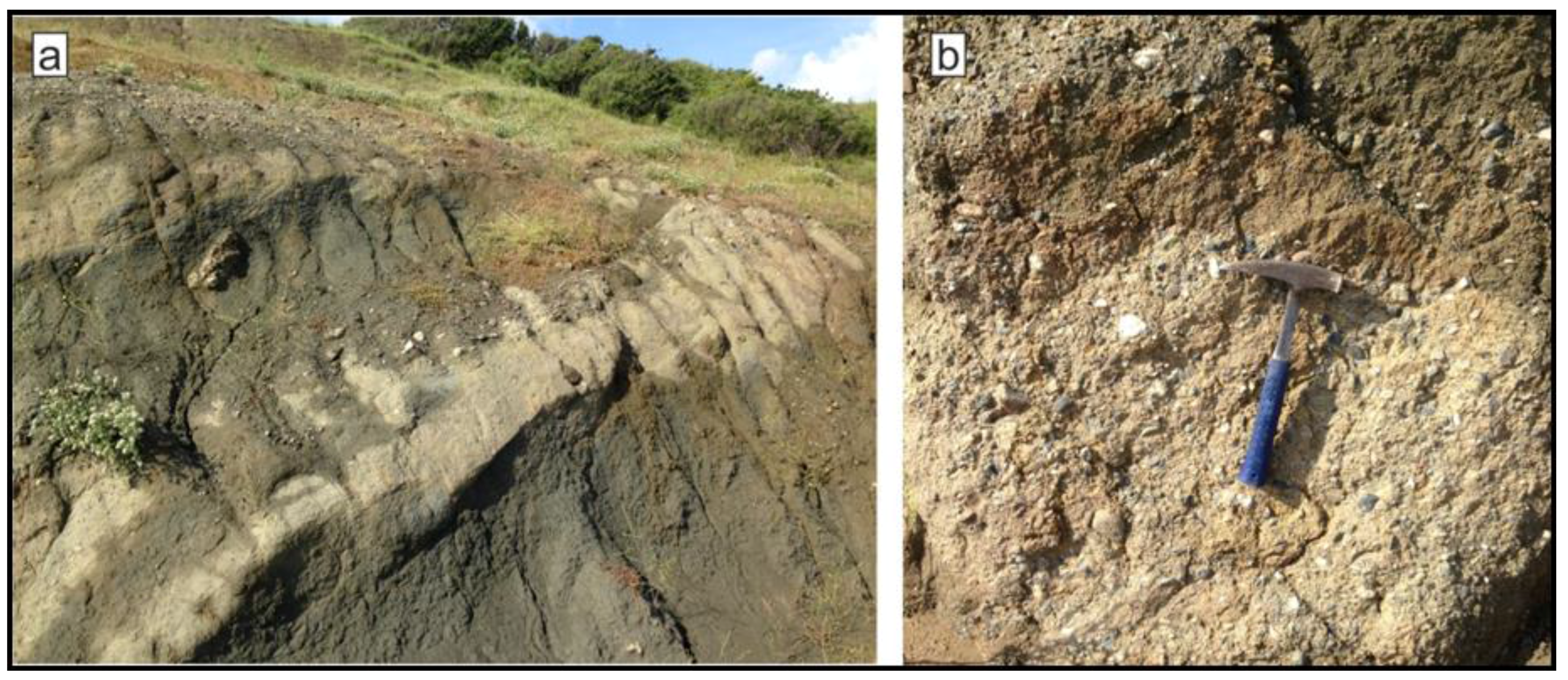
40]. The sandstones of the Fıçıtepe Formation are massive and strongly cemented. Conglomerate is seen as strengthen gray-beige and insubstantial when compared with the sandstones. Units of sandstone and conglomerate are observed as being interbedded (
Figure 3a). The dimensions of the conglomerates range between 1 cm and 15 cm (
Figure 3b). Large samples of some conglomerate are identified as they are mostly made up of parts of quartz and volcanic pebbles.
Figure 2.
The geological map of Sevketiye area (modified [
39]).
Figure 2.
The geological map of Sevketiye area (modified [
39]).
Figure 3.
(a) The sandstone and conglomerate of the Fıçıtepe Formation; and (b) lightly cemented conglomerate (UTM 488,541 m East, 4,471,678 m North).
Figure 3.
(a) The sandstone and conglomerate of the Fıçıtepe Formation; and (b) lightly cemented conglomerate (UTM 488,541 m East, 4,471,678 m North).
The region is mainly used for agricultural purposes by dwellers. However, unlike the surrounding stable areas, the landslide surface is largely covered by some valueless plants growing wildly and profusely. The study area has a transitional climate between a temperate Mediterranean climate and a temperate Oceanic climate, with warm to hot, moderately dry summers and cool to cold, wet winters. According to the Turkish State Meteorological Service (TSMS) [
41], temperature extremes in the study area range from 39.0 °C in July 2007 down to
−11.2 °C in February 2004. The average annual precipitation of the study area was 618 millimeters over the period 1981
–2014.
The landslides, which have frequently occurred alongside the highway in the area, have partly caused deformations in the road. Despite the fact that there have been no official reports about the landslides, which, according to the field observations, have occurred over the last two years, the landslides can be characterized as being slow moving. In terms of the scope of the research project indicated in the acknowledgments section, Erenoglu
et al. [
42] defined lateral and vertical electrical changes of the subsurface as characterizing the Şevketiye landslide. They used the electrical resistivity (ER) method in that it is considered to be a common and primary method used to investigate landslides [
43]. In the above-mentioned work [
42], nine profile tomography measurements were carried out with a minimum of 5 m electrode intervals and a maximum 75 m profile length. According to the geophysical surveys, the area is fairly shallow, with a high underground water level and water-saturated area, especially in the northern part of the area. Furthermore, while there are swellings and fallings from place to place, it is possible to observe surface cracks of different sizes opening up at the boundaries of the slope. Considering that the presence of water is an important factor, which triggers the movement of the landslide areas, it must be taken into account in order to seasonally monitor the saturated field units, showing the high conductivity of the area and the morphological changes [
42].
The Sevketiye region, which is located in the north-west of Marmara region, Canakkale, Turkey, is very close to the Saros extension of the North Anatolian Fault Zone (NAFZ), which is well known to be the most prominent active fault system. The Izmit earthquake on 17 August 1999 caused considerable loss of life and damage in the region. NAFZ is a major right-lateral, strike-slip, vertical fault, extending about 1200 km from the Karlıova Triple Junction (KTJ) in eastern Turkey to the northern Aegean Sea, accommodating the westward motion of the Anatolian plate relative to Eurasia [
42,
44,
45,
46].
3. Photogrammetric Process
The process used for this research was UAS, using a TurkUAV Octo XL microcomputer (
Figure 1b). The vehicle had eight engines and their propellers and could carry a payload of two kilograms; the 14.8 V 11,000 mAh LiPo battery provided flight duration of up to 18 minutes. The aerial images were taken by Canon EOS M 18.0 MP compact camera systems. As the single-lens reflex (SLR) cameras had mirrors, which were more sensitive to the vibrations, the EOS M compact system was chosen for the project.
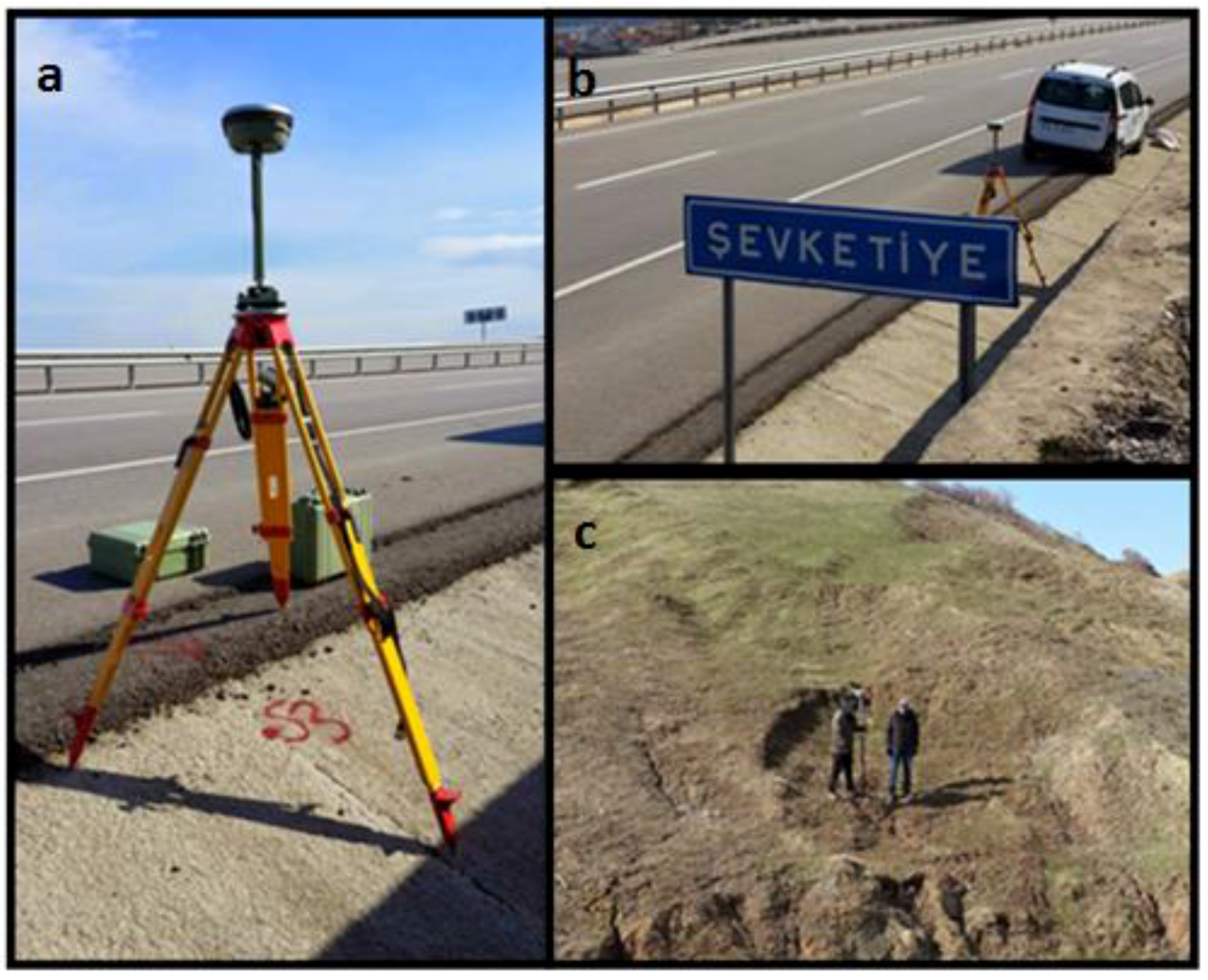
Twenty-one ground control points (GCPs) were permanently established around the landslide surface, and the coordinates of the GCPs were measured using two Global Navigation Satellite System (GNSS) receivers using the Real Time Kinematic (RTK) technique. The locations of the GCPs were deliberately picked to ensure as good a distribution across the study area as possible, for temporal monitoring of the landslide using both photogrammetric and geodetic methods in future survey campaigns. In
Figure 4, the left and the upper right images show the GNSS receiver on the base station, whereas the right lower image shows the rover receiver at the Sevketiye landslide.
Photogrammetry establishes the relationship between the image and the object using projective geometry. The calibration process of the digital camera and photogrammetric process were carried out using Photomodeler software [
6]. To specify the spatial position and orientation of the camera in the geodetic coordinate system, the exterior orientation is described by
acting as the coordinates of the perspective centers in the geodetic coordinate system and
being three suitably defined angles expressing the rotation of the image coordinate system with respect to the geodetic coordinate system. The exterior orientation of the images, which was denoted by
, were computed in the Photo Modeler Software using its SmartMatch (SM) feature. The SM capabilities of Photo Modeler include finding unique interest points in images of the scene and robustly matching them to corresponding points in images from different viewpoints [
47]. The main photogrammetric process algorithm was computed using the bundle adjustment [
48,
49,
50], which is also called fine-tuning after the 85,456 features that were detected automatically in the project. As a result of the bundle adjustment, the positions of the camera centers
, the rotation angles
, and the refined camera parameters were obtained [
51].
Figure 4.
(a) The base station Global Navigation Satellite System (GNSS) receiver; (b) The base station GNSS receiver from different view angle; (c) mobile GNSS receiver on the landslide surface.
Figure 4.
(a) The base station Global Navigation Satellite System (GNSS) receiver; (b) The base station GNSS receiver from different view angle; (c) mobile GNSS receiver on the landslide surface.
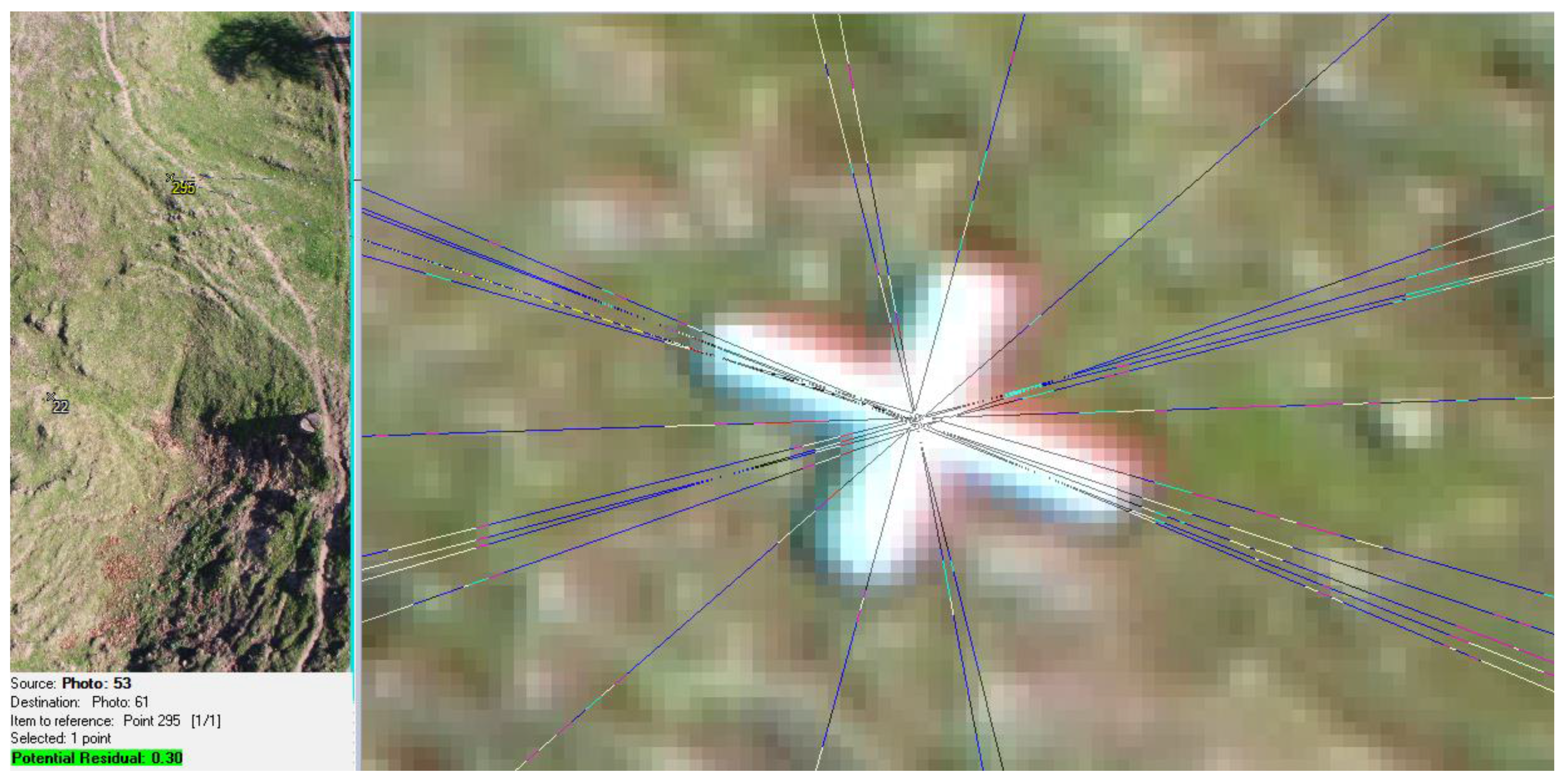
Afterwards, the image coordinates of the GCPs were measured on the photogrammetric model. In
Figure 5, a GCP is shown with epipolar lines, which help to check the marking precision of GCP. The figure also shows that the potential root mean square for the marking during the measurement was 0.30 pixels. The minimum RMS value was 0.001 pixels and the maximum RMS value was 2.921 pixels for the automatically detected and matched points. Besides this, the RMS values of the image coordinates of the GCPs varied from 0.086 to 2.293 pixels in the photogrammetric project, as seen in
Table 2. The coordinates of the GCPs, which had ±1cm accuracy, were used to define the seven-parameter Helmert coordinate transformation from the model coordinate system to the geodetic coordinate system.
In
Table 2, the results show that the vectorial magnitude of the differences between the GPS coordinates and photogrammetric coordinates varied from 15 mm to 122 mm.
After bundle block adjustment and the coordinate transformation were implemented, the geodetic coordinates of the projection centers of the cameras were obtained. The average value of the Z coordinate of the projection centers implied the average flight height of the UAS, which in the project, the average flight height of 132 photos was determined as 58 meters above sea level.
The 3D point clouds were produced using the Multi-View Stereo (MVS) technique [
52]. The technique takes the output from the bundle adjustment and performs a match to derive 3D dense point clouds [
53]. After the 3D geometry of the surface shape and the orientation parameters of the photos were solved, the orthophoto at 3 cm/pixel spatial resolution was produced. This is an orthographic projection of photographs with the perspective distortions removed, which was obtained for the landslide area (
Figure 1b) [
54].
Figure 5.
Epipolar lines predict the possible position for a ground control point (GCP) during marking.
Figure 5.
Epipolar lines predict the possible position for a ground control point (GCP) during marking.
Table 2.
Photogrammetric precisions of GCPs and differences of measurements between GPS and Photogrammetry.
Table 2.
Photogrammetric precisions of GCPs and differences of measurements between GPS and Photogrammetry.
| Point Id | RMS Residual (Pixels) | X Precision(m) | Y Precision (m) | Z Precision(m) | ΔX=XGPS −XPhoto (m) | ΔY=YGPS −YPhoto (m) | ΔZ=ZGPS −ZPhoto (m) |
|---|
| 1 | 0.821 | 0.005 | 0.003 | 0.009 | 0.078 | −0.020 | −0.007 |
| 22 | 0.826 | 0.002 | 0.002 | 0.005 | −0.039 | 0.071 | −0.035 |
| 41 | 1.244 | 0.004 | 0.003 | 0.009 | −0.019 | −0.041 | 0.005 |
| 50 | 2.293 | 0.003 | 0.002 | 0.006 | −0.002 | −0.024 | 0.005 |
| 55 | 0.548 | 0.003 | 0.002 | 0.005 | −0.050 | −0.023 | 0.004 |
| 73 | 1.607 | 0.003 | 0.002 | 0.006 | −0.001 | 0.013 | −0.042 |
| 92 | 1.620 | 0.003 | 0.002 | 0.005 | −0.003 | 0.038 | −0.037 |
| 111 | 1.614 | 0.003 | 0.002 | 0.005 | 0.012 | 0.059 | −0.039 |
| 126 | 2.027 | 0.002 | 0.002 | 0.005 | 0.045 | 0.062 | −0.095 |
| 143 | 1.370 | 0.003 | 0.002 | 0.007 | 0.020 | 0.026 | 0.005 |
| 158 | 0.995 | 0.004 | 0.003 | 0.008 | 0.021 | 0.014 | −0.030 |
| 193 | 1.949 | 0.002 | 0.002 | 0.004 | 0.031 | −0.006 | −0.028 |
| 217 | 1.260 | 0.003 | 0.003 | 0.008 | −0.014 | 0.038 | −0.035 |
| 240 | 1.584 | 0.002 | 0.002 | 0.006 | 0.022 | 0.017 | −0.005 |
| 247 | 1.654 | 0.002 | 0.002 | 0.005 | 0.021 | 0.039 | −0.037 |
| 267 | 1.403 | 0.003 | 0.002 | 0.005 | −0.027 | −0.063 | 0.020 |
| 283 | 0.849 | 0.004 | 0.003 | 0.008 | 0.030 | 0.037 | 0.015 |
| 292 | 1.733 | 0.003 | 0.002 | 0.005 | 0.006 | 0.009 | −0.010 |
| 295 | 0.630 | 0.003 | 0.002 | 0.005 | −0.065 | 0.052 | 0.012 |
| 306 | 0.521 | 0.003 | 0.003 | 0.007 | 0.029 | 0.064 | −0.085 |
| 316 | 1.332 | 0.005 | 0.004 | 0.009 | −0.008 | 0.089 | -0.028 |
4. Workflow for Machine Learning
Landslide susceptibility mapping predicts the spatial hazard that includes the location, volume or area, classification and velocity of the potential landslide, and any resultant detached material, and the probability of their occurrence within a given period of time [
55] by evaluating the related data selected from qualitative or quantitative parameters, such as the slope, curvature, lithology, soil type, land use, distance to faults, distance to roads, rainfall,
etc. These parameters are commonly considered as the factors associated with landslides for small to medium scale research. As Unmanned Aerial Systems (UAS) are capable of gathering high-resolution image data, landslides can now be explored in detail for larger scales. In this research, topographic features were considered as the main parameters related to landslides, whereas other variables, such as lithology, soil type, land use, distance to faults, distance to roads and rainfall were obsolete for the fields about 1 square kilometer, since the notable variations will not be expected in such narrow areas. In the proposed data modeling, three datasets, namely, slope, aspect, and visually uniform regions were studied to investigate the sufficiency of representative of linear fissure structures, which had occurred on the landslide surface. The other parameters such as the stream power index, the topographic wetness index and curvature were excluded from the proposed models, because the experiments discussed in the results section yielded insignificant changes statistically.
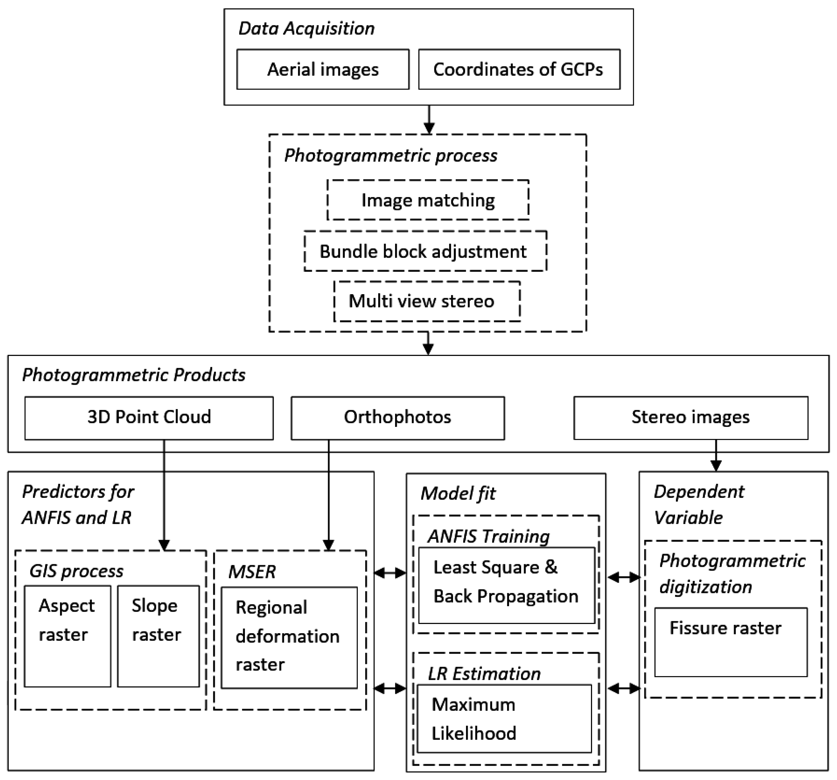
Figure 6 illustrates the whole workflow from data acquisition to data modeling, including the photogrammetric process and its products, and the model fit.
In this paper, both logistic regression having multiple explanatory variables [
56] and the first order Takagi–Sugeno neuro fuzzy inference system [
57] were implemented. The introduced machine learning model builders presented in the paper have three predictors,
, as shown in
Figure 6. The cell-based datasets represent topographic features, the aspect raster
, the slope raster
, and the raster represents regional deformations
, which are called the input layer (layer 1) for the ANFIS, while they are called the independent variables for LR. The dependent variable was the linear fissure structures that were produced from UAS photogrammetry.
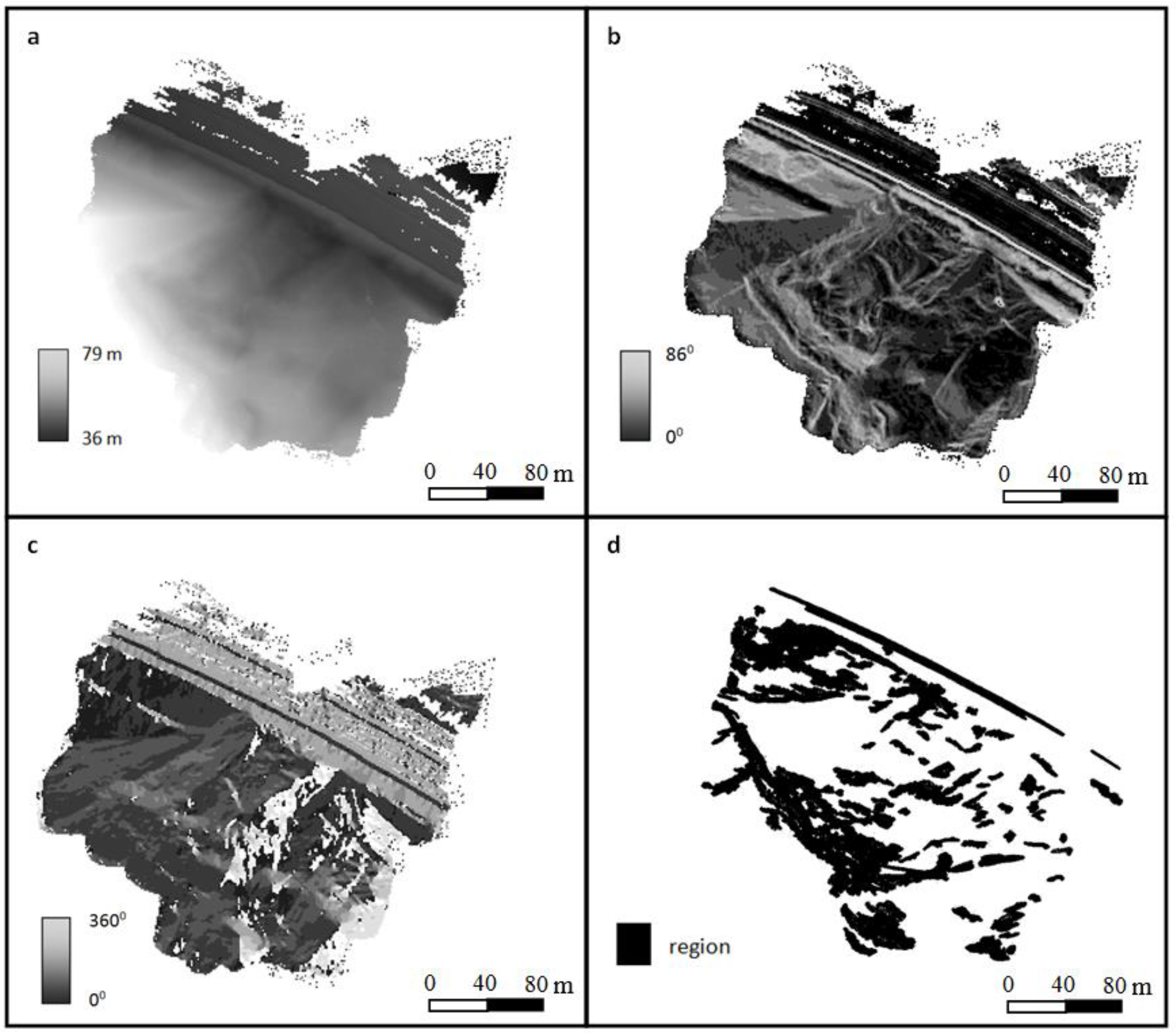
The three datasets that were mentioned in the preceding paragraphs are accepted as the predictors of the proposed ANFIS and LR. The aspect map and the slope map, as the two input variables of the model fittings, were obtained as rater datasets from the 3D point cloud of the landslide region, using the spatial analyst tools of the ARCGIS software. The point features of the photogrammetric point cloud were converted to the raster cells, whose values represented the height (Z) information. The arithmetical mean of Z values of all the corresponding points inside any cell was assigned to that cell as the elevation (
Figure 7a). Subsequently, the slope was determined as the rate of change of elevation for each elevation cell (
Figure 7b). Then, the aspect raster identified the downslope direction of the maximum rate of change in value from each cell to its neighbors (
Figure 7c).
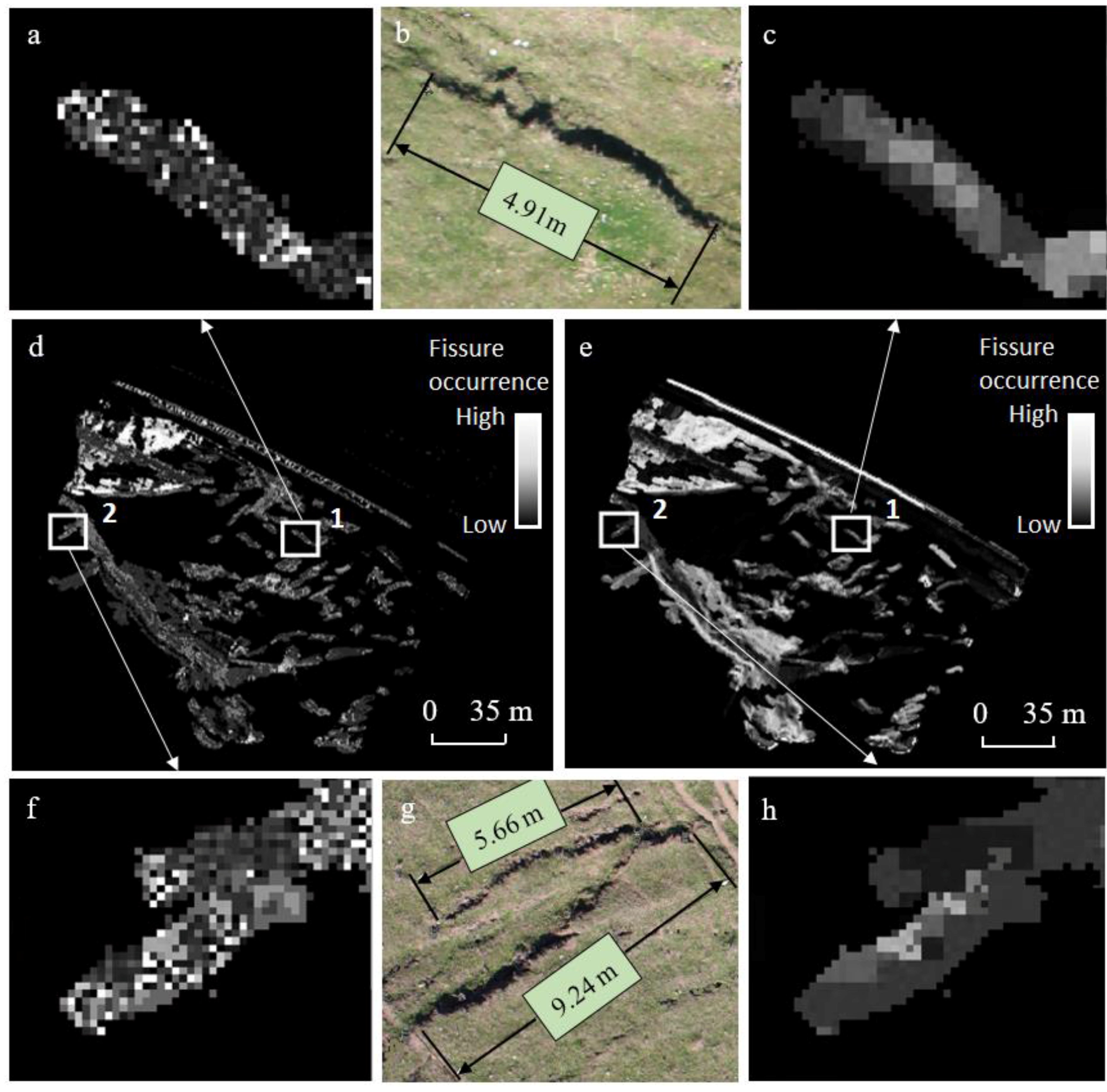
The third input variable, regional deformations, was automatically estimated using the maximally stable external regions (MSER) algorithm [
58]. The regions were defined solely by the external property of the intensity function in the region and on its outer boundary. The fractures that occurred on the landslide surface caused naturally regional traces on the orthophotos, which were produced. As the regional traces on the orthophotos occurred mostly due to the fractions, MSER considerably indicated the fissure presence. The percentage of the MSER regions, including a pixel belonging to a fissure and its eight-neighborhood was sixty-one percent when a cell-based comparison was carried out between the MSER image and the digitized fissure features of the stereo images (
Figure 7d).
Figure 6.
Data processing flow.
Figure 6.
Data processing flow.
The fissure features, which represented the dependent variable of LR, were also called the output variable of ANFIS, were obtained from the stereo images of the landslide surface. Twenty-eight different profiles that deliberately intersected explicit fissure structures were randomly determined around the landslide area. Only 10 of the 28 profiles are depicted in
Figure 8 for the sake of simplicity. The lower values of the gray-scale orthophotos correspond to the fissure structure and contrast sharply with their brighter neighborhoods, as seen in all the profiles.
In this section, the relationship among input variables is discussed. The cell-based values of slope, aspect, MSER regions and orthophotos along profile 6, are depicted in
Figure 9; all graphics were normalized by scaling them between 0 and 1 to relate the different variables properly. The lowest value of the orthophotos of a profile is indicated as the dashed red line as seen in
Figure 9, as the lower grey values of the orthophotos profoundly imply fissure structures. In the first row of
Figure 9, the slope cells clearly show the profiles that were reached at the angle of high degrees across the fissure.
The second row of
Figure 9 shows that the aspect values of the profiles mostly stand around 0 or 1. The minimum and maximum values, 0 and 1, that are normalized from the aspect raster having 0–360 degree range, represent the north direction. As the northeast was the main movement direction of the landslide, the profiles are around 0 at the fissure structure. On the other hand, MSER regions were considered as the third input variable in order to distinguish fissure intensive regions from intact fields. The MSER figures apparently depict that darker grey values were associated with MSER regions.
Figure 7.
(a) Elevation raster; (b) slope raster; (c) aspect raster; and (d) Maximally stable external regions (MSER).
Figure 7.
(a) Elevation raster; (b) slope raster; (c) aspect raster; and (d) Maximally stable external regions (MSER).
In addition to the inspection of the profiles, the histograms of the square region that surrounds profile 6 in
Figure 9 were also considered for each input. In
Figure 9, the histogram of the slope, which had five separate groups of occurrence, indicates the high slope values at the fifth group around 0.75. The histogram of the aspect intensified around the values of 0.2 and 0.3. Particularly fissures, which were distinguished in the aspect raster as the fissure related areas befit aspect values around 0.2. MSER regions, which are depicted as darker values, are accumulated around the 0 value. In the orthophotos, the image fissure area appeared as a black region, therefore, the histogram of the orthophotos shows a tiny aggregation between the values of 0 and 0.2. Despite this, there is no exact coincidence observed between the orthophotos and the input rasters; the occurrence of some distinctions on the input rasters are observed around the fissure area.
Figure 8.
Showing some profiles that intersected the fractures around the landslide surface.
Figure 8.
Showing some profiles that intersected the fractures around the landslide surface.
Table 3 shows the classes of each input data layer, the number of pixels of the classes, and the number of fissure occurrences belonging to the classes. The classes were used for the implementation of the ANFIS and LR models. Both the aspect input and MSER inputs were clustered into two classes, as attributes 1 and 2, while the slopes were considered as continuous data between intervals 0–1.00. Despite this, the aspect had nine faces (flat, northeast, east, southeast, south, southwest, west, and northwest).
The mean value of the aspect data of the training dataset where the fissures occurred was calculated as 48.26 degrees, indicating that the northeast was approximately the direction of the main movement of the landslide. Moreover the pixel values that did not encounter a fissure structure were observed in a homogenous distribution in all directions except northeast. Therefore, the first category of the aspect was recognized as between 0 and 90 degrees, while the other directions (between 90 and 360 degrees) were accepted as the second category. On the other hand, MSER data in the training dataset accumulated into two opposite centers in that the first center was zero and the second center was one. For this reason, all pixels that were below the 0.5 value were defined as a region from the MSER region raster, while other pixels (>0.5) were grouped into the attribute 2 of MSER.
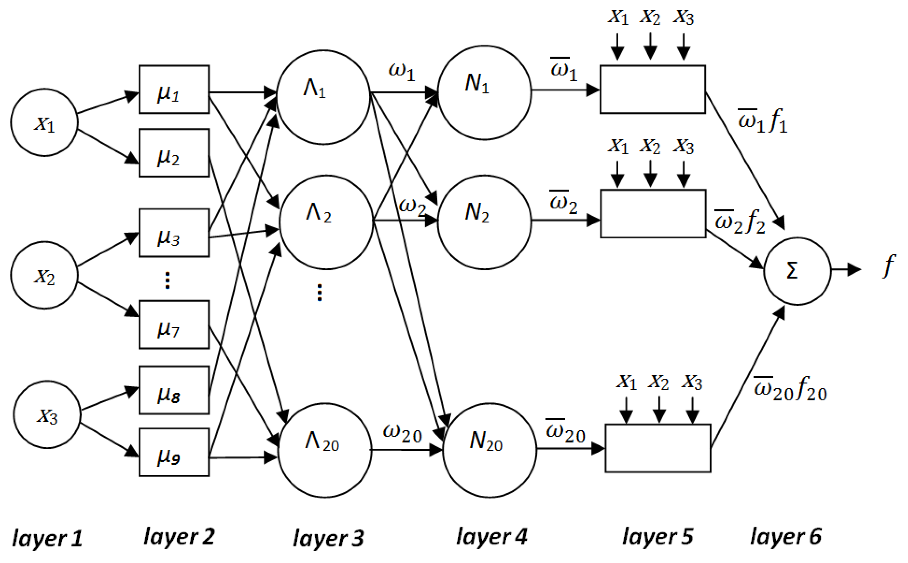
4.1. Adaptive Neuro Fuzzy Modeling: ANFIS Analysis
Using a given input/output dataset, the ANFIS constructed a fuzzy inference system (FIS), whose membership function parameters were tuned using a back propagation algorithm, in combination with a least squares type of method. As shown in
Figure 10, the attributes of the adaptive neuro fuzzy inference system, which was applied for the mentioned inputs and outputs, is explained in detail in the preceding section. An initial fuzzy inference structure was determined in the fuzzification layer (layer 2) of the ANFIS. In order to represent all the data within a moderate number of rules, two generalized bell-shaped membership functions (also known as the Cauchy membership function) using Equation (1), had been assigned to the aspect and MSER input datasets and five generalized bell-shaped membership functions had been assigned to the slope input dataset, as seen in
Table 4. While a linear membership function had been assigned to the output data using the grid partition method. In Equation (1),
µ(
x) indicates the generalized bell-shaped membership function, while the parameter
c defines the center of the curve and the parameters
a and
b define the width of the curve.
Figure 9.
Showing the profiles that intersected the fractures around the landslide surface.
Figure 9.
Showing the profiles that intersected the fractures around the landslide surface.
Table 3.
The summary of input data layers.
Table 3.
The summary of input data layers.
| Input Data Layers | Layer Classes | Normalized Layer Classes | Pixels In Classes | Fissure Pixels | Attributes |
|---|
| Aspect | 0–90 | 0–0.25 | 588 | 384 | 1 |
| | 90–360 | 0.25–1.00 | 326 | 34 | 2 |
| Slope | 0–86 | 0–1.00 | Continuous | Continuous | 0–1.00 |
| MSER | 0–0.50 | 0–0.50 | 680 | 406 | 1 |
| | 0.50–1.00 | 0.50–1.00 | 234 | 12 | 2 |
Figure 10.
The proposed Adaptive Neuro Fuzzy Inference System (ANFIS) network.
Figure 10.
The proposed Adaptive Neuro Fuzzy Inference System (ANFIS) network.
Table 4.
Membership functions for input data layers.
Table 4.
Membership functions for input data layers.
| Input Data Layers | Membership Functions | Function Type |
|---|
| Aspect | | Generalized bell shaped |
| Slope | | Generalized bell shaped |
| MSER | | Generalized bell shaped |
Table 5.
The summary of the proposed ANFIS.
Table 5.
The summary of the proposed ANFIS.
| Layer No | Layer Type | Number of Nodes | Number of Parameters |
|---|
| 1 | inputs | 3 | 0 |
| 2 | fuzzification | 9 | 27 (non-linear) |
| 3 | rule antecedent | 20 | 0 |
| 4 | normalization | 20 | 0 |
| 5 | rule consequent | 20 | 80 (linear) |
| 6 | inference | 1 | 0 |
| | Σ | 73 | 107 |
The antecedent part of the rules, also known as fuzzy combinations, was calculated in layer 3 using the product t-norm (triangular norm) (Equations (2)–(4)). Twenty output nodes, which represent the firing strength of the corresponding fuzzy rules, were obtained. In layer 4, each node calculates the ratio of the i-th rule's firing strength to the sum of all rules firing strength, which is also called the rule strength normalization, as described in Equation (5). Layer 5, as the consequent rule layer, shows every output node of layer 4 with the node function and p, q, r and s are the parameters of the node function as indicated in Equation (6). Eighty linear parameters of consequent rule can be determined using the least square algorithm. In the rule inference layer (layer 6), as written in Equation (7), the single overall output node was computed as the summation of all nodes coming from layer 5. The properties of the proposed ANFIS model are summarized in
Table 5.
Three subgroups in the fissure areas were obtained separately in the form of training, test, and check datasets from the corresponding cells of images of the inputs and the output. Each training dataset for ANFIS included a 914 input-output combination, which was several times larger than the total number of parameters (107 being estimated). The ANFIS learning updates membership function parameters with the hybrid algorithm method consisted of back propagation for the input membership function parameters and least-square adjustment for the linear function parameters. In the forward pass, non-linear parameters were fixed and linear function parameters were computed using least square, in the backward pass, linear function parameters were fixed and non-linear parameters were computed using back propagation.
Table 6 explains the results of RMSE (Equation (8)) and the coefficient of determination. This was also known as R-squared (Equation (9)) at the end of 35 training epochs of ANFIS learning. In this research, ANFIS analyses were performed using the MATLAB programming software.
Table 6.
The summary of the statistical criteria of RMSE and R2 of the ANFIS model.
Table 6.
The summary of the statistical criteria of RMSE and R2 of the ANFIS model.
| Data Type | Epoch | RMSE | R2 |
|---|
| Training | 35 | 0.0218 | 0.9990 |
| Check | 35 | 0.0643 | 0.9914 |
| Test | 35 | 0.0868 | 0.9846 |
4.2. Statistical Model: Logistic Regression Analysis
Logistic regression, also called a logit model, was used to model dichotomous outcome variables. In the logit model, the log odds of the outcome were modeled as a linear combination of the predictor variables (Equation (10)). In Equation (10),
indicates intercept, while
represents three coefficients of predictor variables. The predictor variables
were used, as defined in the same order, which are given in
Table 3. Maximum Likelihood (ML) is a way of finding the smallest possible deviance between the observed and predicted values, specifically using derivatives y. In this research, the event occurrence was represented by the presence of fissures within a pixel and the logistic regression was exploited to predict a binary variable that could be equal to 1 (presence of fissure) or 0 (absence of fissure). In this study, logistic regression analyses were performed with statistical software R [
59], enabling categorical explanatory variable definition.
The fit of the regression model with data observed from the training datasets of profiles was quantitatively evaluated by the null deviance
, the model deviance
, chi-square
and
pseudo-R2 statistics. The null deviance
was calculated as 630.20, by comparing the null model with the theoretical model (also known as the saturated model), the model deviance
was calculated as 340.57 by comparing the full model, including all predictors with the theoretical model, while chi-square
was determined as 289.63 using Equation (11). The set of predictors significantly improved the model fit that can, therefore, be concluded from the regression results, as the model deviance is significantly smaller than the null deviance. The models fitting to the observed data can also be evaluated by three different
pseudo-R2 computing variables, instead of adjusted R-squares in the case of a multiple linear regression model, in addition to the statistic
. Results of the
pseudo-R2 of McFadden, Cox and Snell, and Nagelkerke were obtained as 0.4596, 0.4694, and 0.6274, respectively. The values around 0.5 of these
Pseudo-R2 parameters indicate a statistically significant fit of the logit model with the training data.
Table 7 explains the coefficients obtained, the Wald test results, and the
p-values for the predictors after the logistic regression was implemented. According to
Table 7, the slope coefficient shows that for every 1 unit increase in slope value, the logit of the probability of a fissure occurrence increased by 6.1726. Since the all
p-values are quite small, the predictor variables explained a significant amount of the deviance.
Table 7.
coefficients, Wald test and p-values for the predictors.
Table 7.
coefficients, Wald test and p-values for the predictors.
| Predictor | Coefficients | Wald Test | p-Value |
|---|
| Intercept | −1.5739 | −4.461 | 0.0000 |
| Aspect | −1.2875 | −3.717 | 0.0002 |
| Slope | 6.1726 | 7.361 | 0.0000 |
| MSER | −4.1768 | −4.076 | 0.0000 |
6. Conclusion Remarks
In the proposed workflow, UAS is critically important to collect high-resolution data, whereas an aerial camera on a plane makes missions expensive. Moreover, a commercial photogrammetric aerial camera provides images of 5 cm GSD at most, due to its flight height. UAS, which has the advantage of low altitude flight, is an inexpensive technology when compared to aerial monitoring with an airplane and provides images under 1 cm GSD. The XYZ precisions of all GCPs measured on the UAS images were under 1-cm accuracy, as seen in
Table 2. The comparison between the GPS measurements and photogrammetric measurements also reveals satisfying results. The mean values of the absolute differences between the two measurements were 26 mm in X direction, 38 mm in Y direction and 28 mm in Z direction. The coordinate differences might have occurred with the accumulation of many sources of error, such as RTK measurement errors, photogrammetric measurement errors, errors during GCP target placement on the ground and coordinate transformation errors. The results clearly show that UAS photogrammetry is a convenient technique for monitoring landslides and their expected periodical changes over 5 cm.
The high-resolution, cell-based geo-referenced datasets have considerable potential for landslide modeling. This is particularly true for photogrammetry, which is able to produce fast and accurate datasets showing where fissures have occurred on the landslide surface, which are strongly related to the elevation, the aspect and the slope. The weight of the topographic features at the fissure modeling of the landslide area has been considered in this research. However, the topographic features are not enough input variables to detect fissures. A visual restriction, or a visual supporter variable like the MSER region algorithm, as used in this work, provides a contribution to the data model. The MSER regions, as a region extraction algorithm, also added to the ANFIS and LR inputs, in order to confine the data model on fissure relevant locals.
However, during the ANFIS and LR modeling, the major challenge was to determine a convenient training and test output dataset that represented the fissures. To provide full automation, high-resolution orthophotos can be used as an alternative fissure extraction for the training and test data. The advantage of the full automatic process of the fissure extraction, which was due to grey value change showing fissure structure, can be considered as a useful tool among the fissure modeling methods. The results of all datasets, training data, check data and test data indicated moderate errors, despite the datasets, which might include some blunder errors when the randomly produced profiles from raster datasets are examined.
As the orthophoto is a key dataset necessary to produce MSER data, its resolution is directly involved with the ANFIS and LR training performance. The higher resolution the orthophoto is means the more accurate the cell-based datasets are to use in ANFIS as the variable. The higher the resolution of the orthophoto, however, means the computing tasks are more complicated due to the intensive data, which might cause problems during the implementation in ANFIS and LR models. In the future work, depending on the different resolutions, ANFIS performance and results should be discussed deliberately.
The new ANFIS and LR data modeling, which is an extent of the proposed model, will also be applied with the next process of photogrammetric data acquisitions in order to interpret landslide changes. The relation between the automatic recognition of the changes on the landslide surface and the DEM data and its derivatives will be probably explained with reasonable data modeling. In this research, grey-scale images were preferred because the data intensity was too much to process in the cell-based application. The potential of RGB color images will probably produce better results than the grey-scale images.
During the extraction of the fissure occurrences using the either the ANFIS or the LR models, the sensitivity of MSER region algorithm about shadowing effects influenced inferences negatively. As the natural and artificial objects, such as trees and buildings might cause an increase in inaccurate output cells, the proposed models are recommended for use in bare fields or places having rare vegetation and settlements, for a successful automatic implementation, so as to obtain more precise results.


