1. Introduction
Most geographical phenomena have different characteristics at different scales in spatio-temporal domain. Various influences caused by many different factors simultaneously acting across scales lead the data on the phenomena to contain a mixture of multi-scale signals. The mixture of the multi-scale characteristics affects the data characteristics in both spatial and temporal domains. In the spatial domain, the characteristics of a given phenomenon should be represented with certain spatial range or resolution to support the complex remote sensing analysis including the object extraction, image segmentation, change detection, object tracking, and geostatistical analysis,
etc. [
1,
2]. In the temporal domain, the multi-scale characteristics of the data are acting as periodical or quasi-periodical signal at frequency ranging from hours to several decades. The effects of the multi-scale characteristics have attracted much attention, have been discussed in many different disciplines,
etc. [
3,
4,
5,
6].
Remote sensing data have been quickly accumulated continuously. More and more long-term remote sensing sequences (e.g., satellite and aerial images, SAR,
etc. [
7]), which cross the time span of more than several decades, are logged and used in various fields. These long-term data observations provide valuable information for detailed revelation of the evolution of the geographical processes [
8]. Along with the wide application of multi-temporal remote sensing data in many different fields, researchers have also proposed several different kinds of advanced analysis methods for feature extraction, segmentation,
etc. [
9].
There have already been some techniques proposed to solve these problems. Multidimensional data modeling and databases [
10,
11] and Array Databases (e.g., rasdaman [
12], SciDB [
13]) have largely improved the performance of storing and querying of the massive multidimensional spatio-temporal data. MOLAP (Multidimensional On Line Analysis Process), commonly used in data warehouse, is rapidly improved for multidimensional data queries and aggregation [
14]. Technologies, such as wavelets and hierarchical clustering of data are introduced to MOLAP to partly support the computation [
15,
16]. However, these analyses require accessing directly the most detailed data since no prior knowledge for the query exists. The spatio-temporal unified approaches (e.g., STIM [
17], Clifford Algebra/Tensor approaches [
18,
19]) are also proposed for the unified analysis of such huge amount of spatio-temporal data. However, these approaches are still in an early stage and too complex to be used directly in the operational environment.
Despite the large progresses achieved in the developing of multi-temporal remote sensing analysis methods, two critical problems still exist: (1) Most of these methods treat spatial and temporal dimensions separately. Several approaches can do multi-scale analysis in either spatial or temporal domain (e.g., EMD, wavelet, and parallel adaptive kernel smoothing) [
20,
21,
22]. Few methods can support for the spatio-temporal domain analysis in the spatio-temporal unified way [
23,
24]. With the separation of spatial and temporal signal in data analysis the spatio-temporal data can only be analyzed either spatially or temporally, which will lead to information missing, pattern inconsistency, and synchronizing difficulties. (2) Rarely methods integrate the multi-scale information during the exploratory data analysis. Although there are several exploratory data analysis methods, which can well reveal certain characteristics (e.g., value distributions, spectrum characteristics, and feature variations), developed, large percent of these methods are only applied to the overall data rather than the features at each scale. It is still complicated to reveal the multi-scale characteristics from different perspectives and perform the exploratory multi-scale spatio-temporal feature extraction.
Feature clustering, one of the most typical and commonly used exploratory analysis methods for multi-temporal remote sensing data, is largely restricted by the two problems mentioned above. Integrating multi-scale information in feature clustering can produce rich information about the spatio-temporal process and increase the feature clustering performance for feature extraction and process investigation. For example, various signals, including ocean currents and tides, high frequency variations (e.g., Madden-Julian Oscillation (MJO)), inter-decade variations (e.g., El Niño-Southern Oscillation (ENSO)),
etc. can be separated from the global ocean data according to their multi-scale characteristics differences [
25,
26]. With the multi-scale cluster in the spatio-temporal domain, the spatio-temporal evolution characteristics and processes of the above various signals can be revealed.
A fine performance multi-scale spatio-temporal feature clustering method should satisfy the following demands: (1) Since most geographical processes change continuously in the spatio-temporal domain, the analysis should be performed in the spatio-temporal domain with the consideration of the data continuity. (2) The feature clustering should be applied to components of different scales, which have different data distributions and different noise levels. Thus the feature clustering is better to be data adaptive and flexible. (3) Since the data volume of the original multi-temporal remote sensing data is usually large, and the multi-scale decomposition increases the data volume significantly, the feature clustering should be efficient for real world operational analysis. To achieve all the above requirements, new approaches should be developed to perform the multi-scale spatio-temporal feature clustering analysis.
This paper presents an integrated approach to perform the multi-scale spatio-temporal exploratory feature clustering. The paper is organized as follows:
Section 2 presents the overall idea of the proposed method.
Section 3 provides the details of the method. The case study with the satellite altimeter data is shown in
Section 4. The technical and geographical effectiveness of the method is evaluated in
Section 5. Discussions and conclusions are presented in
Section 6 and
Section 7, respectively.
2. Overall Idea
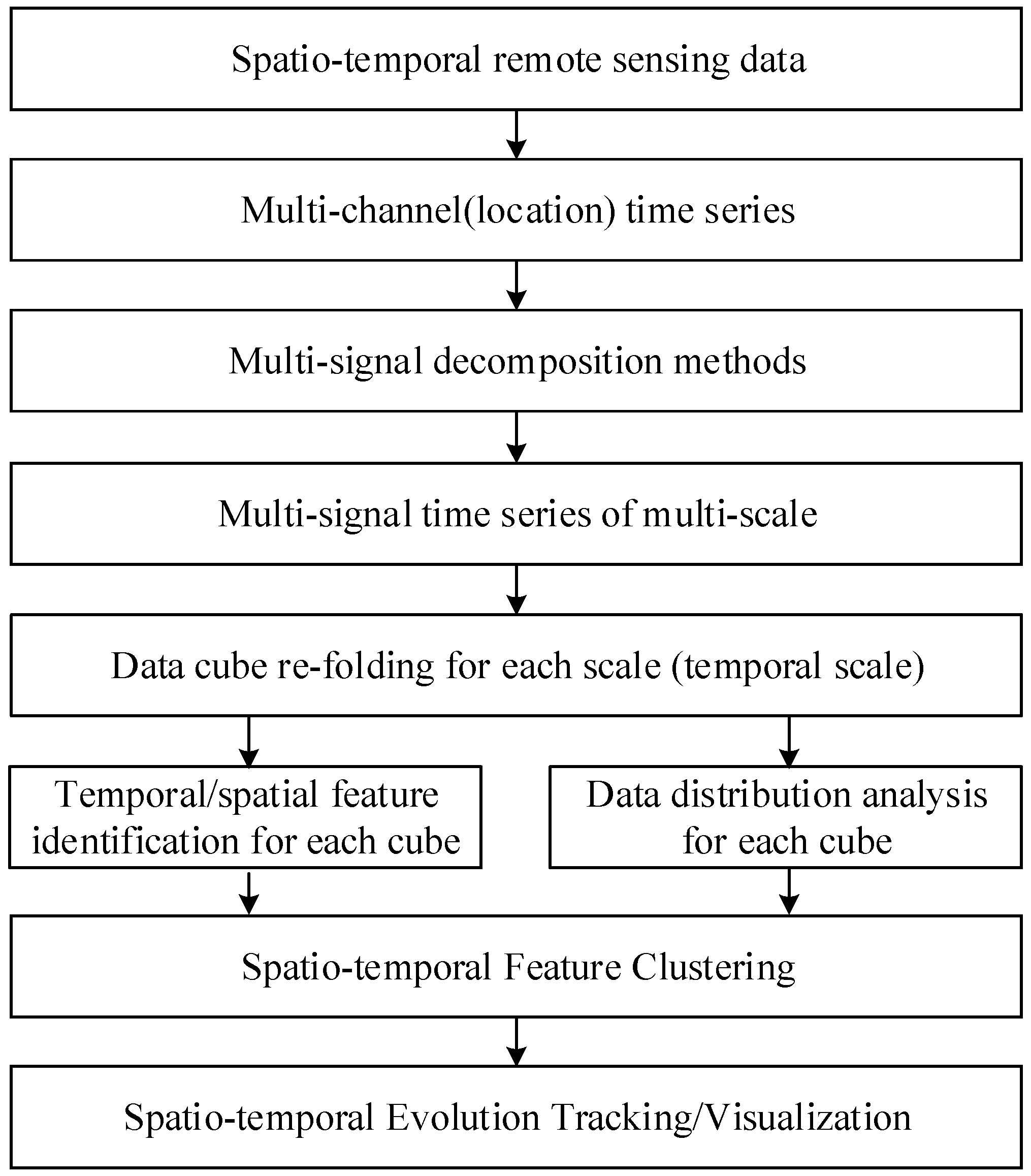
The overall idea of the exploratory multi-scale spatio-temporal feature clustering of multi-temporal remote sensing data is depicted in
Figure 1.
From the unified spatio-temporal perspective, the original multi-temporal remote sensing data can be considered as a unified spatio-temporal data cube. In this data cube, each location (pixels with same spatial coordinates) is a sampling with a time series indicating the temporal fluctuations through the temporal dimensions. Due to the lack of spatio-temporal unified multi-scale decomposition methods, the spatio-temporal multi-scale decomposition can only be performed in the spatial domain or the temporal domain. Therefore, the original spatio-temporal data, which are considered as a unified spatio-temporal data cube, should be unfolded as a multi-channel time series or spatial series. Under this notion, the entire multi-temporal remote sensing data over an area can be perceived as a set of time series with each location being a channel of time series. Therefore, the whole spatio-temporal data can be seen as a single multi-signal time series that is continuously observed at a synchronized temporal sampling rate. The spatial distributions of the data are inherited in the channel-to-channel relations.
Figure 1.
The overall framework of the exploratory multi-scale spatio-temporal feature clustering.
Figure 1.
The overall framework of the exploratory multi-scale spatio-temporal feature clustering.
Multivariate multi-scale analysis methods, such as multi-signal wavelet, can be applied to the multi-signal time series to extract the multi-scale variation patterns. The multi-signal wavelet decomposition estimates the common multi-scale variation pattern of all channels synchronically using the full information of the spatio-temporal data. Both global and the local spatio-temporal variations at different spatio-temporal scales can be extracted synchronically [
27]. With the multi-signal wavelet decomposition, the original multi-temporal remote sensing data can be decomposed into several multi-scale components. Each decomposed component, which is a multi-signal time series that indicates a certain feature of the multi-scale spatio-temporal variations, can be re-folded to a data cube with the same size of original data. Therefore, the connotative signals that only affect at certain significant scales can be extracted and revealed.
To enhance the feature extraction performance and filter out possible uncertainties or pseudo-variations caused by scale mixture or noise, classical exploratory data analysis methods, such as principal components analysis, power spectrum analysis and histograms, can be used to characterize the spatial/temporal features (e.g., spatial shapes or temporal indexes) and the data value distributions of the multi-scale variations. This can be achieved by comparing the features extracted by principal components analysis and power spectrum analysis with existing geographical indexes or spatial patterns to reveal geographical meanings of the multi-scale components. To identify the spatio-temporal distribution characteristics of the geographical phenomena, feature cluster methods such as K-Means, Fuzzy C-Means Cluster (FCM), etc., can be applied to the spatial/temporal histograms to achieve the spatio-temporal feature clustering. To achieve the data adaptive clustering for each decomposed multi-scale component, data indexes, such as entropy, can be used to develop the data adaptive optimized cluster number selection procedure. To improve the computational performance, the histograms can be used for feature clustering. The histogram-based cluster of the decomposed components helps to enhance the features of the data, which makes the data more separable. Since the data value distributions in the histogram bins are interlinked with different regions of data in the spatio-temporal domain, the original spatio-temporal data can be clustered by separating the histogram with the value distribution corresponding to the desired regions. With the clustered features, the evolution of the features can be tracked and visualized crossing different time stamps.
3. Methods
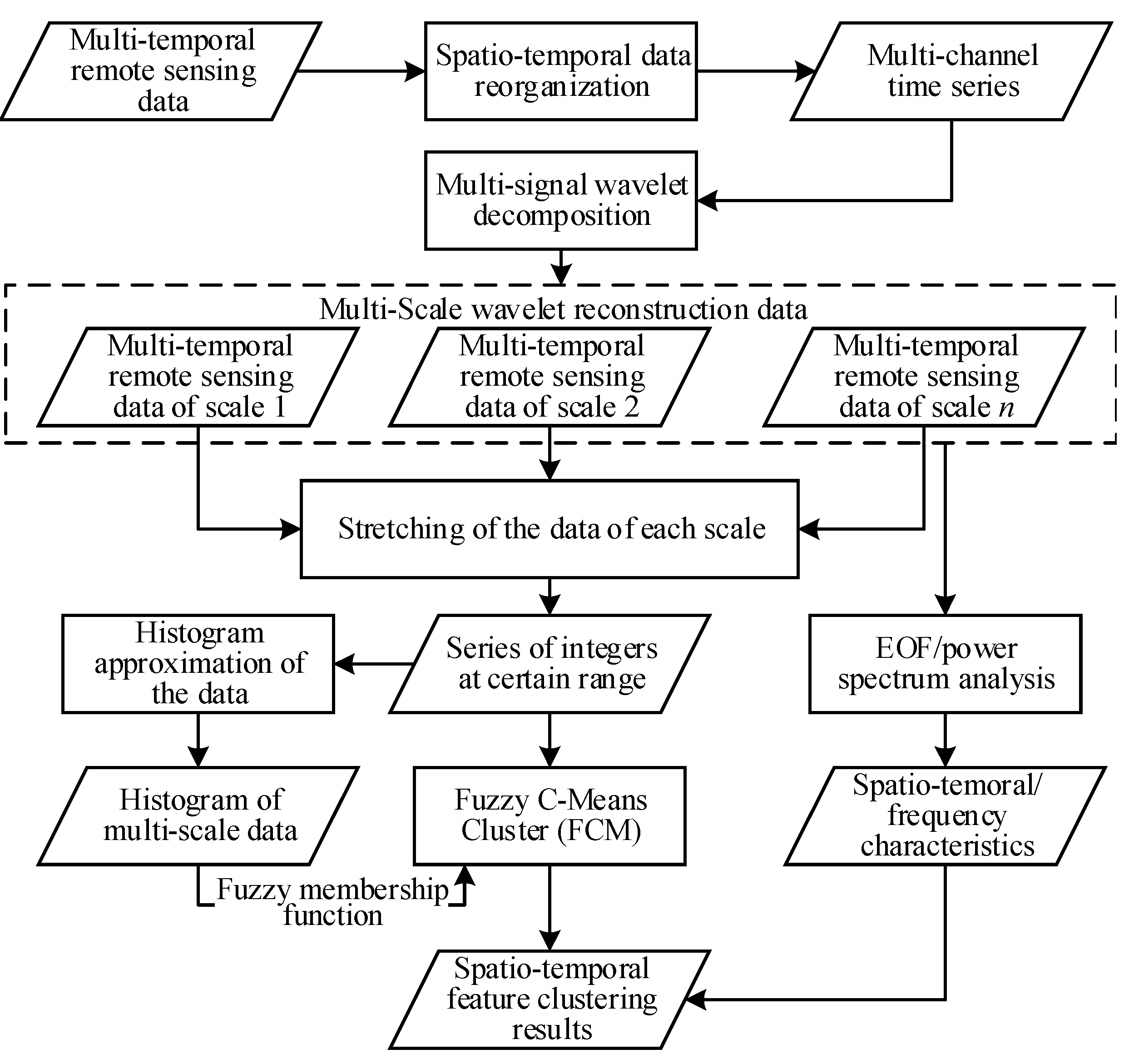
According to the overall framework, several methods are assembled and steadily integrated in a processing workflow (
Figure 2). The original spatio-temporal data are firstly reorganized as a multi-signal time series, which is then decomposed into several feature series cube and a noise cube by the multi-signal wavelet decomposition. The empirical orthogonal function analysis (EOF) and power spectrum analysis are applied to extract the spatio-temporal and frequency characteristics of each decomposed component. The integer approximation, which stretches the data, is used to enhance the data feature and reduce the computational cost. By reordering the data of integer approximation of each feature series cube in an ascend order and splitting them into several data bins, the histogram approximations can be constructed. Then the Fuzzy C-Means Cluster (FCM), with adaptively selection of cluster numbers, is applied to the stretched feature cubes. The segmentations of histograms are then reversely mapped to the spatio-temporal domain to achieve the spatio-temporal segmentation of original multi-temporal remote sensing data.
Figure 2.
The processing workflow.
Figure 2.
The processing workflow.
3.1. Spatio-Temporal Data Reorganization
In the beginning, we organize the multi-temporal remote sensing data as a unified multidimensional data cube [
28]. The unfolding is then applied to the data cube to form the multi-signal time series. Since there are usually more than one coordinates in the spatial domain, unfolding the original data cube into a set of time series with each spatial coordinates a time series (
i.e., spatial unfolding) will make the data much simpler. Therefore, we reorganize original data as unified spatio-temporal cube and then apply spatial unfolding to form the multi-signal time series. Although, the unfolding process of the original spatio-temporal data into the multi-channel signal appears to separate the spatial and temporal dimensions, the pattern extraction is done through the spatio-temporal distribution of the data and the data synchronization problems are naturally solved during the analysis.
3.2. Multi-Signal Wavelet Decomposition
Multi-signal wavelet decomposition is applied to the reorganized multi-signal time series to retrieval the multi-scale spatio-temporal variations. Assuming
X(
t)
= {
x1(
t),
x2(
t), …,
xM(
t)} is the
M dimensional multi-signal time series unfolded from the multi-temporal remote sensing data, the multi-signal wavelet decomposition of
X(
t) can be formulated as follows:
where
Fk(
t) is the deterministic feature series signal that has certain spatio-temporal scale characteristics,
ԑ(
t) is the spatial correlated residuals, which can be seen as noise, and
k is the level of features extracted.
Let
be the scale function.
M − 1 wavelet functions (notated as
j(i)(
t)) can be constructed. For each of the wavelet function that meet:
where
g(i) is the coefficient function of the wavelet filter of wavelet function
j(i)(
t).
Rapid algorithm [
29], which is constructed by parameterization of the mother wavelet and decomposition of the signal in the feature space, is used here for efficient decomposition. For each channel of the multi-signal, irrelevant elements involved in the signals are eliminated by a dyadic decimation, which reduces the original resolution into half of its length. This procedure is recursively applied on approximation coefficients to produce increasingly smoother versions of the original signals. Thus, we have the following decomposition:
where
is the approximation coefficient of the first scale,
is the approximation coefficients of the k-th scale,
is the detailed coefficient of the (
k + 1)-th scale, and
g(i) is the high pass filter of the scale function. Since the original data
X are a signal that have total
M channels, all the approximation coefficients
is a
M ×
pk matrix, where
pk is the same length as the DWT approximation coefficients at the
k-th scale.
The reconstruction of the multi-signal wavelet decomposition can be adopted in wavelet synthesis by up-sampling and inverse filtering of the decomposed coefficients. That is:
According to Equation (4), the approximation component at level j can be reconstructed with the approximation and detail components at level j + 1.
Since all the time series are decomposed at the same time, they are at the same time scales. As the decomposed components have the same size of the original data, exploring methods, such as principle components, histograms and power spectrums, can be direct applied to identify the characteristics and geographical meaning of these spatio-temporal variations at each scale.
3.3. The Stretching of the Data
To enhance the feature pattern of each decomposed component and reduce the computational cost, the data are stretched to the range that best represents its features. A simple mechanism, integer approximation, which projects float point data into a series of integers at certain range, is used. Given a multi-signal time series
, which has a value range (
a, b),
i.e.,
, where
a and
b are float values. The mapping of the multi-signal time series
X(
t) to the integer approximation in the range of (
m, n) can be formulated as follows:
where ℝ is the real number set,
is the value range of the series
X(
t), and the
is the positive integer set with the value range of (
m, n). A typical solution of the mapping is:
where (
x) is the function which aims at finding the closest integer of real value
x.
For each decomposed feature series cube, we can apply Equation (6) to project the whole data from the original value range (a, b) into the new value range (m, n) with their spatial and temporal distribution rarely changed. Since both the boundary value of the data range (m, n) and the level value i are all customizable, they can approximate the original signal at any given precision.
3.4. Histogram Approximation of the Data
Histogram is used to summarize the value distribution of the integer-approximated data to reduce the data value and data dimensions, which also helps to enhance the features of the data.
Let
is the integer approximation of multi-signal time series
X(
t), the cumulative histogram operator
H is defined by:
where μ is the Lebesgue measure.
H(
f) is the real function that represents the cumulative histogram. With the integer approximation of the multi-signal series, the histogram
mi counts the number of observations that fall into each of the bins meets the conditions:
, where
n is the total number of observations and
k is the total number of bins. The data value distributions in the histogram bins are interlinked with different regions of data in the spatio-temporal domain, clustering the histogram with the value distribution corresponding to the desired regions can result in a spatio-temporal cluster of original data according to their value distributions. Since the data volume of the histogram are much less than the original data, the cluster of the histogram is much more efficient than that of the original data.
For each decomposed feature series, we can calculate one histogram by recognizing the data cube as a one dimensional data vector. In the histogram, the data are organized in an ascending order, so the clustering is very simple. The multi-signal wavelet decomposition, which can be seen as a denoising procedure, largely reduces sudden changes in the data. Therefore, the data samples that have close spatial distances are highly possible to be classified into the same bins. This will further lead to large potential to keep the spatial continuity of the clustering. The feature cluster performance is customizable by controlling the number of bins, which make the feature cluster flexible to achieve the balance between performance and the approximation level.
3.5. Adaptive FCM on the Histogram for Feature Clustering
Original spatio-temporal clustering measures the distances between pixels in the spatio-temporal domain. This kind of spatio-temporal domain is computational intensive and time consuming. The histogram, which is a reordered index about the value distribution of the original spatio-temporal data, abstracts the value features into different bins. Since each bin of the histogram relates to certain pixels in the spatio-temporal domain, the clustering of the histogram bins is much simpler and can better indicate the value distribution of original data in the spatio-temporal domain. In our approach, the histogram used can be seen as a pre-process, which gathers the pixels into fewer groups according to their value data. Then the similarities between different bins are then clustered. In this way, not only the features are enhanced but also the computation can be largely reduced. Since for each bin, there are bidirectional mapping functions to map the data from the value domain to the spatio-temporal domain, the clustering between bins of the histogram in deed performs the clustering in the spatio-temporal domain. Therefore, the clustering is definitely a spatio-temporal domain clustering, which can be used to track the spatio-temporal evolution of the features.
To reduce the shape changes between the boundaries to achieve more smooth separation in the spatio-temporal domain, the Fuzzy C-Means Cluster (FCM), which has soft thresholds for data separation, is used. Here, FCM, which clusters the data sampler to two or more clusters according to the fuzzy membership function, is applied to the histogram. The computation of the FCM is an iterative method that moves the cluster centers and assigns the data points to each cluster centers recursively to optimize the data segmentation according to a certain object function [
30]. The objective function [
31] we have used is:
where
m is a real number greater than 1,
uij is the degree of membership of
xi in the cluster
j,
xi is the
i-th of d-dimensional histogram of the observed data (original data or the decomposed feature series),
cj is the d-dimension center of the cluster, which is initially randomly selected and recursively updated. ||*|| is any norm expressing the similarity between any histogram data and the center.
The determination of the cluster numbers is a critical but also important issue for the feature clustering. Since the clustering is applied to the histogram, the difference between histogram bins (
i.e., the value distribution) are much smaller than the difference between the original data, lots of traditional cluster number determination methods are not efficient for such task. So the fuzzy membership between different histogram bins, which measures the relative variability and similarity between different value ranges, is used to index the affection of the cluster numbers to the whole data segmentation and their statistical distributions. The Classification Entropy (CE) [
32], which measures the fuzziness of the cluster partition, is used to determine the optimized segmentation cluster number adaptively according to the data distribution. The definition of the CE is:
where
is the membership of data point
j in cluster
i. According to the definition of the
CE, the larger
CE indicates the large fuzziness between different clusters. When the cluster number is growing, the value of
CE is going smaller, which suggests a more disorderly data distribution. Therefore, according to the change characteristics of the
CE against to the cluster numbers, the data segmentation structures against value distributions can be identified. The change point of the
CE suggests the significant change of the cluster distribution
i.e., change of the characteristics. Thus, the cluster number located at the significant change point of the
CE can be selected as the optimal cluster number of each decomposed component.
4. Case Studies
4.1. Research Data and Experiment Configuration
The Monthly Global Delayed Time Mean Sea Level Anomaly (MSLA) data produced by SSAlto/Duacs, AVISO [
33] were used as the experiment data. The data were produced by combining the satellites of T/P, Jason-1, Jason-2 and Envisat. The spatial resolution of the data is 0.25° and the time period of the data is from January 1993 to December 2013. The total data are 1440 × 721 × 252. The data covers most of the global ocean containing the area between 81°S–81°N, the land part and the ocean in the polar area are represented as missing values. The original data in the form of several individual NetCDF files is read recursively into the MATLAB 2011b environment on an Inspur NP 3560 server with two Intel Xeon E5645 (2.4G) processors and 48 GB DDR-3 ECC Memory. The operating system is Windows Server 2008 R2. All the test codes are written in the same software and hardware environment. The Multivariate ENSO Index (MEI) is used as an index of ENSO event [
34].
The MSLA data are firstly represented as multi-signal time series, with the time series at each pixel as a channel. Then the multi-signal matrix is decomposed with the multi-signal wavelet with the nearly symmetric wavelet “Sym4” as mother wavelet. Symlet wavelet family (SymN) is a reversion of the commonly used Daubechies wavelet. It is an orthogonal and nearly symmetric wavelet with support width 2N-1 and vanishing moments N. Due to its nearly symmetric properties, it can reduce the phase shifts during the wavelet reconstruction [
35]. Similar to the individual DWT analysis, the decomposition level in this work was restricted to the greatest integer contained in log
2 (n), where “n” is the length of the time series. According to the length of the data, 6-level decomposition is applied to the whole data set.
With the decomposed multi-signal data, the minimum of the data is subtracted to keep all the data positive. According to Equations (5) and (6), the integer approximation of the data is applied. The data range parameters (m, n) are selected according to the decomposition value distribution of the data. To best distinguish the difference of all the decomposed components, all components are re-normalized to the value that ranging from 0–160. With the integer approximation, the histogram distribution of each decomposed component is calculated and the histogram-based FCM algorithm is then applied to each decomposed feature series. The cluster with different number of clusters is simulated and the classification entropy is computed for each simulation to determine the optimal cluster number of each decomposed component. The final data cluster at each scale is computed with the optimized cluster number for each decomposed component. The computation time and the memory occupations changing are logged and analyzed according to the cluster numbers. Finally, the distribution and the evolution of the cluster result are compared with typical indexes such as ENSO, etc. The evolution of the spatio-temporal pattern is also compared with existing literature.
4.2. Multi-Scale Decomposition Result
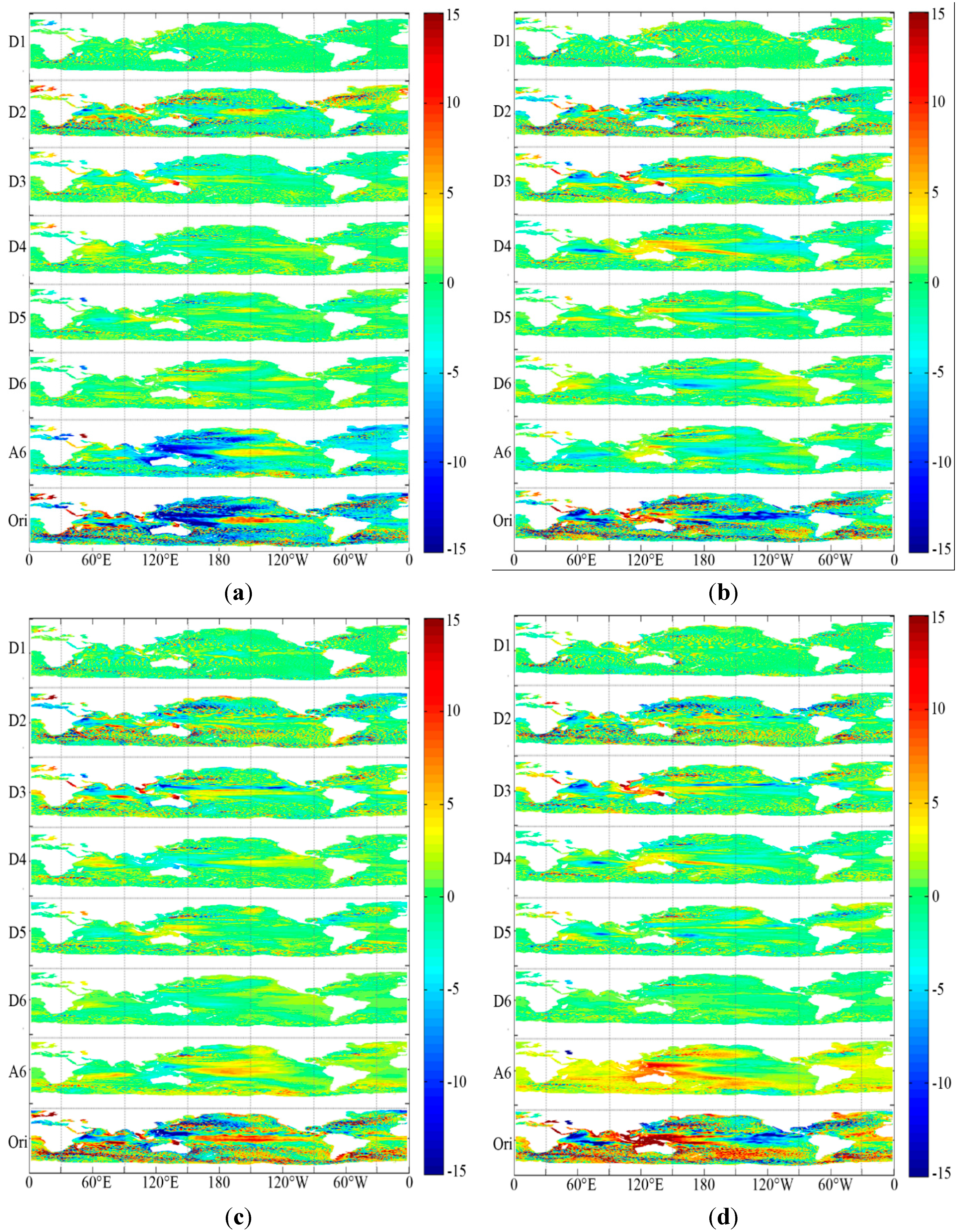
The reconstruction of the multi-scale components of the satellite altimeter data extracted from the multi-signal wavelet decomposition is depicted in
Figure 3. Since the full representation of all the data is impossible, we only provide several time slices. From the spatial dimension, the A6 components are much smoother than the original data. This suggests the multi-signal wavelet decomposition not only is multi-scale filter in the temporal domain, but also affects the spatial domain. Although the information of the generalized spatial scale affection of the multi-scale decomposition is still limited, in our cases, the larger temporal scales will also result in a smoother spatial distribution.
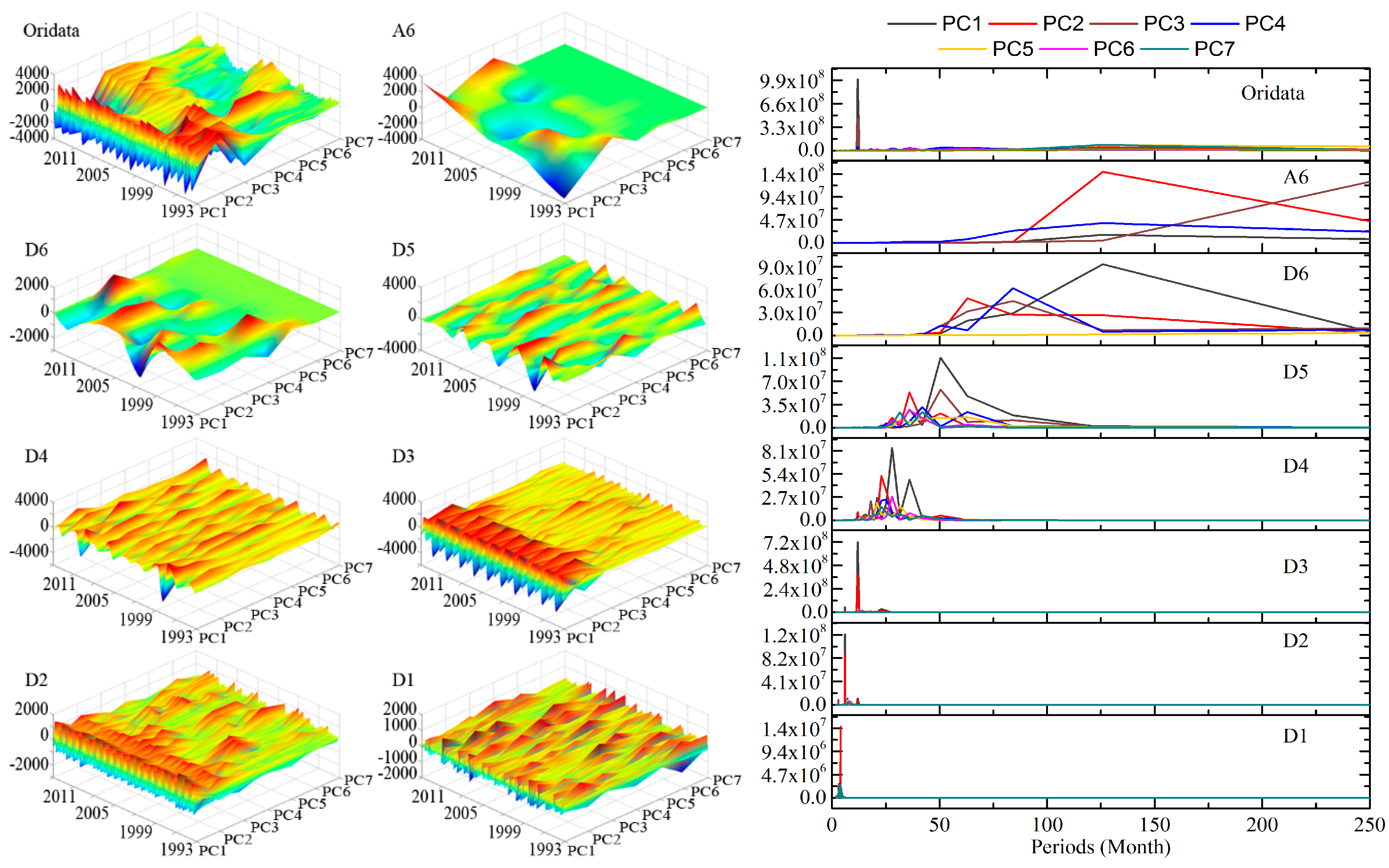
To reveal the detailed spatio-temporal distribution of the decomposed components at different scales, we applied the empirical orthogonal function analysis (EOF) to each decomposed component. The EOF method can extract the significant and common pattern of the spatio-temporal data. The variance contribution and the principal components (PCs), which suggest the consistency of the components across the spatial distribution and the significant temporal change of certain patterns, are extracted from the EOF (
Table 1). To further understand the temporal patterns of each decomposed component, the power spectrum (PSD) of each extracted PC is also calculated. The peak of the PSD suggests the significant period of the PC. The PCs and the PSD of the PCs are depicted in
Figure 4. To reveal the detailed frequency characteristics of the PCs, the highest peak of PSD and its associated frequency and period are extracted and represented in
Table 2.
Figure 3.
The multi-signal wavelet decomposition results. Four time slices are selected from the whole spatio-temporal data cubes of original data and reconstructed decomposed components ((a) January 1993; (b) January 1999; (c) January 2005; (d) January 2011). The color bar in each subgraph indicates anomaly range of the data. The multi-signal wavelet decomposition not only filters the data in the temporal domain, but also affects the spatial domain. Larger temporal scales will also result in a smoother spatial distribution.
Table 1.
Explanation of the Variance from the EOF of the Decomposed Result (%).
Table 1.
Explanation of the Variance from the EOF of the Decomposed Result (%).
| PC1 | PC2 | PC3 | PC4 | PC5 | PC6 | PC7 |
|---|
| Oridata | 31.2 | 27 | 16.2 | 10.5 | 5.5 | 4.9 | 4.3 |
| A6 | 63.7 | 16.2 | 10.7 | 9.1 | 0 | 0 | 0 |
| D6 | 31.7 | 23.7 | 22.9 | 19.8 | 1.7 | 0 | 0 |
| D5 | 31.5 | 15.4 | 13 | 11.5 | 10.5 | 9.3 | 8.4 |
| D4 | 31.2 | 17.8 | 11.8 | 11.2 | 10.4 | 8.8 | 8.4 |
| D3 | 52.4 | 27.8 | 5.2 | 4.2 | 3.5 | 3.4 | 3.2 |
| D2 | 32 | 22.8 | 9.8 | 9.6 | 8.8 | 8.5 | 8.3 |
| D1 | 16.4 | 15.6 | 14.7 | 13.6 | 13.3 | 13 | 13 |
Table 2.
Peak of PSD and corresponding frequency.
Table 2.
Peak of PSD and corresponding frequency.
| PC1 | PC2 | PC3 | PC4 | PC5 | PC6 | PC7 |
|---|
| Oridata | 0.0833 (12)/1.01 × 109* | 0.0079 (126)/4.45 × 107 | 0.0833 (12)/4.49 × 108 | 0.0833 (12)/5.33 × 107 | 0.0079 (126)/7.47 × 107 | 0.0278 (36)/2.62 × 107 | 0.0079 (126)/7.79 × 107 |
| A6 | 0.0079 (126)/1.67 × 107 | 0.0079 (126)/1.45 × 108 | 0.004 (252#)/1.27 × 108 | 0.0079 (126)/4.03 × 107 | 0.0119 (84)/1.73 × 105 | 0.0119 (84)/1.25 × 103 | 0.0159 (63)/2.26 × 102 |
| D6 | 0.0079 (126)/9.34 × 107 | 0.0159 (63)/4.84 × 107 | 0.0119 (84)/4.52 × 107 | 0.0119 (84)/6.18 × 107 | 0.004 (252#)/3.24 × 106 | 0.0198 (50)/1.65 × 104 | 0.004 (252#)/1.74 × 102 |
| D5 | 0.0198 (50)/1.06 × 108 | 0.0278 (36)/5.35 × 107 | 0.0198 (50)/5.73 × 107 | 0.0238 (42)/3.12 × 107 | 0.0159 (63)/1.59 × 107 | 0.0278 (36)/2.61 × 107 | 0.0238 (42)/2.35 × 107 |
| D4 | 0.0357 (28)/8.45 × 107 | 0.0437 (23)/5.17 × 107 | 0.0556 (18)/2.02 × 107 | 0.0397 (25)/2.42 × 107 | 0.0476 (21)/2.07 × 107 | 0.0357 (28)/2.71 × 107 | 0.0437 (23)/1.55 × 107 |
| D3 | 0.0833 (12)/7.18 × 108 | 0.0833 (12)/3.90 × 108 | 0.0714 (14)/1.85 × 107 | 0.0635 (16)/1.08 × 107 | 0.0595 (17)/1.22 × 107 | 0.0714 (14)/1.34 × 107 | 0.0754 (13)/1.52 × 107 |
| D2 | 0.1667 (6)/1.24 × 108 | 0.1667 (6)/8.81 × 107 | 0.1429 (7)/5.47 × 106 | 0.1389 (7)/1.12 × 107 | 0.1389 (7)/8.33 × 106 | 0.127 (8)/6.87 × 106 | 0.1349 (7)/4.71 × 106 |
| D1 | 0.25 (4)/3.11 × 106 | 0.25 (4)/1.44 × 107 | 0.254 (4)/2.87 × 106 | 0.2619 (4)/2.89 × 106 | 0.2579 (4)/2.26 × 106 | 0.3135 (3)/1.41 × 106 | 0.2659 (4)/2.75 × 106 |
From
Figure 4, we can find that the PCs of the original data, which are not easy to separate, are very similar. The PSD suggests that most of the PCs of original data have strong annual cycle. Most of the differences between different PCs are the phase difference caused by the spatial distribution lag. However, the PCs and the PSD of the PCs suggest the decomposed components are much more separable. The dominant periods of the PSD of each component are significantly different. The major period of the components from A6 to D6 is changing from inter-decades to bi-month. In addition, the PSD of each EOF at each scale can also be classified. This indicates that the patterns of the spatial different are also clearly extracted. The multi-scale decomposition can clearly improve the pattern classification of the data.
Figure 4.
The principal components of original data and each decomposed components and their power spectrums. The 3D plot of the principal components of original data and each decomposed components (left); and the power spectrums of each decompose data of each principal component of original data and each decomposed component (right). The frequency is changed into period for better illustration.
From the explanation of the variance from the EOF of the decomposed result, the A6 and D6 components are much simpler than the other components, which have fewer principal components. This suggests large-scale variations are more consistent and smooth. Although, the PSD for the time series that are longer than half periods of the whole data length are not very accurate, the combining investigation from the PCs also suggest that both A6 and D6 are inter-decade variations. The A6 components have a period of ten years, which can be seen as the long-term trend of the data. Meanwhile, the D6 components have a quasi-period of 5–7 years. The strong spatial variation in the Equatorial Pacific and Indian Ocean suggests D6 may have close relations to the significant ENSO variations. The D5 and D4 components are also inter-decade variations, which have spatial distribution around the global oceans. The spatial distribution also suggests these two components may also have close relations with the ENSO events. D3 component, which has very high variance contribution of the first PC, has a significant annual cycle. Since the yearly period is the most common and significant period all around the global ocean, the significance of the yearly cycle also proves the consistency of the EOF. The D2 and D1 components have periods of half-a-year and two to four months, respectively. Some irregular high frequency noise is also contained in these components.
From the above discussion, the multi-signal wavelet decomposition can well extract the multi-scale temporal variation from the original multi-temporal remote sensing data. The decomposition is performed in the time domain but also affects the spatial distribution. The decomposed components have clear temporal variation with significant temporal period. By the multi-scale decomposition, the features of original data are much more separable. Thus, it will be very useful and helpful for feature extraction and data segmentation at different scale levels.
4.3. Feature Clustering Result
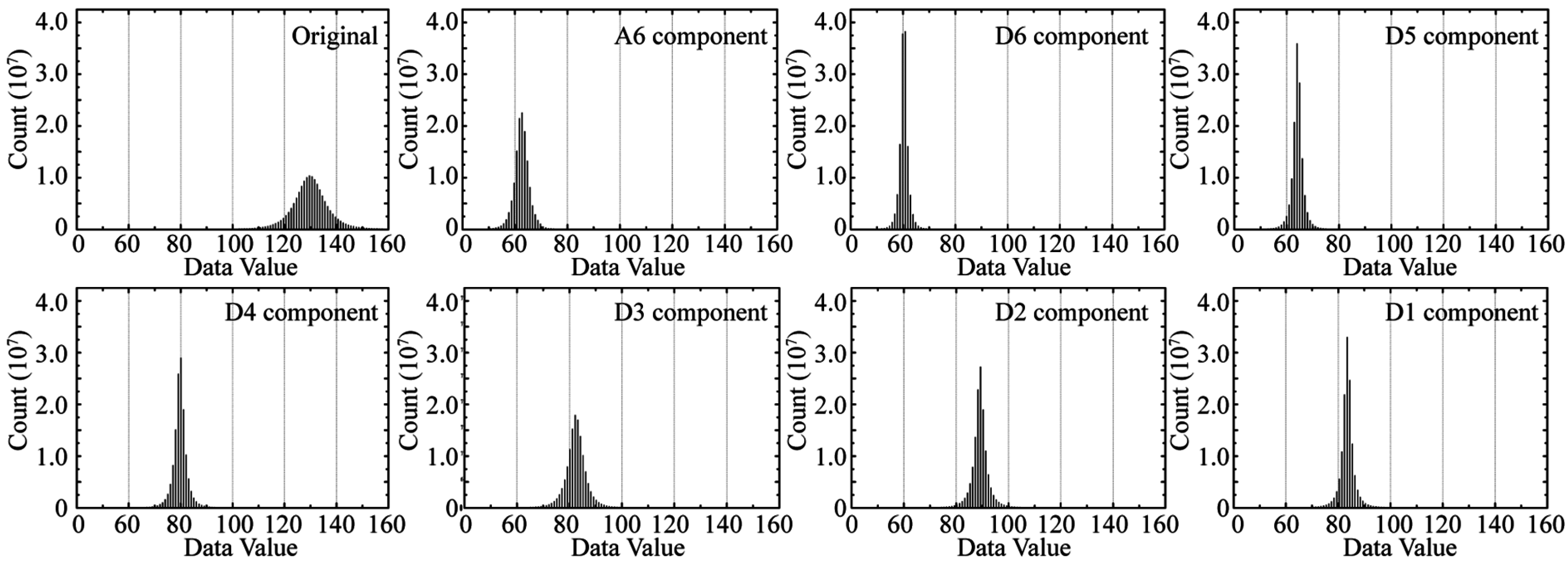
The integer approximation and the histogram representation of each decomposed component are performed for the feature clustering. The histogram of the original data and the decomposed multi-scale components are shown in
Figure 5. The original histogram only has a wide band peak, because various spatial features are blended together. For this case, it is not very easy to classify different patterns directly from the original histogram. The histogram of the decomposed components is much more separable. Each histogram of the decomposed component has narrow bands and clear single peaks. The values of A6, D6 and D5 are smaller than those of D4–D1 component. This corresponds to the situation where the variation amplitude of the inter-decade cycles is lower than that of the inner-decade cycles in most areas. The segmentation based on the histograms of all the decomposed components is much more structurally clear than segmentation based on the histogram of original data. The cluster distribution of the histogram bins also suggests that the data are more significant and separable than the original data.
Figure 5.
The histogram of the original data and the decomposed components.
Figure 5.
The histogram of the original data and the decomposed components.
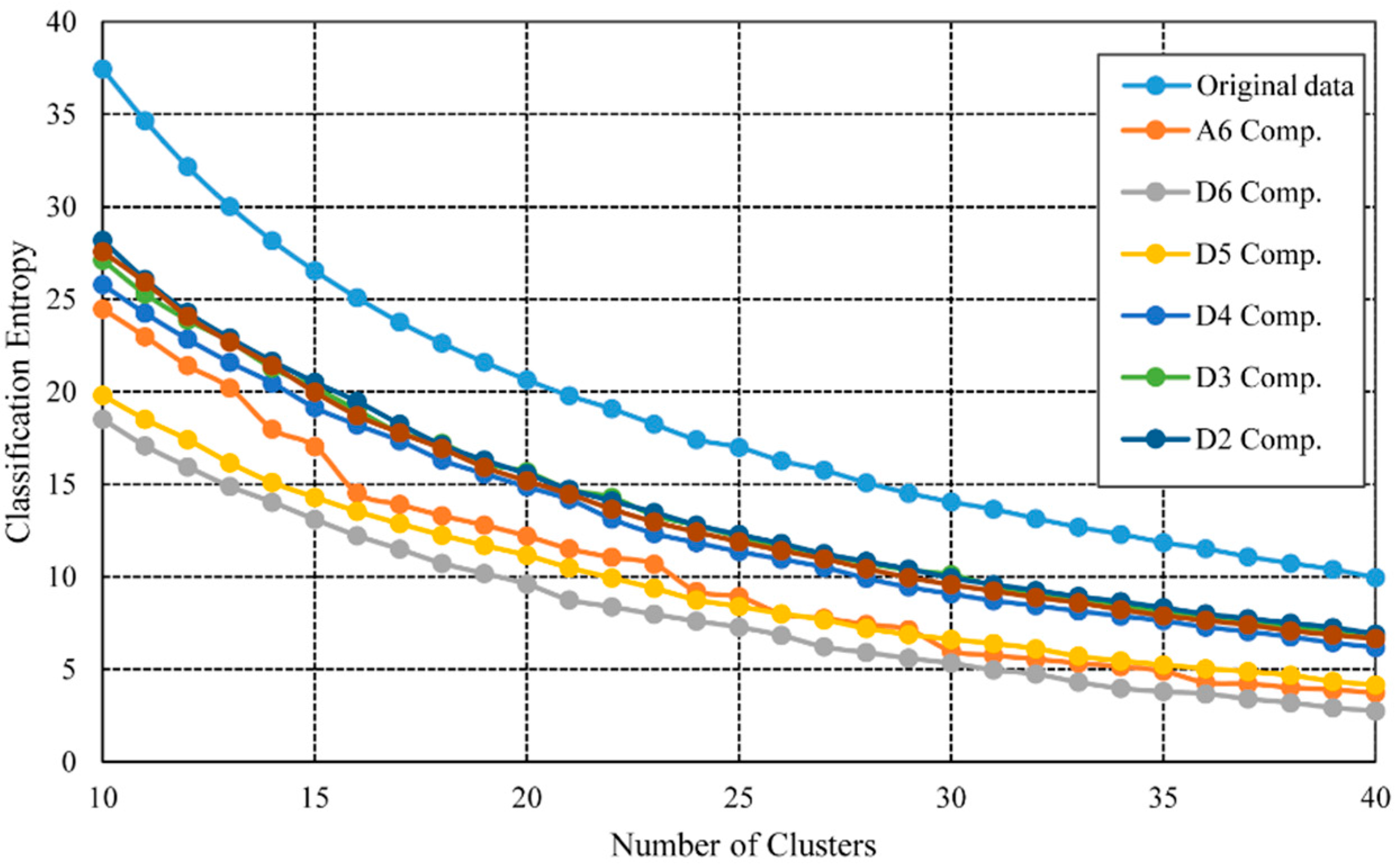
Before the final feature clustering at each decomposed component, the optimized cluster number of each decomposed component is calculated from the simulation of the CE index changing according to the cluster number. The simulations are constructed by changing the number of the Clusters from 10 to 40. For each cluster number, the CE is calculated and logged.
Figure 6 suggests how the CE changes according to the cluster number at each scale. For all decomposed components, the value of CE grows lower when the cluster number increases. The CE of the original data is significantly higher than that of the decomposed components. And the D1–D4 components have very similar CE. The CE of D5 and D6 components is also very similar, and they all have very low CE values. Unlike other components, the CE of A6 does not change smoothly, which suggests that the complexity degrees of the A6 component may be different. These suggest that the complexity of the inter-decade variations is lower than that of the inner-decade variations. This is partially because the inter-decade variations are much smoother and change more slowly and partially because fewer noises are contained in the long-term variations. We will notice that in the lower sections the D5 and D6 are mainly influenced by the ENSO event, which is an irregular phenomenon in both spatial and temporal dimensions. Thus this kind of irregularity in CE also demonstrates the characteristics of the signal.
Most of the CE at different scales is changing very slowly after the cluster number gets bigger than 30. This suggests that the clustering with the cluster number bigger than 30 will not produce lots of different information. Therefore, we can consider that the minimal number of 30 will well represent the distribution and feature of original data. Thus, we select the optimized cluster number of 30 for all the decomposed components to produce the final segmentation. Although, it is optimal to select the different optimal cluster number for each level, we select the optimized cluster number of 30 for all the decomposed components according to CE for simplicity.
Figure 6.
Determination of Cluster Numbers.
Figure 6.
Determination of Cluster Numbers.
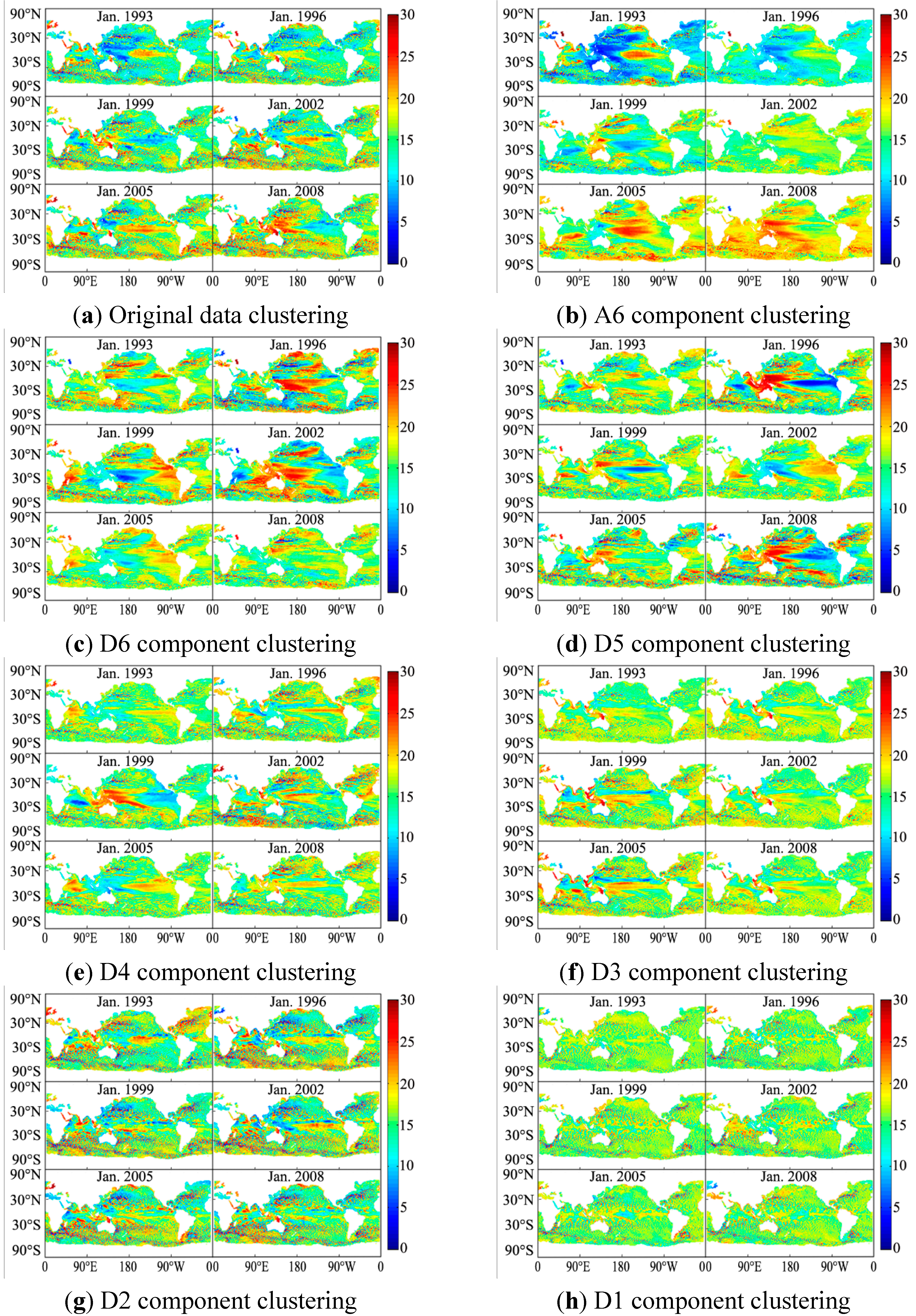
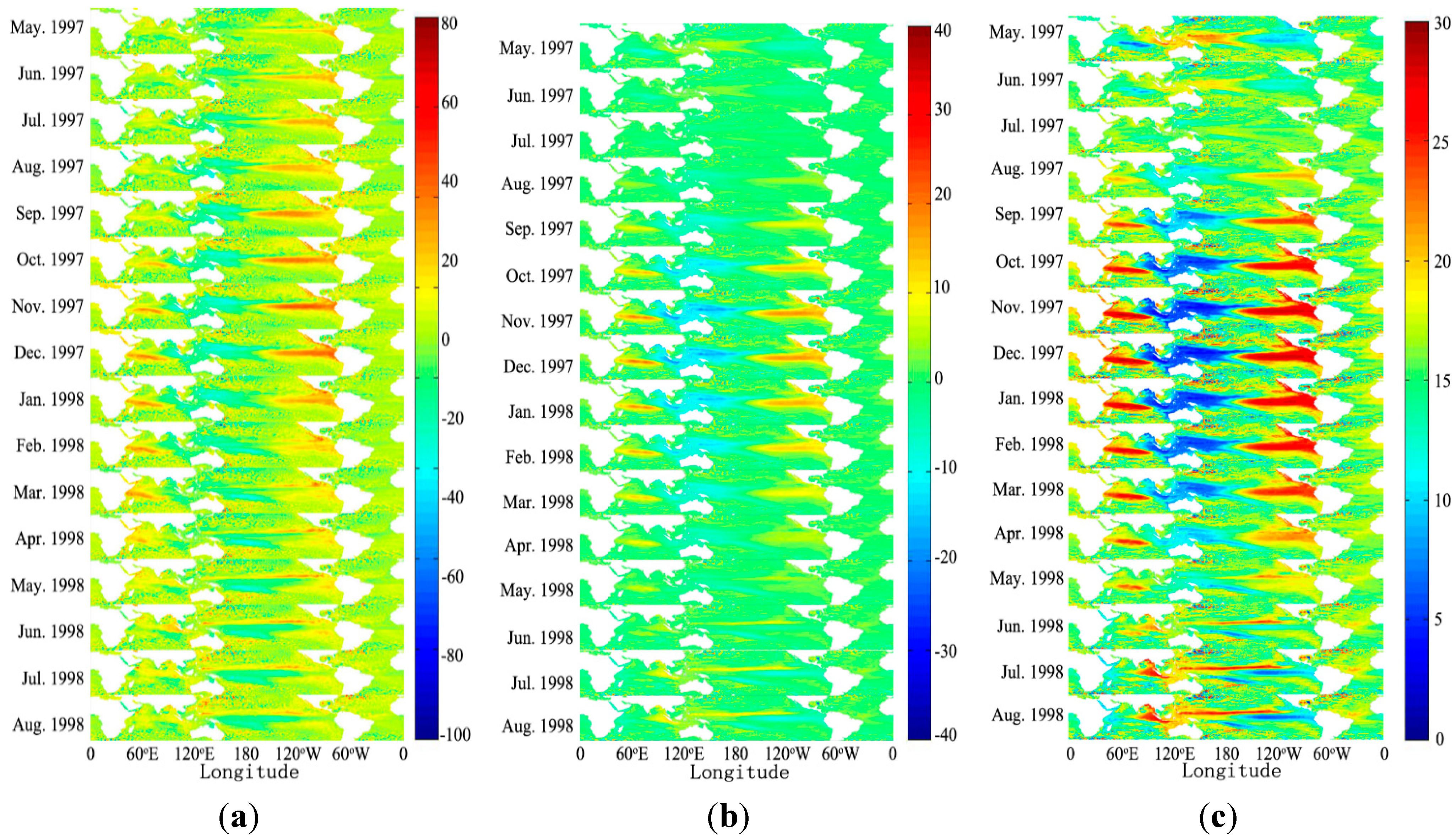
The feature clustering with the cluster number 30 is performed to each histogram of the decomposed components. The spatio-temporal distribution of the segmented result is shown in
Figure 7. The cluster of the original data does not have a clear significant spatial structure. Lots of small patches can be found in the cluster result, which suggests the original segmentation cannot well separate the variations at different temporal and spatial scales. The cluster result of the decomposed components has much clearer spatial structures. The cluster result of the A6 component suggests clearly two stages before and after the year 2003. This is consistent with the trend change of the sea level height. The cluster result of the D6–D4 components is much more significant in the time dimension. The major changes are the spatial pattern changes crossing the global. Since these components mainly reveal the ENSO signal, detailed comparison of the spatio-temporal changes during ENSO events can be achieved. From the temporal cluster index changes, the evolution process, including the starting, growing, peaking, weakening and vanishing, is much clearer than the original data. The clustering of the D3–D1 components mainly changes periodically through the time which suggests that our cluster can well represent both the spatial and temporal changes of the data. All the above suggest our approach can be used as an exploring tool to find patterns in the spatio-temporal data. Unlike tensor methods, our approach can support irregular data that contain missing data at any spatial locations.
Figure 7.
The cluster results of the original data and the decomposed components: (a) cluster result of the original data; and (b–h) cluster results of A6, D6, D5, D4, D3, D2, and D1 components, respectively. The color bar in each subgraph indicates the classification type index of the data. Due to the space limits, only six time slices are selected for demonstration.
6. Discussion
In our approach, the multi-signal wavelet decomposition was only used to decompose the multi-temporal remote sensing data along the time dimension to extract the temporal multi-scale variations. However, the channel-to-channel (location to location) relations at different scales during the decomposition, which also reveal the spatial interaction and distribution of the signal at certain temporal scales, are not fully studied. Revealing the detailed channel-to-channel relations during the decomposition and further integrate them in spatio-temporal feature cluster may also very helpful. In the integer representation, the adaptive selection of the bins to construct the histogram is important for data that have closed value in a very narrow band of the integer. Selecting the threshold adaptively according to the data value distribution to construct the histogram can solve this. The information or morphology criteria (e.g., entropy) can be used for the adaptive histogram construction. However, special attention should be paid to avoid the pseudo mode that may be produced by the equalizer. Since both the integer representation and the histogram representation are very fundamental representations, more advanced approximation in the time-frequency space (e.g., the representation of the data with Fourier basis or wavelet basis) may produce much better results. With the spectrum representation theory, the characteristics of the data may be extracted with much more details at a much lower computational cost.
The histogram re-organize similar data values into a single histogram bin, it interlinks the value distribution and the spatio-temporal distribution of the data. The integer representation, which is simple and efficient, not only enhances the feature pattern but also reduces the computational complexity. The soft threshold of the FCM results applied to the histogram can results in more consistency and continuity of the spatio-temporal feature cluster. In addition, the cluster is data adaptive, and a prior knowledge about numbers of objects/features and the distribution of the original data is not required. However, the cluster performance of the method can still be improved in several aspects. In the FCM, the selection of the optimal cluster numbers is still experimental and the efficiency of the selection procedure can also be optimized. In the reversed mapping procedure from the cluster of the histogram to the original data type, the constraints of spatial continuity can be integrated, which can further control the fine level of details of the cluster.


