Walk This Way: Improving Pedestrian Agent-Based Models through Scene Activity Analysis

Abstract

Pedestrian movement is woven into the fabric of urban regions. With more people living in cities than ever before, there is an increased need to understand and model how pedestrians utilize and move through space for a variety of applications, ranging from urban planning and architecture to security. Pedestrian modeling has been traditionally faced with the challenge of collecting data to calibrate and validate such models of pedestrian movement. With the increased availability of mobility datasets from video surveillance and enhanced geolocation capabilities in consumer mobile devices we are now presented with the opportunity to change the way we build pedestrian models. Within this paper we explore the potential that such information offers for the improvement of agent-based pedestrian models. We introduce a Scene- and Activity-Aware Agent-Based Model (SA²-ABM), a method for harvesting scene activity information in the form of spatiotemporal trajectories, and incorporate this information into our models. In order to assess and evaluate the improvement offered by such information, we carry out a range of experiments using real-world datasets. We demonstrate that the use of real scene information allows us to better inform our model and enhance its predictive capabilities.

1. Introduction

Pedestrian movement is woven into the fabric of urban regions. From private indoor to public outdoor spaces, pedestrians are constantly utilizing their surroundings to reach destinations, exploring their environment, and to achieve specific goals. Yet, in spite of the ubiquity of pedestrian movement, understanding how pedestrians move in and explore the space around them remains a fundamental scientific challenge. This challenge has significant practical implications, ranging from improving the design and functionality of urban spaces to emergency response and disaster recovery. Intensifying urbanization trends are leading to a growing urban population, which according to some predictions will reach 6.3 billion by 2050 [1], or approximately two thirds of the world population at that time. This trend emphasizes the need to gain better insights into how pedestrians move in and utilize urban spaces.

Pedestrian models describe the patterns of movement of individuals or groups in a scene over space and time, whereby a person’s current position is based on its old position, desired destination, and surroundings, including the physical environment and other people [2]. Such models are widely used to simulate activities of crowds for planning and evaluation from an individual’s perspective (see [3] for a review). By modeling the individual and exploring how individuals interact over space and time, researchers can observe the emergence of crowds from the bottom up. One technique that is inherently suited to modeling individuals, or groups of individuals, is that of agent-based modeling. Agent-based models (ABMs) have been used to explore a wide range a phenomena from the individual perspective, ranging from: animal movement [4]; agricultural practices [5]; land use change [6]; residential segregation [7]; crime [8]; to daily travel patterns [9]. With respect to pedestrian movement, ABMs have been used to explore a number of problems such as navigation in confined spaces, such as art galleries (e.g., [10]); navigation through town centers (e.g., [11]) and shopping malls (e.g., [12]); public gatherings and festivals (e.g., [13]); riots (e.g., [14]) and egress from a building (e.g., [15]).

Simulations with agent-based models serve as artificial laboratories where we can test ideas and hypotheses about phenomena which are not easy to explore in the real-world, especially for phenomena where understanding both the relevant processes and their consequences are important [16]. For example, such simulations may offer us insights on the manner in which people evacuate a building during a fire. We can model a building in an artificial world, based on geographical accurate building floor plans, and populate it with agents representing artificial people. These agents are given a set of behaviors that are often based on empirical or qualitative data. Then, the researcher can initiate simulated events (e.g., a simulated fire), and observe how these agents react, including the cascading ramifications of their reactions (e.g., bottlenecks, stampedes [17]). This allows us to test numerous scenarios in order to gauge the effects of a real-life events and improve our planning capabilities, assessing for example, how various building layouts and room configurations can impact evacuation time [18].

The quality of these simulations depends heavily on the model used, as well as the physical (e.g., walking speed) and behavioral attributes (e.g., distribution of traffic volume within a scene and the agents’ cognitive models) that are used to describe pedestrian movement. In essence, such attributes convey our understanding of peoples’ movement in space, and to accurately assign these attributes data is needed. However, the pedestrian modeling community has been and still is relying primarily on ad-hoc and limited-scale data for validating these models [3,19]. There has also been some limited work on tying these models to microscopic pedestrian characteristics as they may be extracted by other sources (e.g., [20]). However, this was in the context of approaches like the social forces of Helbing and Molnar [21], which assume all pedestrians respond to “forces” around them and have no internal cognition guiding their behaviors [22]. This is clearly not the case of real human beings which have intrinsic properties [3]. That being said, the complex nature of human behavior renders all models mere abstractions of reality, posing challenges to both force and rule-based models. Moreover, as Torrens et al. [23] also note, collecting data pertaining to individual walking paths is a challenge and is an active field of research [20,24], which still needs to be addressed if we are going to make high fidelity pedestrian models.

Recent technological advances offer an opportunity to change the way we construct and calibrate pedestrian models. In particular, the proliferation of video surveillance and enhanced geolocation capabilities in consumer mobile devices (e.g., embedded global positioning system (GPS), Wi-Fi, or radio-frequency identification (RFID) capabilities in smart phones or tablets), particularly in urban regions, now enables us to generate unprecedented amounts of pedestrian mobility datasets [23,25], which offer a wealth of information at a fine spatial and temporal resolution. All these sources can generate massive amounts of spatiotemporal mobility datasets, as part of the emerging era of big spatial data [26]. Tapping into this information to improve pedestrian modeling remains a rather underexplored area, and this is the topic addressed here.

In this paper we present an approach to enhance simple path-based pedestrian models through the use of real trajectory data in order to improve their accuracy for simulating and predicting pedestrian movement. More specifically, we use actual pedestrian tracks and the meta-information derived from them to calibrate a simple ABM, and we show how this improves performance, allowing the ABM to better match the behavioral characteristics of the actual scene. Thus, by combining a simple model with real scene data we produce a powerful tool to generate reliable simulations of pedestrian movement patterns. The value of incorporating this information is twofold. First, the use of real data (e.g., derived from tracking) to describe behavioral attributes of the agents rather than relying on generic parameters advances our capabilities to model human movement in ABMs (e.g., their velocity, and the rate at which they enter/exit a scene). Second, trajectory patterns reveal the underlying structure of each scene as it is defined through human activities. As such they communicate peoples’ perceptions of the space allowing us to move from a pure geometric approach (e.g., using floor plans) that considers only form, to one that takes into account how people use the space i.e., its function as well [27]. Using such information to inform an ABM allows us to tailor its application to the particularities of various scenes. We refer to this approach as a Scene- and Activity-Aware ABM (SA²-ABM).

For example, utilizing tracking data to extract entrance and exit locations of pedestrians offers to the ability to consider both physical entrance and exit points (e.g., doors) and behavioral entrance and exit points (e.g., a region in an open space used by most pedestrians to enter an atrium), while tracking pedestrians’ movement between entrances and exits allows us to estimate locomotion parameters and mobility patterns within that space. By combining these two components (pedestrian locomotion, navigation and behavioral parameters, and physical space) into a single pedestrian model, it is possible to explore and predict the behavior (i.e., routes) of pedestrians. In this paper we will present an approach to collect and analyze tracking data in order to inform an ABM. Using as a test case an indoor scene. The remainder of the paper is organized as follows. In Section 2 we present an overview of our modeling framework. In Section 3 we describe our activity-driven scene models, before moving onto the ABM (Section 4). We then move on to show a number of experiments using the data from the activity scene models and the ABM (Section 5) and in Section 6 we provide a summary of the paper and an outlook for further work.

2. Approach Overview

The motivation for our approach stems from the rapid growth in the availability of mobility information in the form of spatiotemporal trajectories [28]. Mobility data can be collected through various geolocation capabilities, e.g., through the use of cell-phones (e.g., [29,30]), RFIDs (e.g., [31]) and GPS (e.g., [32,33]). These well-established approaches for mobility data collection are further complemented by emerging alternative techniques such as the use of data derived from WiFi technology [34] and even general communications data at large [35].

From among these various techniques that are available for the generation of mobility information we choose as reference for our work that of video surveillance, as it is capable of generating large numbers of trajectories for a given scene, thus providing us with a greater understanding of the common activity patterns over that area, as compared to the sparse samples over broader areas that are provided by alternate mobility capture techniques. Furthermore, video surveillance is also becoming widespread. Video surveillance systems are deployed indoor and outdoor to a wide variety of facilities, ranging from hospitals, schools, and shopping malls to airports, government facilities, and military installations. As an indicative reference, it is estimated that in the city of Chicago there are approximately 10,000 video cameras deployed for this purpose [36]. In the UK, as of a few years ago, it was estimated that between 2 and 4 million closed-circuit TVs (CCTVs) were deployed, with over 500,000 of them operating in London alone [37,38].

In order to take advantage of this data for ABMs we propose an approach that makes use of information extracted from such trajectory datasets to improve the accuracy of modeling. In the context of this paper we use the term “accuracy” to refer to the degree to which the results of the simulation resemble the real data in the scene. We should mention here that even though we are focusing on pedestrian movement, a similar approach could also be applied to other types of movement (e.g., car traffic). As we see in Figure 1, we proceed by analyzing real trajectory data to derive activity knowledge in the form of heat maps representing aggregations of trajectories over a period of time, and statistics on frequency of entrance/exit usage within our scene. Within this paper we use the term heat map to refer to representations of aggregate activity (general trends) within the scene, which could be considered as a “occupancy” or “density” map (as discussed in [39,40]). We then use this information to improve a basic ABM by informing its parameters with locomotion (e.g., walking speed) and behavioral attributes (e.g., distribution of traffic volume within a scene) for the scene, thus generating a Scene- and Activity-Aware ABM (SA²-ABM) as we will be discussing in Section 4. We will demonstrate through the experiments in Section 5 that this allows us to improve the accuracy of our simulations, thus enhancing their suitability for forecasting.

Figure 1. Approach flowchart.

Figure 1. Approach flowchart.

Figure 1 shows an overview of the processing steps in our approach. In the first step, we assume pedestrian movement data is collected through a video surveillance system, resulting in a set of trajectories. It should be noted that although we use a video system in this overview, other geolocation technologies (e.g., GPS) could also be used, assuming that they provide us with sufficiently dense and representative datasets for the area of interest. In the second step, we model the observed scene based on the pedestrian activities derived from the trajectories. This includes the detection of entry and exit points, movement patterns between such points, and the locomotion parameters for each pattern. As a result of this step, a detailed model of the scene (including its structure, the pedestrian locomotion and behavior parameters, and movement patterns) is derived. In doing so, we capture not only explicit information (e.g., entrance and exit points), but also implicit (e.g., popular paths, obstacles) that is often missing from floor plans, layouts or other means that are commonly used up to now to construct the space in which the simulation takes place. This model is then used to construct a SA²-ABM, which can be compared to the observed scene data and refined accordingly. Once constructed, the SA²-ABM can be used to provide forecasts through simulations under varying conditions (e.g., exploring how an on-going event can develop under various conditions). This process can be implemented periodically, introducing various parameters one at a time, in order to identify the contribution of each one, thus avoiding unnecessary computational overloads.

3. Harvesting Scene Activity Information

The analysis of spatiotemporal trajectories has received wide attention within the geospatial and database communities over the last decade, starting with the introduction of a variety of approaches to index them for post-processing (e.g., [41]). From among the large body of work that has led to the current state-of-art on computational movement analysis [28] we can identify as relevant to our work the development of complex object tracking approaches through cluster-based [42], non-cluster-based [43] and data mining-derived pattern movement-based approaches like the TMP-Mine approach of Tseng and Lin [44]. Advancing the analysis level to extract semantic information for the captured trajectories we had the work of Spaccapietra et al. [45] towards a semantics-driven approach to trajectory analysis, considering stops and moves to understand actions and activities. Bogorny et al. [46] built on this foundation, presenting a framework for semantic pattern mining and its implementation in Weka-STMP. Despite these advances, the efforts to identify scenes characterized by distinct patterns of activity are rather limited within the GIScience and database communities, with a notable exception being the TraClass framework of Lee et al. [47] who presented an approach that was hierarchical, region-based (identifying regions where specific types of trajectories have a dominant presence), and trajectory-based (analyzing trajectory partitions).

In parallel to these efforts of the geospatial and database communities, the computer vision community has been addressing the modeling of scene activities in the context of surveillance applications at various levels of detail. Within this context, a group of approaches has focused on detecting scene layout in structured environments (e.g., building entrances/exits, sidewalks, roads, intersections) to support surveillance applications through activity annotation. Makris and Ellis [48] have presented an approach for learning scene semantics (e.g., entry and exit zones, junctions, paths) from a stream of video using unsupervised methods. More recently, Nedrich and Davis [49] identified coherent motion regions from tracking data and applied this information to detect scene structure. Kembhavi et al. [50] developed a video understanding system to identify various scene elements, such as roads, sidewalks and bus stops, using probabilistic models within a Markov logic network framework. From a perspective of categorical object recognition to scene analysis, Turek et al. [51] proposed an approach to analyze a video scene based on the behaviors of moving objects in and around them.

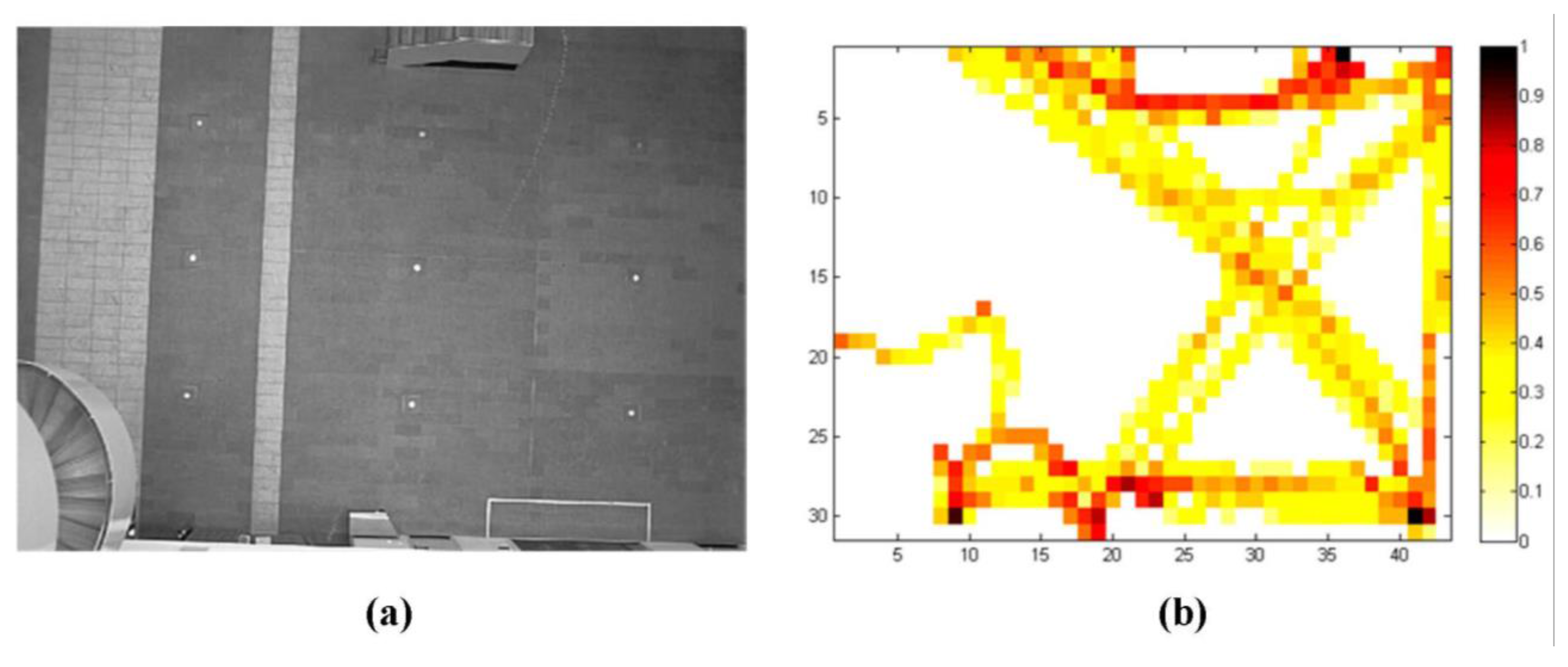
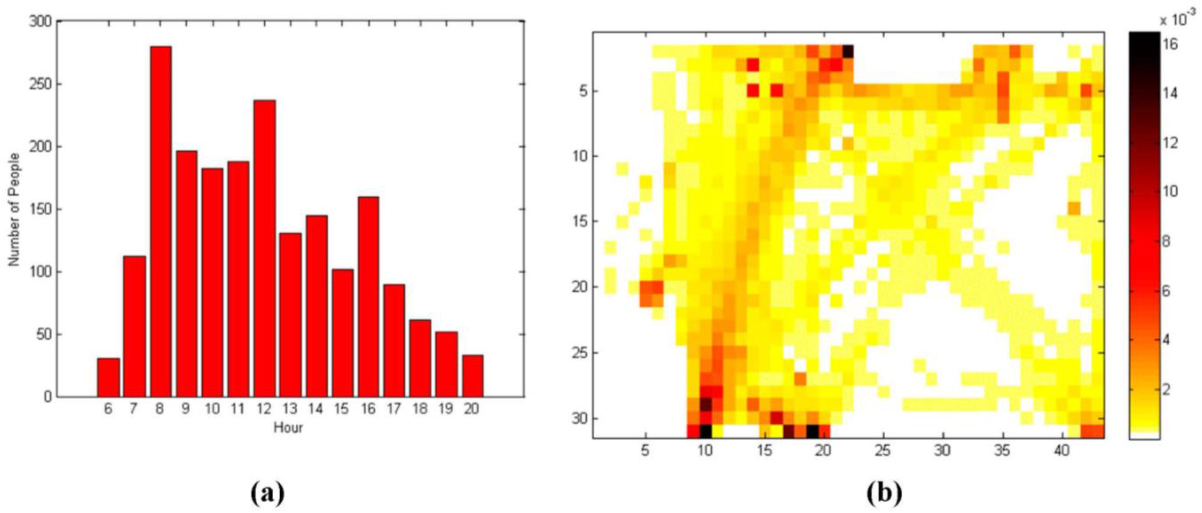
Figure 2. (a) A scene; and (b) its corresponding activity heat map that shows an aggregation of trajectories in that scene over a period of one hour. White tiles mark areas that remain unvisited during that period, and as the values grow the coloring scheme proceeds from white to yellow, and red for the most visited tiles in the scene.

Figure 2. (a) A scene; and (b) its corresponding activity heat map that shows an aggregation of trajectories in that scene over a period of one hour. White tiles mark areas that remain unvisited during that period, and as the values grow the coloring scheme proceeds from white to yellow, and red for the most visited tiles in the scene.

Another group of approaches has focused on segmenting dominant motion patterns (e.g., vehicles turning, pedestrian crossings) for scene understanding. For instance, Wang et al. [52] proposed a hierarchical Bayesian model to find typical “atomic” activities and interactions in complicated scenes (e.g., vehicles stopping for pedestrians to cross the street). Singh et al. [53] focused on unusual activity detection, for example people carrying or abandoning objects. Xu et al. [54] provided a spatiotemporal analysis of campus scenes monitored by an outdoor camera network. They applied the average optical flow within a short duration to represent the crowdedness of the scene, and explored the relationship between activity patterns and campus class schedule. Girgensohn et al. [55], worked on comparing activities through the use of heat maps.

As the aggregate tracking information we have is in the form of a heat map [56], and since the objective of the ABM in the context of this publication is also to generate patterns of movement at the aggregate level, we chose to proceed by using activity heat maps as aggregate spatiotemporal expressions of trajectories crossing a scene of interest. This facilitates a direct comparison between the pedestrian model and the scene data. An activity heat map expresses how frequently a specific location in a scene is visited by a trajectory. For example, let us assume that we have as input for our analysis a set of m trajectories captured in a scene:

TRJ = {trj₁, trj₂, trj₃, …, trj_m}

(1)

Each trajectory trj_i comprises a sequence of trajectory points, in the form of a set of time-ordered coordinate pairs (x_i(t), y_i(t)):

trj_i = { (x_i(t_start),y_i(t_start)), …, (x_i(t_end),y_i(t_end)) }

(2)

where each coordinate pair indicates the recorded location of a tracked individual i at time t. Then, the activity heat map for this scene is estimated by tessellating the space into square cells and assigning to each cell a heat value h that is a function of the number of crossings of this cell by our set of trajectories. More specifically, the heat value h(x,y) of a cell with coordinates (x,y) in our scene space is the normalized metric:

$$h(x,y)=\frac{cross(x,y)-\min (cross(\cdot ,\cdot ))}{\max (cross(\cdot ,\cdot ))-\min (cross(\cdot ,\cdot ))}$$

(3)

where cross(x,y) is the number of trajectories that cross cell (x,y), min(cross(⋅,⋅)) (and max(cross(⋅,⋅))) are the minimum (and maximum respectably) among the set of all crossing values cross(⋅,⋅) in our scene. In this equation (⋅,⋅) refers to two cells between which a crossing occurs. Figure 2 shows the physical scene (left) and its corresponding activity heat map (right). Heat maps are often used for analyzing indoor and outdoor space activity (e.g., [55,57]). For our methodology, heat maps offer two distinct advantages. First, it naturally conveys knowledge about the scene: as an example, it allows us to identify popular paths (connecting the lower right to the top left in Figure 2). Second, it allows us to visualize connections in space: each cell has 8 neighbors (e.g., the Moore neighborhood), and by comparing the corresponding heat values, we can calculate an informed estimate on the most likely next step given a location along a trajectory, which is particularly suitable for the simulation problem that we are addressing (see Section 4.4.2). We complement this heat map with entrance and exit locations for our scene (identified trivially as clusters of locations where trajectories start and end respectively) and a frequency table showing entrance-exit connections (also identified trivially from the trajectories) to provide a comprehensive yet easy to use activity-based model of our scene that will drive the application of our SA²-ABM.

4. The Scene- and Activity-Aware Agent-based Model (SA²-ABM)

The purpose of SA²-ABM is to enhance a basic ABM through a simple set of rules identified using the activity-driven models of Section 3. This ABM is enhanced by simple behavioral rules that are presented below in order to produce more realistic patterns of pedestrian movement. These rules are informed by real pedestrian movement data and information about the physical environment through which the pedestrians are moving, as discussed in Section 3. We supplement this with other data from the literature of pedestrian movement where necessary. For example, it is well known that people walk at different speeds (e.g., [58,59]); from analyzing our particular scene information we found the maximum walking speed to be 1.5 m per second and this is what we use in the model for the maximum walking speed of our agents. Nelson and Mowrer [60] also note that humans have a psychological preference to avoid bodily contact, defined by Fruin [59] as the “body ellipse”. Within this model, we set for computational simplicity the agent size to be 37.5 cm by 37.5 cm (accounting for their anthropomorphic dimensions and body ellipse [61]), as we are using an enclosure representation of a regular lattice which often treats all agents as having the same size. Alternate approaches employing continuous space representation would allow for varying sizes of pedestrian agents (e.g., to match the corresponding sizes extracted from the video feeds [62]), but at substantial computational costs [63]. Such detailed representations of the size of the pedestrians without the transition to a continuous space would not impact the results considerably of the following ABM (this might be different if we were looking at bottlenecks or evacuation from confined spaces).

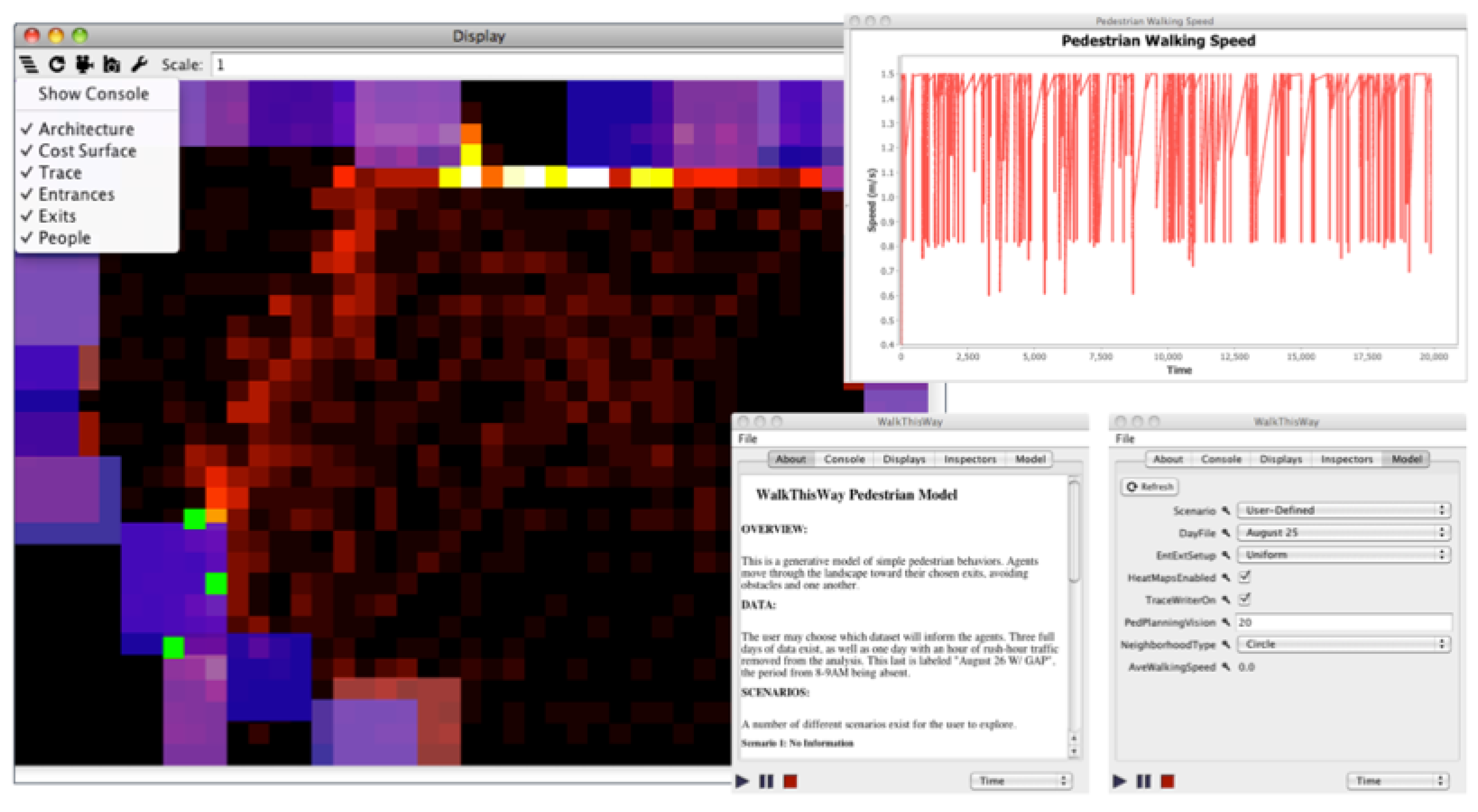
The SA²-ABM is programmed in Java using and extending the MASON Simulation toolkit [64]. We have provided an executable of the model, source code, and all data presented in this paper at https://www.openabm.org/model/4706/version/1 to aid replication and experimentation. In Figure 3 we show the graphical user interface (GUI) of the model. Clockwise from the top left, the GUI features a map with the option to view or hide any layer of data, a graph that summarizes walking speeds over time, and the model controller. The model controller allows the user to initialize, pause, or stop the simulation, control which displays are hidden or shown, and view some basic model information along with running the different scenarios presented below. Such an interface allows for ease of use in understanding and debugging the model [65].

Rather than taking a forced-based modeling approach (e.g., [21]), which often treats people as responding to “forces” exerted by others and the environment which some would argue creates an ecological fallacy in assuming pedestrians have no internal decisions making capabilities [3,63], here we focus on the actions of individual entities (i.e., a rule-based approach, see [22] for a discussion of the differences) in a cell-based environment (similar to the work of [13]). Route-choice is a critical component of any pedestrian model, as it describes the dynamic process through which people move through a scene, making and reassessing decisions as time progresses and scene traffic changes with it. Route choice is an active area of research which spans multiple disciplines such as psychology [66,67], geography [3], engineering [68,69], computer graphics [70,71], to name but a few. Computationally, this is a challenging issue, both in terms of theoretical and practical problems associated with describing pedestrian behavior. Two common approaches for route-choice are shortest path and following signage [69]. The shortest path approach is based on the notion that individuals wish to minimize the distance they have to walk, and this is not necessarily the route indicated by signage. However, it needs to be noted that the shortest path might not be the quickest path, for example if there are many pedestrians along the shortest path, this will slow down the agents. To calculate the quickest path one needs consider dynamic routing [68]. Both the shortest path and following signage approaches relate to the pedestrians enclosure perspective, which varies when they know or do not know their environment. People familiar with the building would have intrinsic broader knowledge of it (i.e., they are able to calculate the shortest path), whereas visitors with limited knowledge of building layout are more likely to follow emergency signage [68,72]. Here we choose the simplest option where pedestrians initially follow the shortest path between entrance and exit but as they have a line of sight and carry out dynamic route-planning to avoid obstacles and other agents (see Section 4.4.2) they in essence find the quickest route. This is also consistent with the size of the area under consideration, where intrinsic knowledge of the environment does not greatly affect routing decisions, which are driven instead by the visual identification of entrances and exits. Work by Hillier et al. [73] reinforces this idea, in the sense that they demonstrated that the majority of human movement occurs along lines of sight Also, as is common in many ABMs of pedestrian movement, we have preplanned entrance and exit locations (see Section 4.4.1) based on information from the scene itself (as discussed in Section 3) but the choice of route is determined at run time. The remainder of this section describes in detail the ABM following the overview, design concepts, and details (ODD) protocol advocated by Grimm et al. [74] amongst others.

Figure 3. Graphical user interface of the SA²-ABM model.

Figure 3. Graphical user interface of the SA²-ABM model.

4.1. State Variables and Scales

Our simulation is addressing pedestrian agents. Pedestrian objects have a physical presence, in that they uniquely occupy a location in the environment, as well as an eventual destination point through which they intend to exit the simulation. The goal of these agents is to move towards their exit locations as quickly as possible. They do so via the shortest path, however, this path can change if obstacles (such as other pedestrians) are encountered along the way (see Section 4.4.2). They are constrained in reaching this goal by the presence of other agents or obstacles in the simulation and their maximal walking speed; their ability to plan their future paths is limited by their “vision” which in this case is 7.5 m (the extent of the area being modeled), or the distance in front of themselves they can look when planning their course. In the course of developing the model we explored a range of vision parameters from 1 cell ahead to the whole scene. Setting the vision to a low value resulted in unrealistic walking patterns and as this is a flat and relatively small open scene we thought it was appropriate to give the agents the full visual range of the area. Agents are situated within an environment that contains immobile obstacles (staircases, information booths, fountains, etc.) as well as mobile obstacles (other pedestrians). Pedestrians are also aware of less tangible aspects of the situation: they know how frequently other pedestrians in the past have passed through various locations in moving from a given entrance to a given exit. Heat maps derived through scene activity can provide this information. This is akin to the notion of the emergence of a trail system whereby paths are manifested without planning or communication from users [75], in the sense that paths through a grassy field develop even when the field offers no substantial obstacle and a more direct but less-trodden path may be provably shorter. Agents’ choices to move in accordance with the heat map have several natural analogs in the real-world, including the way individuals copy the behavior of others who are walking ahead of them or the way that patterns of movement can eventually trace out a footpath or other physical indication of the passage of others, signaling where to walk. This does not necessarily mean that pedestrians seek crowded places, but rather that they tend to follow prior trails. This information is combined with the explicit distance between a given location and the goal point to form a gradient, down which the agent moves toward its goal. Part of the research done here focuses on how the construction of such gradients (Section 4.4.2) influences the emergent macro-scale patterns of movement over the course of the simulation, and which gradients result in realistic patterns of movement.

As the goal of the model is to connect low-level, simple decision making with macroscopic patterns, both a heat map measuring the degree to which different locations were used in transit and a full record of each agent’s movement are saved out at the end of the simulation. This information can then be used to gauge the success of our model in recreating realistic patterns of movement. The results from the SA²-ABM can then be compared to the real-world data (as will be shown in Section 5).

4.2. Process Overview and Scheduling

The simulation is measured in discrete time, with each tick representing one second of time. There are two processes that are handled by the scheduler, namely agent movement and the addition of new agents to the simulation. The former happens every step of the simulation, as each agent selects a new location and updates its position accordingly. Agents update their locations one by one, in order of increasing distance from the individual’s goal point. The addition of new agents into the simulation happens randomly, with each new agent addition being scheduled n time steps after the previous addition, n being uniformly distributed over the integers and having an expected value of the average time between real-world additions. The addition of a pedestrian may happen at any point during the time step. If the user chooses, instead of randomly generating pedestrians the system can read in a record of the true times at which pedestrians entered the system and initialize a series of agents based on this real-world data. This allows the researcher to explicitly compare the generated paths arising from the counterfactual world of the simulation with the real path information.

4.3. Design Concepts

The model incorporates a number of important design concepts. Primary among these are prediction, sensing, interaction, and stochasticity. The goal of the model is to see the emergence of realistic patterns in the use of space.

• Prediction features in the simulation in terms of agent path planning. Agents look ahead and steer towards an unoccupied space, and will not move into an occupied space. They do not track other agents to predict where they will be in the future (i.e., we don’t model collision avoidance (such as [3,76]), as this is computationally expensive), in order to plan around these future trajectories, but they do move around other agents and reroute dynamically.
• Sensing: There are two aspects of the environment that agents can sense, namely the presence of other agents or the presence of immobile, more permanent obstacles. Agents do not distinguish between these two kinds of impediments to movement in planning their own paths.
• Interaction: Agents define the environment in which other agents move because they are themselves obstacles. As a result, the set of “obstructed” locations changes every step of the simulation. The interaction among agents is therefore exclusively accomplished through their impact on the landscape.
• Stochasticity enters the model as a function of the addition of agents to the simulation. When a new pedestrian is randomly generated, it selects an entrance through which to enter the simulation based on the distribution of entrances. Having selected that entrance, it then selects the exit it wants to reach from the distribution of exit destinations given its entrance. These distributions can be drawn from the data, but are still a source of randomness in the simulation. The timescale on which agents are added to the simulation is also subject to stochasticity, as described above.

4.4. Details

Within the following section greater details are provided about the intricacies of the model, specifically how the model is initialized and what the model takes as inputs (Section 4.4.1) before a discussion sub-models for gradient production and movement planning (Section 4.4.2).

4.4.1. Initialization of the Model

The simulation is initialized using geometrical and behavioral properties as they were presented in Section 3. The distributions of entrance usage probabilities and the entrance-conditional exit selection probabilities were harvested from actual scene tracking data; their values are shown in Table 1 and Table 2. From the analysis of the trajectory data, more exits than entrances were identified. Specific entrances were not used on 25th August but were used on other days therefore they are used within the simulation for completeness. Figure 4 shows the locations of these entrances and exits. For example, Entrance 14 is the one used most often on the 25th August when pedestrians are entering the scene as shown in Table 1. Once agents have entered via this entrance they have a specific probability to leave the scene via any exit—for example, 46% of all pedestrians entering via Entrance 14 are leaving via Exit 6 as shown in Table 2. These distributions are read into the simulation, as are the locations of any obstacles in the landscape based on harvesting scene activity. The gradients associated with every entrance-exit pair are also read into the simulation for use by agents. Additional data input to the model includes obstacle locations. A single agent is added to the simulation initially, and the simulation is then started.

Table 1. Entrance probabilities for each entrance derived from scene activities.

Entrance Probabilities for 25 August
Entrance	Probability
1	0.002
2	0
3	0.002
4	0.008
5	0.141
6	0.032
7	0.114
8	0
9	0.006
10	0.004
11	0.076
12	0.013
13	0.068
14	0.454
15	0.0253
16	0.0359

Table 1. Entrance probabilities for each entrance derived from scene activities.

Entrance Probabilities for 25 August
Entrance	Probability
1	0.002
2	0
3	0.002
4	0.008
5	0.141
6	0.032
7	0.114
8	0
9	0.006
10	0.004
11	0.076
12	0.013
13	0.068
14	0.454
15	0.0253
16	0.0359

This raw tracking data used in this experiment was taken from the Edinburgh Informatics Forum Pedestrian Database [77] based on a particular date (the 25 August 2009) and processed to provide the scene activity information as discussed in Section 3. Tracking data were derived from video feeds at a resolution of 640 by 480 pixels, where each pixel had a spatial footprint of 24.7 by 24.7 mm. Processing of the video data resulted in tracking accuracy of approximately 9 cm [78], while this is a larger error compared to say the work of [79] (Readers wishing to use a tool to automatically extract pedestrian trajectories from video recordings should see http://www.fz-juelich.de/jsc/petrack/ [80]) whose a max error was 5.1 cm, it is considered good enough for our application, in the sense we are interested in the general movement of pedestrians through a scene, not their precise movement. Especially as we resample the scene information to account for the anthropomorphic dimensions of pedestrians (as discussed below). For our simulations a scene tessellation of 43 by 32 cells (making a total of 1376 cells, of which 1231 are walkable due to existing obstacles), each having a spatial footprint of 37.5 by 37.5 cm, to better reflect the anthropomorphic dimensions of the pedestrians (as discussed above). We chose to use a regular lattice representation of space as it allows us to have the internal geometry represented as well as representing individual pedestrians but also is relatively computational inexpensive compared to a continuous space representation [63] however, this restricts our ability to represent different sizes of pedestrians such as those seen in [3].

Table 2. Entrance and exit probabilities for each entrance and exit pair derived from scene activities.

		Entrance
		1	2	3	4	5	6	7	8	9	10	11	12	13	14	15	16
Exit	1	0	0	1	0.25	0	0	0.019	0	0	0	0	0	0	0	0.083	0
	2	0	0	0	0	0	0	0	0	0	0	0	0	0	0	0	0
	3	1	0	0	0	0	0	0	0	0	0	0	0	0	0	0	0
	4	0	0	0	0	0	0.067	0	0	0	0	0	0	0	0	0	0
	5	0	0	0	0	0	0	0	0	0	0	0	0.167	0.031	0.014	0	0
	6	0	0	0	0	0	0.4	0.093	0	0	0	0.361	0	0.469	0.46	0.083	0.588
	7	0	0	0	0	0	0	0.037	0	0	0	0	0.167	0	0	0	0
	8	0	0	0	0	0.075	0	0.037	0	0	0	0.028	0	0.063	0.005	0	0.118
	9	0	0	0	0	0.03	0.133	0.037	0	1	1	0.167	0	0	0.098	0.25	0.118
	10	0	0	0	0	0	0	0.037	0	0	0	0	0	0	0	0.083	0
	11	0	0	0	0	0	0	0.037	0	0	0	0	0	0	0	0	0
	12	0	0	0	0.5	0.0194	0	0.204	0	0	0	0.028	0	0.375	0.163	0.25	0
	13	0	0	0	0	0	0	0	0	0	0	0	0	0	0.07	0	0
	14	0	0	0	0	0.209	0.067	0.037	0	0	0	0.028	0	0	0.181	0.25	0.059
	15	0	0	0	0	0.015	0	0	0	0	0	0.028	0	0	0.181	0	0
	16	0	0	0	0.25	0.448	0.2	0.148	0	0	0	0.333	0.5	0	0.009	0	0.118
	17	0	0	0	0	0.015	0	0.167	0	0	0	0.028	0.167	0.063	0	0	0
	18	0	0	0	0	0.015	0.133	0.148	0	0	0	0	0	0	0	0	0

Table 2. Entrance and exit probabilities for each entrance and exit pair derived from scene activities.

		Entrance
		1	2	3	4	5	6	7	8	9	10	11	12	13	14	15	16
Exit	1	0	0	1	0.25	0	0	0.019	0	0	0	0	0	0	0	0.083	0
	2	0	0	0	0	0	0	0	0	0	0	0	0	0	0	0	0
	3	1	0	0	0	0	0	0	0	0	0	0	0	0	0	0	0
	4	0	0	0	0	0	0.067	0	0	0	0	0	0	0	0	0	0
	5	0	0	0	0	0	0	0	0	0	0	0	0.167	0.031	0.014	0	0
	6	0	0	0	0	0	0.4	0.093	0	0	0	0.361	0	0.469	0.46	0.083	0.588
	7	0	0	0	0	0	0	0.037	0	0	0	0	0.167	0	0	0	0
	8	0	0	0	0	0.075	0	0.037	0	0	0	0.028	0	0.063	0.005	0	0.118
	9	0	0	0	0	0.03	0.133	0.037	0	1	1	0.167	0	0	0.098	0.25	0.118
	10	0	0	0	0	0	0	0.037	0	0	0	0	0	0	0	0.083	0
	11	0	0	0	0	0	0	0.037	0	0	0	0	0	0	0	0	0
	12	0	0	0	0.5	0.0194	0	0.204	0	0	0	0.028	0	0.375	0.163	0.25	0
	13	0	0	0	0	0	0	0	0	0	0	0	0	0	0.07	0	0
	14	0	0	0	0	0.209	0.067	0.037	0	0	0	0.028	0	0	0.181	0.25	0.059
	15	0	0	0	0	0.015	0	0	0	0	0	0.028	0	0	0.181	0	0
	16	0	0	0	0.25	0.448	0.2	0.148	0	0	0	0.333	0.5	0	0.009	0	0.118
	17	0	0	0	0	0.015	0	0.167	0	0	0	0.028	0.167	0.063	0	0	0
	18	0	0	0	0	0.015	0.133	0.148	0	0	0	0	0	0	0	0	0

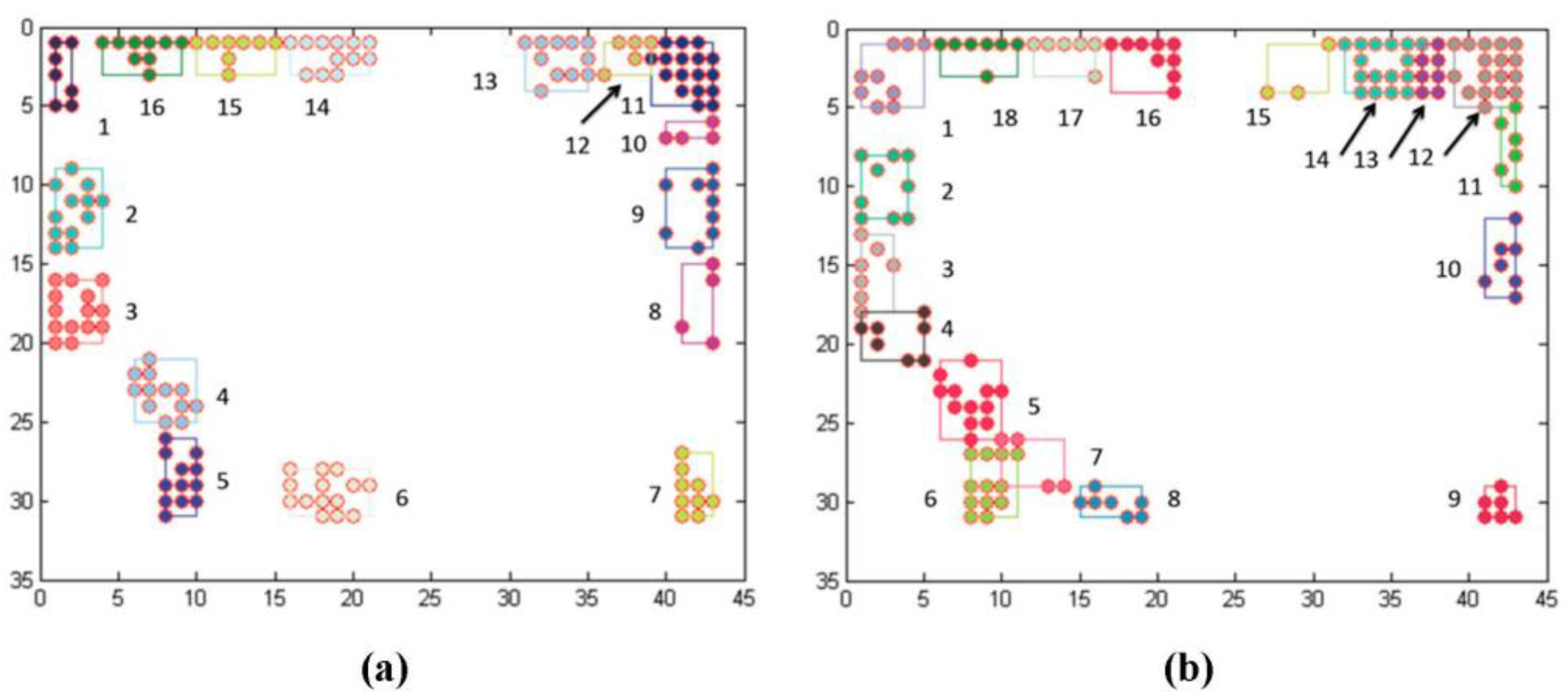
Figure 4. (a) Location of Entrances; (b) and Exits. Entrance and exit locations are identified from trajectory data and their numbers start at top left and move counter clockwise.

Figure 4. (a) Location of Entrances; (b) and Exits. Entrance and exit locations are identified from trajectory data and their numbers start at top left and move counter clockwise.

4.4.2. Sub-Models

There are two specific sub-models that warrant discussion, specifically the way in which gradients are generated based on the source data and the way in which agents plan and accomplish their movement.

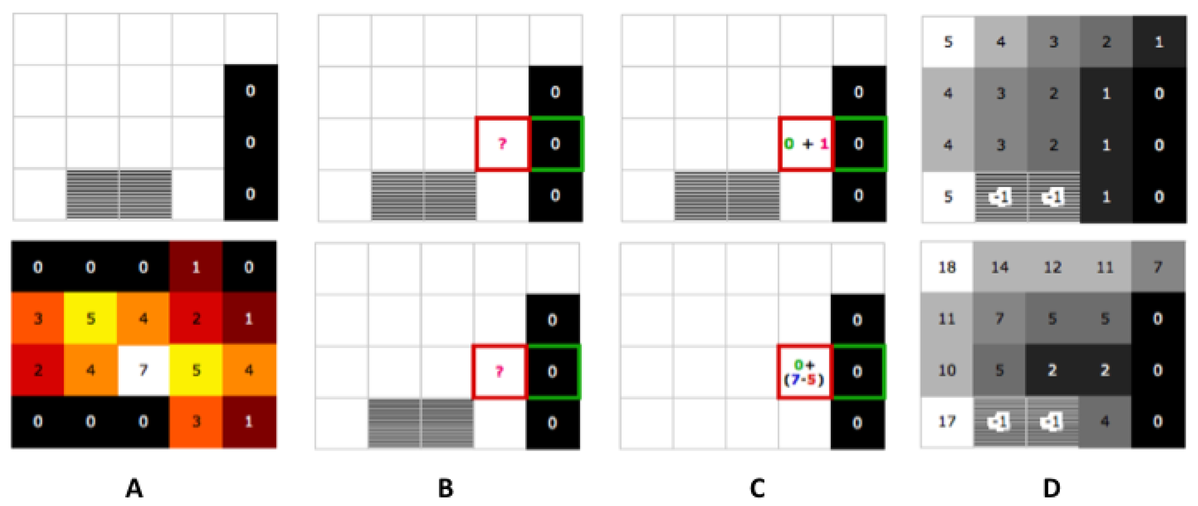
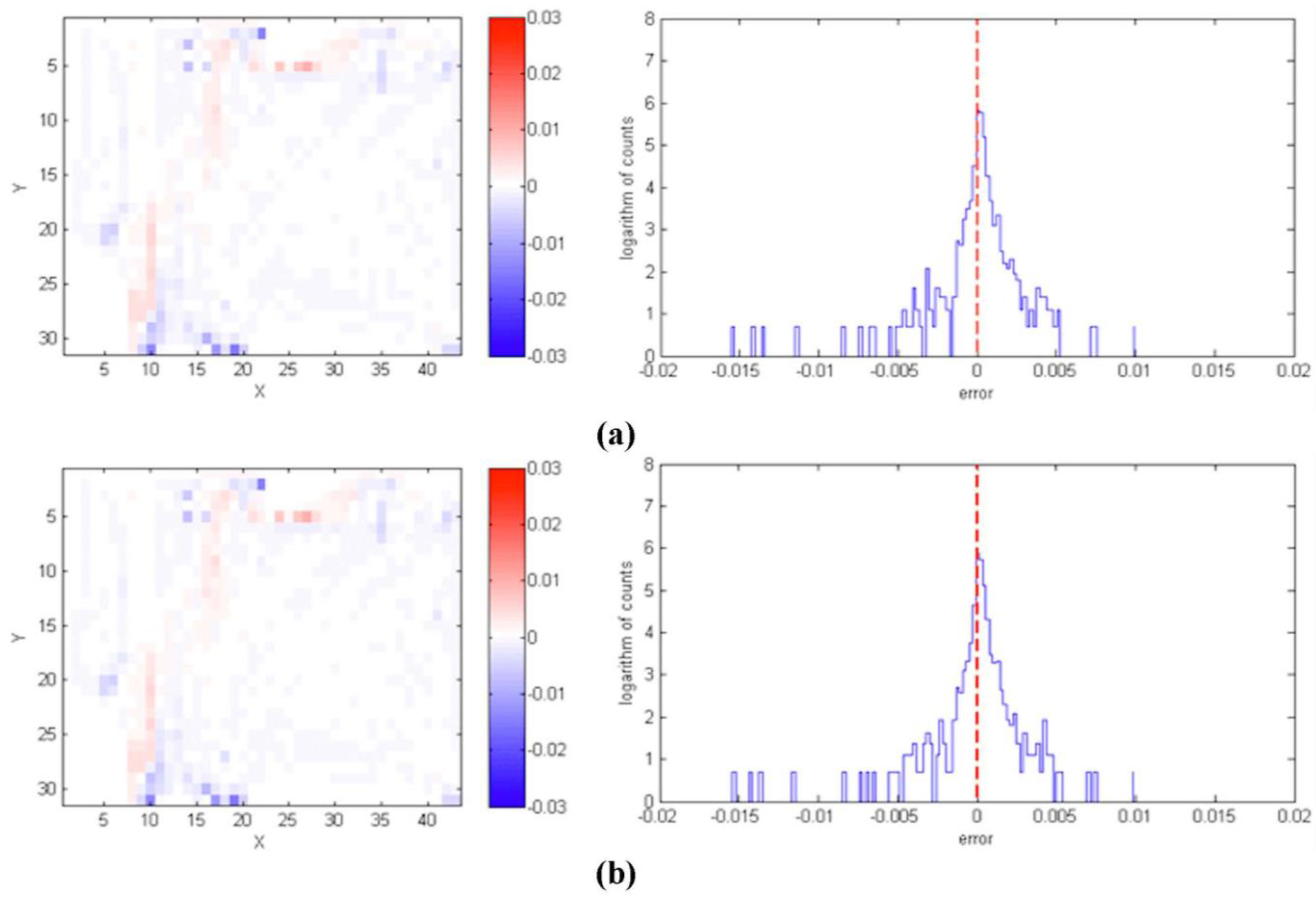
Gradient Production

In the context of this paper, we refer to a gradient as representing a cost in some sense, associated with each entrance-exit pair. Such gradients are commonly used in pedestrian models; see for example [13,18,72]. We chose to consider entrance-exit pairs instead of just exits as entrances contribute a certain scene semantic meaning. For example, a person entering the scene from door 1 and another entering from neighboring door 2 (Figure 4), may be arriving from different parts of the building, and as such they may have different intents and therefore select different exits, even though they me be temporarily spatially proximal. Two kinds of gradients were experimented within this research, specifically one that was calculated solely on Euclidian distances derived from entrance and exit locations (distance-based gradients), and second that was derived from scene activity (activity-based gradients), as shown in Figure 5. For both gradient types, the Moore neighborhood relationship was used in the calculations. For the distance-based gradients, the exit points are assigned a cost of zero, with any locations neighboring the exit points having a distance of zero plus one. Fanning out from these originally tagged locations, further neighboring cells are also associated with the cost of the tagged cell they border plus the cost of moving from that cell to the neighboring cell. In these calculations the transition from one cell to a neighboring cell is assigned to equal one. One can consider this a simple shortest route path that can be computed with Dijkstra’s [81] algorithm. The distance-based gradients also incorporate information about the presence of obstacles, as obstacles are assigned an infinite cost (e.g., a large value), making these cells effectively impassible.

Figure 5. Constructing the gradient for the distance-based (top) and the activity-based heat map (bottom) informed spaces.

Figure 5. Constructing the gradient for the distance-based (top) and the activity-based heat map (bottom) informed spaces.

The activity-based gradients are generated in a similar fashion, with the critical difference that the cost of moving between cells is associated with the corresponding heat map values, as drawn from the CCTV data. The heat map is generated by taking only the paths of agents traveling between the given entrance and exit, and counting the number of times each location is traversed in the data. Based on the resulting heat map, the activity-based gradients are calculated as follows. For each entrance and exit pair, the maximum heat map cell value is found and is used to calculate a difference from all other heat map cells. That value is then assigned as the activity-based gradient for the corresponding cell. One could consider this as an extension of the emergence of trails concept, introduced above but it also relates to work of Golledge and Stimson [82] that showed that via experience of a particular space, people build up a repository of origins and destinations and paths connecting them which don’t have to be the shortest path [83].

These two approaches are shown in Figure 5, in which the top row illustrates process of calculating distance-based gradients and the bottom row shows the process of generating activity-based gradients. In this figure we show four steps in the calculation process, from step A (initialization) to step D (final gradient). In the top row (distance-based gradients), we see the room setup with the exit points marked with cost 0 and the obstacles in the room indicated (step A). In step B, we investigate the points neighboring exit points. In step C, starting from the exit points, we consider the cost of moving from the exit point to the neighbor point. This process of exploring neighboring cells continues, and step D shows the final gradient. In the bottom row, the discovery process is the same, except that the cost of movement between locations is drawn from the heat map shown in the lower row of step B.

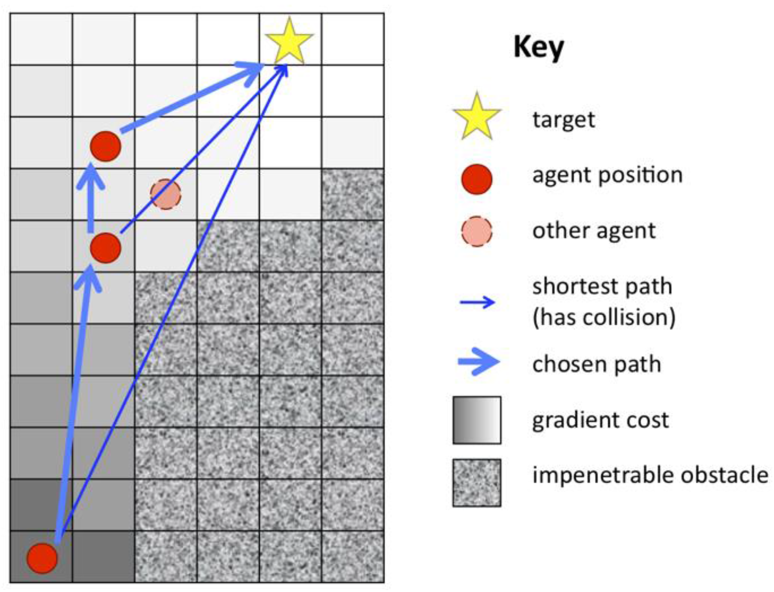
Figure 6. Diagram of the route-planning algorithm.

Figure 6. Diagram of the route-planning algorithm.

Planning Movement

While many navigation methods are possible, including visibility graphs and adaptive roadmaps (see [3,68] for reviews), we are attempting to create the simplest model possible that can produce realistic patterns of pedestrian movement. In order to do so, every time an agent is called upon to move, it performs a number of checks, potentially selects a new intermediate target from among the set of cells it could theoretically reach within the time step, and then moves toward that intermediate target at the maximum possible speed. The checks which can prompt a reassessment of the agent’s intermediate target include whether the agent has reached its current intermediate target point, whether the point is both near and currently occupied, whether the agent is technically moving up the gradient in approaching the point, or whether the agent lacks a clear line of sight to the point. Figure 6 sketches out this process. If any of these are the case, the agent searches to the extent of its vision for the minimum unoccupied gradient point, discarding points that do not have line of sight. This point is taken as the new intermediate target point. Given an intermediate target point, the agent determines its ideal heading. The agent moves to the available cell with the greatest dot product with the heading, selecting the cell with the lowest gradient value in the event that multiple such locations exist.

5. Experiments

In line with ABM practice the built model was verified with respect to its logical consistency to ensure that there were no logical errors in the translation of the model into code, nor any programming errors. This verification was conducted through code walkthroughs, profiling and parameter testing; it ensured that the model behaved as it was intended and matches its design.

Assessing the performance of an ABM comprises two tasks, which in the context of this paper we will refer to as precision and accuracy. The precision of the ABM refers to the degree to which its output matches the data that were used to calibrate it. Inherently an ABM represents an abstraction of the original dataset, and therefore the question that arises is how well does the output of this abstraction match the full dataset? Regarding its accuracy, the challenge is to assess the degree to which such a model would predict actual events for which no data are available (e.g., bridging a gap in our data feed, or predicting a future event). In order to assess the performance of our SA²-ABM approach we present experiments addressing these metrics in Section 5.1 (precision) and Section 5.2 (accuracy). It should be noted here that our assessment is performed at the aggregate scene level: we compare simulation-derived heat maps to the one reflecting the input dataset, in order to stimulate how well our model simulates traffic flow patterns over time in the scene. If one were interested in assessing particular paths within the scene, one could consider using trajectory comparison metrics e.g., employing simple distance-based approaches (such as Hausdorff of Hidden Markov Models), or more complex similarity measures such as the longest common subsequence (LCSS, [84]) and dynamic time warping (DTW) distances, to name but few. Zhang et al. [85] and Morris and Trivdei [86] have presented comparative studies of popular trajectory comparison techniques. However, such trajectory-by-trajectory comparison is beyond the scope of this paper, and is not addressed here.

5.1. Precision Assessment: Scenario Testing

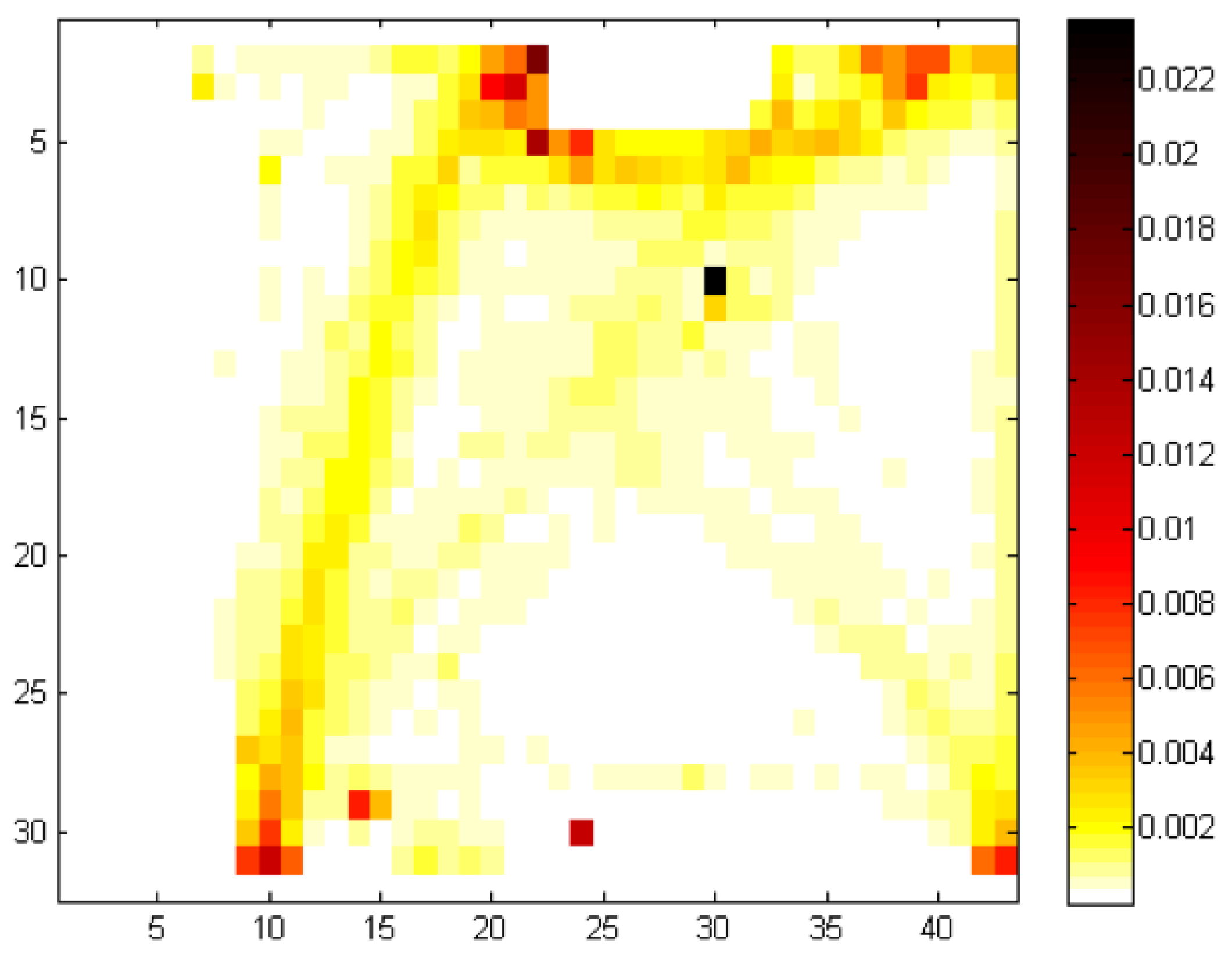
Figure 7 shows the actual normalized heat map generated by foot traffic data collected over 15 h (the whole day) on the 25th of August. This serves as our reference, i.e., the so-called “ground truth” dataset. In our studies we will compare all our simulation results to this reference heat map in order to assess how well the ABM is performing This heat map has been normalized by taking all of the cells traversed and then dividing them by total number of people entering the scene during that day. Regarding its precision, we generated simulations over the same 15-hour time period at one second intervals. In each scenario, the model was run 30 times and we compared the resulting average simulated heat maps to the reference one, in order to assess the precision of the model.

Figure 7. A normalized heat map for the 25th of August, as derived from trajectory data for that date.

Figure 7. A normalized heat map for the 25th of August, as derived from trajectory data for that date.

Scene-specific data can be used to calibrate the ABM, infusing it with knowledge about the particularities of the given scene. In order to assess the effects of various types of calibration data on the precision of the ABM we have chosen to explore four different scenarios, which build upon each other and are detailed below:

• Scenario 1: No Realistic Information about Entrance/Exit Probabilities or Heat Maps

  • In this scenario, entrance and exit locations are considered known, but traffic flow through them is considered unknown. Under such conditions, we run the model to understand its basic functionality without calibrating it with real data about entrance and exit probabilities, nor activity-based heat maps. This will serve as a comparison benchmark, to assess later on how the ABM calibration through such information improves (or reduces) our ability to model movement within our scene.
• Scenario 2: Realistic Entrance/Exit Probabilities But Disabled Heat Maps

  • In this scenario, we explore the effects of introducing realistic entrance and exit probabilities on the model. The heat map models used are distance-based, and not informed by the real datasets. Instead, we use distance-based gradients (i.e., agents choose an exit and walk the shortest route to that exit as discussed in Section 4.4.2).
• Scenario 3: Realistic Heat Maps but Disabled Entrance/Exit Probabilities

  • In this scenario we introduce real data-derived heat maps in the model calibration. These activity-based heat map-informed gradients are derived from harvesting the scene activity data, however entrance and exit probabilities are turned off. In a sense one could consider this a very simple form of learning how agents walk on paths more frequently traveled within the scene. It also allows us to compare to extent to which the quality of the results are due to the heat maps versus entrance and exit probability.
• Scenario 4: Realistic Entrance/Exit Probabilities and Heat Maps Enabled

  • In the final scenario we use all available information to calibrate our ABM, namely, the heat map-informed gradients and entrance-exit combinations and see how this knowledge impacts the performance of the ABM.

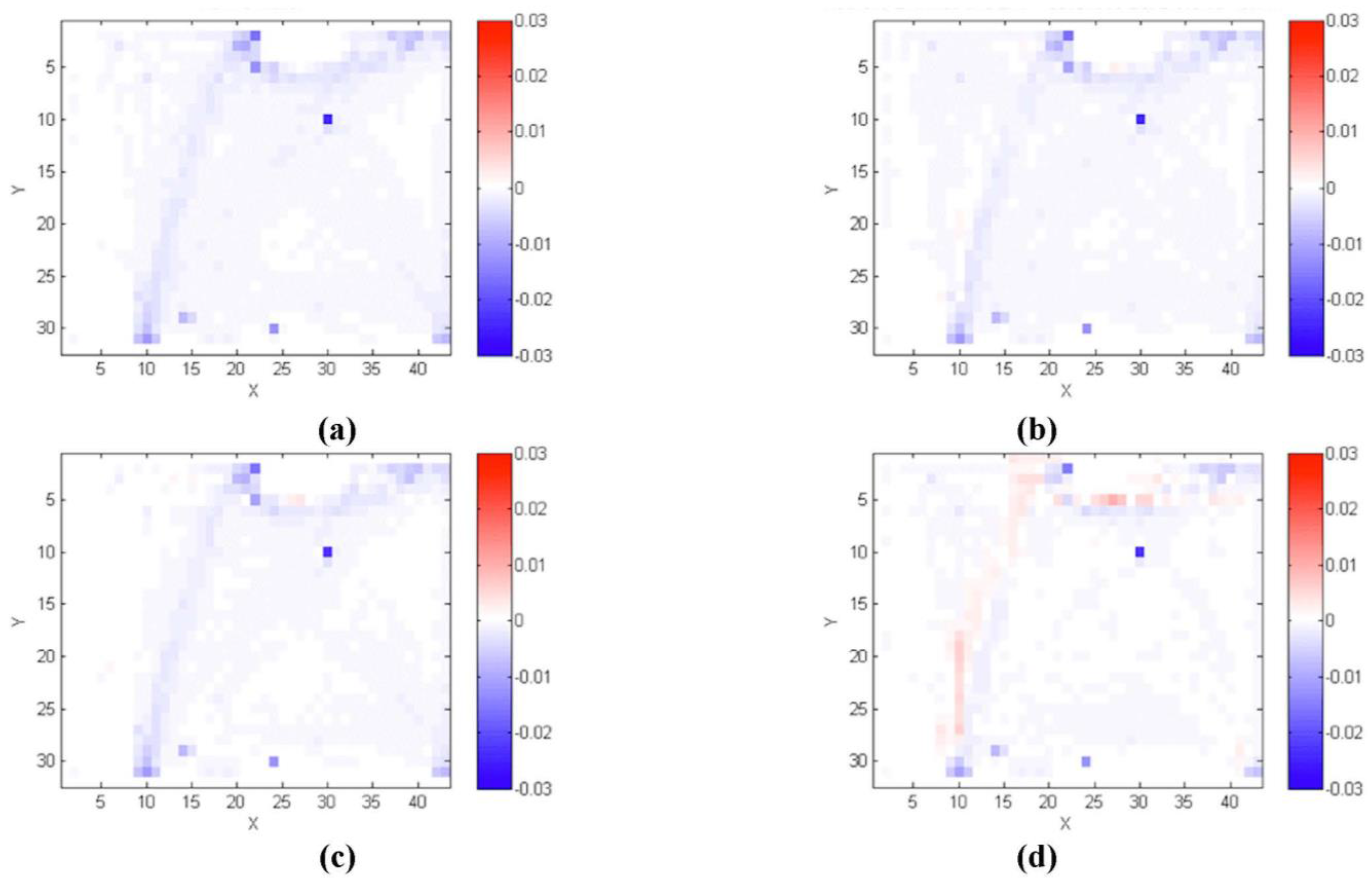
Figure 8. Normalized heat maps comparing a specific simulation scenario with the actual data. (a) Scenario 1: No realistic information about entrances, exits, or heat maps; (b) Scenario 2: realistic entrance/exit probabilities but disabled heat maps; (c) Scenario 3: realistic heat maps but disabled entrance/exit probabilities; (d) Scenario 4: realistic entrance/exit probabilities and heat maps enabled.

Figure 8. Normalized heat maps comparing a specific simulation scenario with the actual data. (a) Scenario 1: No realistic information about entrances, exits, or heat maps; (b) Scenario 2: realistic entrance/exit probabilities but disabled heat maps; (c) Scenario 3: realistic heat maps but disabled entrance/exit probabilities; (d) Scenario 4: realistic entrance/exit probabilities and heat maps enabled.

Figure 8 shows a comparison of the four scenarios with those generated by actual real pedestrian paths (For the comparison of the real data and the simulated data we took all 30 runs from each of the scenarios and then summed up each cells usage value and divided them based on total number of steps all the agents made during the 30 runs. This normalized heat map was then compared to the normalized heat map of the real data). The scale bar for all the scenarios in Figure 8 goes from red to blue, with darker red showing over-predicting and darker blue showing under-predicting. White shows a perfect match of the model with the data. Even the simple experiment (Scenario 1) demonstrates simple emergent phenomena as agents interact with their environment and each other to develop paths over time. What is clear from this scenario is that with no other information, the ABM is under-predicting actual traffic. This is evident in Figure 9 which shows the difference between over- and under-predication in each of the scenarios where the Y axis is the log of the number of pixels having a given error value from the heat map comparison.

Figure 9. Bar charts of a specific simulation scenario comparing the difference between the average simulation output and the actual data. (a) Scenario 1: No realistic information about entrances, exits, or heat maps; (b) Scenario 2: realistic entrance/exit probabilities but disabled heat maps; (c) Scenario 3: realistic heat maps but disabled entrance/exit probabilities; (d) Scenario 4: realistic entrance/exit probabilities and heat maps enabled.

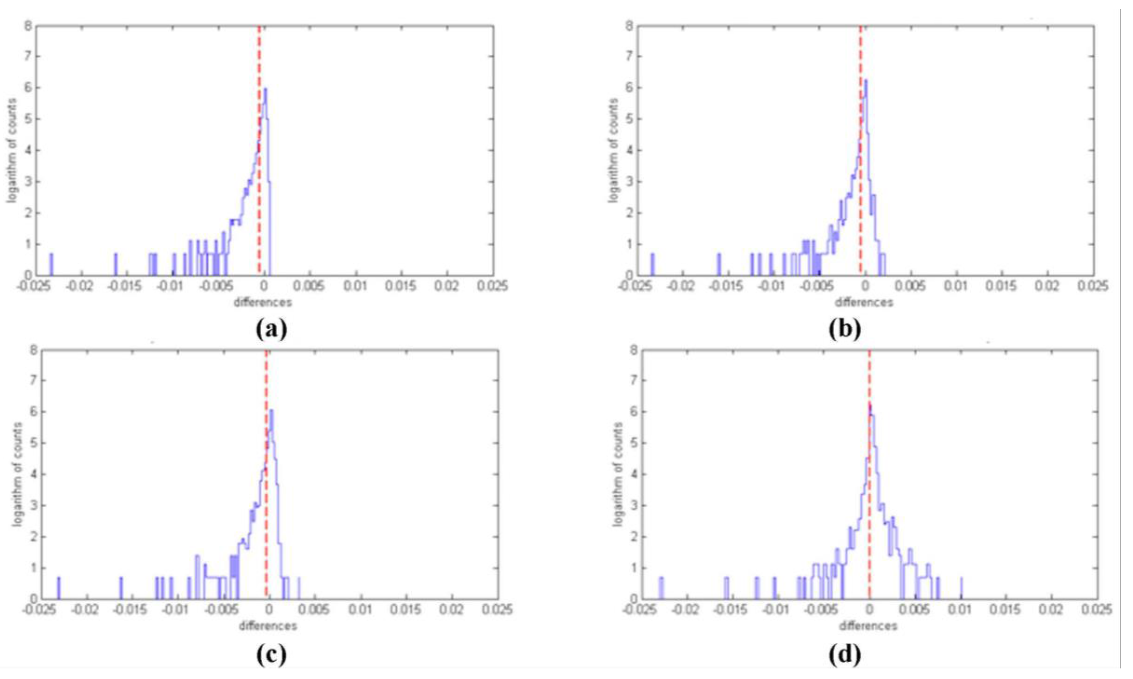
Figure 9. Bar charts of a specific simulation scenario comparing the difference between the average simulation output and the actual data. (a) Scenario 1: No realistic information about entrances, exits, or heat maps; (b) Scenario 2: realistic entrance/exit probabilities but disabled heat maps; (c) Scenario 3: realistic heat maps but disabled entrance/exit probabilities; (d) Scenario 4: realistic entrance/exit probabilities and heat maps enabled.

Table 3 shows the summary statistics for the errors of each scenario (In addition to this test we also found that different neighborhood types (e.g., Moore, von Neumann, Hamiltonian) made little difference on the simulation outcome). Here we define error as the simulation results minus the true heat map. While in all scenarios the standard deviation of the error and the maximum absolute difference remain roughly the same, this is not the case for the mean error and the skewness, which drops considerably in scenario 4. For example, the mean error drops an order of magnitude, from −0.000533 in scenario 1 to 0.000062 in scenario 4 while the skewness drops similarly from −7.17441 to −4.72599. From the examination of the other scenarios we can see that by adding further information into the SA²-ABM the model starts matching the ground truth more, and therefore the accuracy of the SA²-ABM is improving.

A smaller mean error value as we progress from scenario 1 to 4 implies a reduced bias. As can be seen from the results, without incorporating both entrance and exit information and the heat maps the model is still under-predicting paths between entrances and exits. This could be explained by the fact that without realistic entrance-exit selection, people will walk less on paths that are objectively more frequently traveled and more on infrequently traveled paths, smoothing the overall usage statistics. Without any scene-specific information, the ABM would have its pedestrians traversing the scene following the shortest path connecting an entrance and an exit, thereby producing a lower number of total number of steps in the scene compared to reality, the predominate blue colors in Figure 8a–c. However, when incorporating scene-specific information, one can see how the model avoids this bias, producing balanced errors, and this can be explained by the route-planning of the ABM. In all of the scenarios we are under-predicting in many of the same places (e.g., X30, Y10 and X24, Y30 and X10 Y32 and X14 Y29 of Figure 8). Looking back to the scene activity information, these areas have the highest traffic (as shown in Figure 7), but also mark areas of entrances and exits; this relates to how the scene information is being captured. People are recorded every second they are in the environment, so that if they pause or meet someone at a specific location, this increases the weight of that cell. In the ABM, agents only have simple behavior to navigate throughout the scene as quickly as possible and to avoid obstacles. The argument we make here is that this shows that there are some fine dynamics with entering and exiting the space (such as jostling at the door) that the video does catch but the SA²-ABM does not. This behavior / discovery will be a point of further work.

Table 3. Summary statistics from the different scenarios.

Scenario	Mean of Error	Standard Deviation of Error	Max Absolute Difference	Max Count	Value of Max Count	Skewness
No information	−0.000533	0.001390	0.023400	398	0.000036	−7.17441
Realistic entrance and exit probabilities but disabled entrance-exit probabilities	−0.000458	0.001310	0.023400	516	−0.000020	−7.9975
Heat maps enabled but disabled entrance-exit probabilities	−0.000334	0.001370	0.023200	425	0.000097	−7.31764
Both realistic entrance-exit probabilities and heat maps enabled	0.000062	0.001430	0.023000	501	−0.000070	−4.72599

Table 3. Summary statistics from the different scenarios.

Scenario	Mean of Error	Standard Deviation of Error	Max Absolute Difference	Max Count	Value of Max Count	Skewness
No information	−0.000533	0.001390	0.023400	398	0.000036	−7.17441
Realistic entrance and exit probabilities but disabled entrance-exit probabilities	−0.000458	0.001310	0.023400	516	−0.000020	−7.9975
Heat maps enabled but disabled entrance-exit probabilities	−0.000334	0.001370	0.023200	425	0.000097	−7.31764
Both realistic entrance-exit probabilities and heat maps enabled	0.000062	0.001430	0.023000	501	−0.000070	−4.72599

Nevertheless, the above scenarios have demonstrated how we can gain some sense of validity with our model, namely where we are able to compare the output from the individual interactions and compare it to aggregate data collected from the real-world. In a sense one could consider these scenarios as a method of calibration, fine-tuning the model to a particular dataset. However, this is not calibrating specific agent parameters (such as movement rules, walking speeds etc.) but giving the agents more information on which to make their routing decisions.

5.2. Accuracy Assessment: Activity Forecasting

An essential goal of agent-based modeling (and modeling in general) is the ability to forecast activities in order to carry out what if scenarios. Here we carry out two such scenarios, specifically “how well can we simulate missing data?” and “can we forecast the effect of added obstacles in the patterns of movement in the scene?” Given our data availability, the first scenario serves as an assessment of the accuracy of the model (as we will be comparing simulated data to actual information, as we will see later in this section), whereas the second scenario serves as a demonstration of the model’s potential.

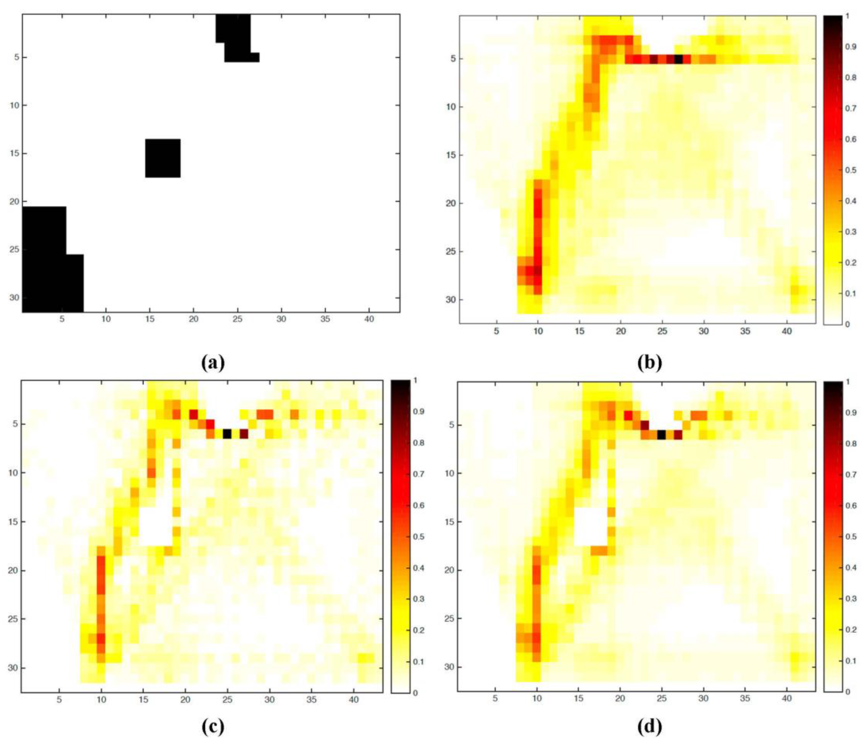
Regarding the first example, the practical challenge that we are addressing is how well we can reconstruct a scene activity with our SA²-ABM if the system experiences a power outage and goes down for one hour. In order to explore how well movement patterns could be extrapolated from limited data, we created artificial data gaps by removing all data recorded between 8 a.m. and 9 a.m., one of the highest-traffic hours, from the record for August 25th. This set of points is indicated in Figure 10a, and their omission effectively imitates a sensor failure. Constructing the heat maps and entrance/exit probability distributions from this limited dataset, we attempted to recreate a realistic projection of what the missing hour of data might have looked like. In Figure 10b we show the actual heat map between 8 a.m. and 9 a.m., which was not used in the experiment but instead was later used as a reference dataset to assess the accuracy of our simulation results. We use the heat map generated throughout the day, excluding only the information collected between 8 and 9 a.m., as our heat map to guide agent movement. We then ran two experiments, one where the number of agents between 8 a.m. and 9 a.m. is known (but not their entrance and exit probabilities) and the second where agents were randomly generated (that is, agents were generated based on the distributions drawn from the rest of the day). Figure 11 compares our results with the actual use patterns during the missing hour. Our success in predicting the general flow of traffic is particularly interesting in light of the fact that usage patterns can differ across the day, the morning rush displaying different characteristics than the lunch crowd or the peregrinations of janitors during the quieter periods of the day. Despite the fact that we left data from the busiest period of the day out of the model, our projections of use patterns line up nicely with the reality, as shown in the summary statistics of Table 4.

Figure 10. Scene Information (a) Distribution of people through the scene over time; (b) The actual heat map of traffic from 8 a.m.–9 a.m.

Figure 10. Scene Information (a) Distribution of people through the scene over time; (b) The actual heat map of traffic from 8 a.m.–9 a.m.

In the second scenario, we use the model we have constructed to project how pedestrians would respond to new circumstances. Specifically we use the model to predict how agents would react in the face of a changing environment, as may be the case when a large obstacle (e.g., a piece of artwork or furniture) measuring 2 m by 2 m is installed in the middle of a major pathway (Location X = 13 Y = 15). By modifying the layer representing stationary obstacles in the environment, we introduced a situation where individuals had to balance avoidance of elements of the environment with the normal patterns of movement as shown in Figure 12a. In addition we also assess the performance of the model under heavy traffic conditions, we generated in this scenario a situation with 30 pedestrians in the scene at any one time (We could have added more pedestrians in the scene but at greater numbers, such as 60 agents in the scene at any one time leads to bottlenecks forming around exits (i.e., doors)). The probability of entrance and exit selection is unchanged: pedestrians are merely added to the simulation more frequently. This makes the assumption that the number of pedestrians using the space increases without their door selection patterns varying.

Figure 11. Comparison of the two experiments against the real data. (a) Agents generated from the actual counts between 8 a.m. and 9 a.m.; (b) Agents generated from the data for the rest of the day.

Figure 11. Comparison of the two experiments against the real data. (a) Agents generated from the actual counts between 8 a.m. and 9 a.m.; (b) Agents generated from the data for the rest of the day.

Figure 12b shows the results of just increasing the number of pedestrians in the scene, without additional obstacles. This is similar to Figure 7 and Figure 8, suggesting that the model can handle more traffic. The introduction of obstacles leads to more interesting observations. Figure 12c,d show the resulting heat maps as the agents are avoiding this newly introduced obstacle. Figure 12c shows the results of an average traffic situation (same settings as in Section 5.1), while Figure 12d shows the results of high traffic volumes. In all three cases (Figure 12b–d), the agents are initialized with realistic entrance and exit probabilities and also informed by the canonical heat maps. By adding additional pedestrians into the scene, more space was utilized (i.e., 91 more cells (6.6%) were traversed), which is to be expected, as agents not only have to navigate around the obstacle but also around each other. If we compare the situation where no obstacle was added to the scene (Figure 12b) and the one with the obstacle, the obstacle accounted for 20 more cells (1.5%) being traversed.

Table 4. Summary statistics from the two different experiments.

Scenario	Mean of Error	Standard Deviation of Error	Max Absolute Difference	Max Count	Value of Max Count	Skewness
Agents generated from the actual counts between 8 am and 9 am	0.0000706	0.00135	0.0155	340	−0.0000611	−9.48E−17
Agents generated from the data for the rest of the day	0.0000693	0.00135	0.0154	357	−0.0000493	1.76E−17

Table 4. Summary statistics from the two different experiments.

Scenario	Mean of Error	Standard Deviation of Error	Max Absolute Difference	Max Count	Value of Max Count	Skewness
Agents generated from the actual counts between 8 am and 9 am	0.0000706	0.00135	0.0155	340	−0.0000611	−9.48E−17
Agents generated from the data for the rest of the day	0.0000693	0.00135	0.0154	357	−0.0000493	1.76E−17

Figure 12. (a) Obstacles (black squares) added to the scene; (b) Heat map of increased traffic without obstacle; Normalized heat maps for low (c) and high (d) volumes of pedestrian traffic following the introduction of the obstacle for the 25th of August.

Figure 12. (a) Obstacles (black squares) added to the scene; (b) Heat map of increased traffic without obstacle; Normalized heat maps for low (c) and high (d) volumes of pedestrian traffic following the introduction of the obstacle for the 25th of August.

Lacking real data against which to verify these paths, it is impossible to quantify how accurately our model predicts what the true paths would be. However, the movement patterns appear realistic and reasonable in the sense that agents take different paths around the obstacles and emulate the patterns of movement from previous experiments. To paraphrase Mandelbrot [87] models that generate spatial or physical predictions that can be mapped or visualized must “look right”; our model meets this qualitative evaluation. This suggests that the methodology could help planners quickly recalculate the parameters of normal movement through the space. This is one of the reasons for using agent-based models: in areas where data is lacking, absent, or unobtainable, we can experiment with what if scenarios once we have confidence in the basic model structure and dynamics.

6. Outlook

As discussed in the introduction, traditional pedestrian ABMs have been lacking grounding onto real datasets. This has been a reflection of the composite challenge of collecting and analyzing large amounts of such data. As big trajectory data are becoming more readily available to our community we are now at a position where we can leverage such information to build more precise and accurate geographically-explicit pedestrian models. In this paper we introduced an approach to use real scene mobility information to improve the performance and accuracy of a pedestrian ABM, producing a Scene- and Activity-Aware ABM (SA²-ABM). We see this as an essential step towards further bridging the current gap between the agent-based modeling and the geoinformatics communities.

Specifically, we have demonstrated that when using a standard ABM without any scene information the performance of the model may vary considerably, which limits its utility for analysis and prediction. This is remedied by adding scene information, and specifically using entrance and exit probabilities, and/or activity summarizations in the form of heat maps of that scene. While each piece of information singlehandedly improves the basic ABM, it was their combination that improved it the most. The improvement can be seen as a reduction of mean error and skewness. Simply put, the SA²-ABM simulation is a better approximation of reality than just a simple ABM lacking scene information.

The proposed approach takes advantage of the proliferation of video surveillance technologies, by harvesting activity information from video-derived trajectories and using it to inform an ABM for the depicted scene. By doing so we gain substantial and non-trivial knowledge about the depicted scene, recognizing for example important patterns of activity, and gaining a greater understanding on how humans use the scene in everyday life. This allows us to move beyond simply exploring the scene geometry (i.e., the form of the scene) to taking into account the scene’s function as it is reflected through the patterns of movement in that scene.

This work can also be extended in the future to actively support video surveillance, rather than simply feeding on its results. Firstly, the activity models that are generated for an area through the approach we described in this paper can be used to extrapolate human activities for the gap areas in-between neighboring surveillance fields of view. Thus, the movement of a person tracked in one camera as part of a system of non-overlapping video feeds can be extrapolated using the corresponding SA²-ABM to predict where that person is heading and estimate the camera in which he/she will be appearing next.

Furthermore, the SA²-ABM can be used to provide reference baselines for future video feeds in a scene, supporting the detection of unusual activity as deviations from this model. Having a profile of movement relative to some baseline can help us explain and identify deviance when it occurs. Both of these emerging opportunities highlight the evolving nature of pedestrian modeling, which is transitioning from simple simulation support to a valuable tool for describing real and anticipated activities in a scene. More generally, with respect to geographically explicit agent-based models, we can explore human-like behaviors that the data alone cannot provide [23]: motion capture/surveillance equipment alone will not tell us what might happen if an obstacle was placed in the center of the scene or a door was blocked, while an agent-based model could. Furthermore, by modeling the individual pedestrians in space and time, we can explore how basic assumptions or ideas about how one utilizes their spatial environment can be played out within a computer simulation and compared with scene information to determine whether these patterns are seen in the real-world.

Given the wide variety of urban spaces and activities within them, along with the emergence of diverse new sources of tracking data, this contribution should be viewed as a first step towards future explorations, rather than as a final product. This is one reason why we provide the source code and data: for other researchers to explore the model in different situations if they so desire. Furthermore, the model itself can become more complex through the introduction of additional parameters or by exploring other techniques such as machine learning or different cognitive frameworks (see [88]) for agent behaviors allowing for example the incorporation of complex activities such as stopping to talk to people, jostling around entrances and exit points. By showing that even a relatively simple geographically explicit agent-based model like SA²-ABM can replicate the main patterns of a dynamic scene we have demonstrated the huge potential of this approach for the emerging opportunities presented through the coupling of agent-based models with spatiotemporal data.