HybVOR: A Voronoi-Based 3D GIS Approach for Camera Surveillance Network Placement

Abstract

As a consequence of increasing safety concerns, camera surveillance has been widely adopted as a way to monitor public spaces. One of the major challenges of camera surveillance is to design an optimal method for camera network placement in order to ensure the greater possible coverage. In addition, this method must consider the landscape of the monitored environment to take into account the existing objects that may influence the deployment of such a network. In this paper, a new Voronoi-based 3D GIS oriented approach named “HybVOR” is proposed for surveillance camera network placement. The “HybVOR” approach aims to achieve a coverage near 100% through three main phases. First, a Voronoi Diagram from buildings’ footprints is generated and cameras are placed on the Voronoi Edges. Second, the level of coverage is assessed by calculating a viewshed based on a raster Digital Surface Model of the region of interest. Finally, the visibility of the main buildings’ entrances is evaluated based on a 3D vector model that contains these features. The effectiveness of the “HybVOR” approach is demonstrated through a case study that corresponds to an area of interest in Jeddah Seaport in the Kingdom of Saudi Arabia.

1. Introduction

Demand for security and surveillance technologies has emerged recently. This kind of technology provides potential solutions for preventing and reducing crimes and violations. With this significant demand, the use of camera surveillance networks has increased. Indeed, camera or video surveillance is considered as a powerful system used in maintaining order and security in public space (such as transport infrastructure, seaport, airport, parks, stores, etc.). Accordingly, it is necessary to define appropriate and optimal methods that determine the best location of cameras surveillance.

In fact, Camera Placement has a strong effect on the quality and the efficiency of surveillance. An appropriate placement is related to camera properties such as; the range, the field of view, the resolution, the cost of use, the type of the camera (visible-light, infrared…) and so on. However, the most important factor is the environment in which the placement will take place. Indeed, the effectiveness of video surveillance system depends heavily on the physical placement of cameras [1].

Seaports are among the most important places where security is a major concern. Indeed, they are one of the most essential facilities for commercial and tourism activities, especially for coastal countries. They play a major role in the worldwide merchandises’ distribution because almost 90% of these goods are shipped through maritime port [2]. Hence, in recent decades, the need for improving seaports security is growing in order to allow safe and efficient transportation of people and merchandises through these transit hubs [3]. In general, the main issues related to seaport security may be classified as perimeter security, internal security and operative controls, maritime security, port community systems, decision support systems, prevention and emergency management, etc. [4]. To deal with these issues, there are many useful technologies such as video surveillance, radar and sonar, cargo/container screening systems, perimeter security systems, mass notification, wireless systems [3]. According to the same reference, video surveillance is the most common technology used for port security. Through analytic methods, it is possible to extract very useful information from the acquired videos such as perimeter intrusion, following object of interest, and object classification [3]. However, the complexity of the physical landscape can make the tasks of monitoring seaports very hard to fulfill [3].

In this paper, a new GIS oriented approach called “HybVOR” (Hyb: Hybrid, VOR: Voronoi) is proposed. It aims to find the optimal placement of surveillance cameras. The main purpose is to reach coverage close to 100% with a minimum number of cameras. The proposed approach is based on a combination of: (1) 3D Modelling and analysis of the Seaport physical landscape and (2) Voronoi approach for the segmentation of space. The space segmentation based on Voronoi Diagram will allow us to specify the number and the location of the cameras for an optimal coverage. In addition, the analysis of the seaport 3D model is based on a combination of Raster and 3D Vector Analysis offered by GIS software, hence, the part “Hyb” (from Hybrid) of the name HybVOR. These two types of spatial analysis allow calculating and assessing the coverage area based on the network placement of the surveillance cameras.

This paper is structured as follows: The first Section is a literature review on surveillance cameras placement, Voronoi diagram principles, and coverage calculation. The second Section is dedicated to, the principles of HybVOR approach. This Section demonstrates why and how this proposed approach combines Raster and Vector 3D analysis with Voronoi Diagrams. Next, a case study that corresponds to the implementation of the HybVOR approach in Jeddah Seaport is introduced. Afterward, a discussion regarding the results of this case study is presented. Finally, the last section concludes this work and highlights some of the important perspectives and future works.

2. Related Works

Sensor placement in general, and particularly cameras, is a research topic that has attracted the interest of several research groups around the world. The main objective of camera placement is defining viewpoint positions in order to pick the most informative views of a scene of interest [5]. The camera placement is related to various issues such as surveillance, tracking and scene monitoring [6], part inspection [4], three dimensional reconstruction and robotic sensor ([1,7]) and the Art Gallery problem [8].

The most intuitive method for camera placement is to place uniformly a camera network in the area of interest. This method may give quite interesting results for a non-complex area where the only issue is maximizing the coverage. However, in most cases, the problem is much more complex and difficult. Indeed, the issue of camera placement may be approached from several perspectives according to the purpose of the system. Accordingly, the camera placement approaches presented in the scientific literature may be classified into two main categories: (1) Target-based approaches and (2) Landscape based approaches.

2.1. Target-Based Approaches

Target-based approaches tend to find the placement of cameras according to a target of interest. The target can be an object, an event or a phenomenon that may evolve in space and time. The target-based approaches focus mainly on the nature of the target rather than focusing on the level of coverage [6].

In [7], the authors propose a method for automatic sensor placement based on 3D CAD data file. The purpose of this method is to find the best viewpoint positions of a vision-sensor with the appropriate parameters such as position, orientation, and optical setting. In addition, each viewpoint has to satisfy some predefined constraints that are mainly related to the physical and optical properties of the sensor. This approach was developed for the field of model-based robot vision. The main goal is to move one sensor (using a robot) from one position to another one around the object to monitor and analyse important features that characterize the studied target. Likewise, there are other similar works related to 3D reconstruction of objects and space such as [9,10,11], etc.

In [6], the authors introduce an analytical formulation to monitor the locomotive motion paths taken by people through a scene of interest. This method focuses on maximizing the observability of the target and capturing its motion. The authors stipulate that their approach requires only a minimum set of a priori knowledge about the target and no a priori knowledge about the physical landscape where the event takes place.

Based on the results of the paper [1,6] have developed a solution that combines fixed and mobile cameras to define the placement of a Surveillance Camera Network. The authors propose to use fixed cameras to observe the entire scene in order to extract the movement of targets (people in this case). Then, this obtained knowledge is used to determine the placement of mobile cameras based on quality criteria which are: Foreshortening, ground coverage, and resolution.

2.2. Landscape Based Approaches

Landscape based methods assume that physical properties of the environment, where cameras placement will take place, are known a priori. This family of methods aims to optimize the coverage area. The definition of coverage is variable from one domain to another [12]. A general definition of coverage is proposed by [13] as the quality of surveillance, which can be provided by a sensor network and how well an area of interest is monitored.

One of the well-studied topics related to landscape based approaches is the Art Gallery Problem [14]. It intends to determine the number of observers (cameras for example) to monitor every point inside a polygon area (Art Gallery Room). In other words, this problem tries to find the optimal number and location of observers within the landscape in order to satisfy the desired coverage or to maximize the coverage ([8,15]).

In the same vein, other researchers propose many discrete optimization methods for sensor placement. A genetic algorithm methodology to optimize sensor placement was proposed in [16]. An approach based on a parallel evolutionary optimization technique to choose and order candidate sites for sensors was developed in [17]. Another work presented in [18] aims to place sensors based on Simulated Annealing technique to find the best configuration of the network. All these three methods were applied on very simplest environments that do not reflect the complexity and the diversity of real landscapes.

A Voronoi based algorithm was developed in [19] that integrates a Digital Surface Model of the area of interest. This Algorithm was inspired from the work of [20] which proposes three Voronoi strategies: (1) Vector-Based (VEC), (2) Voronoi-Based (VOR) and (3) Minimax. The authors in [19] propose first to generate a Voronoi Diagram from an initial position of sensors. Then, the sensor network is optimized by moving each sensor towards its farthest Voronoi vertex until reaching the highest elevation inside the Voronoi Cell. Likewise, a research work proposed by [21] combines a probabilistic sensing model with a Digital Surface Model to define the optimal placement of sensor network. This probabilistic sensing model consists of membership functions based on sensing range and sensing angle.

It is important to mention that these latest two algorithms, which integrate the landscape reality through a Digital Surface Model, use the line of sight method in order to determine the percentage of coverage. When combined with a Digital Surface Model (or a Digital Terrain Model), the line of sight method is a very effective way for surveillance camera placement, because it allows introducing some important characteristics of cameras such as the 3D position of each camera, observation azimuth, field of view, the range of the camera, etc. (Please refer to Section 3 for more details).

2.3. Discussion

The choice of an appropriate deployment method of a camera network depends strongly on the aim of each system. In fact, target based methods are more suitable for monitoring specific objects that may move in the monitored environment, while the goal of landscape based methods is to maximize the coverage area in order to observe the whole scene of interest. The main objective of this paper is to propose a novel method that belongs to the landscape based approach. Our proposed method is also based on the space segmentation using Voronoi Diagram (as the works of [19,20,21]). However, as detailed in the following sections, the proposed solution differs from other methods found in the literature in two fundamental aspects: (1) the choice of objects that generates the Voronoi Diagram and (2) The method of assessing the level of coverage.

On one hand, Voronoi-based methods that are presented in previous work ([19,20,21]) use the expected position of the sensors (cameras) to generate the Voronoi diagram. Each Voronoi cell will contain the objects of the environment that may be monitored by the corresponding sensor. However, it will be more judicious to start by analyzing the environment where the sensor deployment will take place, and then propose the optimal position of the sensors based on the result of such analysis. For this purpose, the Voronoi Diagram will be generated based on objects of interest (i.e., Buildings) that exist in the monitored environment. Thereafter, cameras will be placed initially on the edge of each Voronoi cell.

On the other hand, the methods that integrate a model of the area of interest when calculating the coverage use either a very simplistic model ([16,17,18]) or a Digital Surface Model (DSM) that represent only the surface of the monitored environment ([19,21]). This second category allows only assessing the coverage level of the surface that can be seen from above. Nevertheless, it is impossible through these methods to assess the visibility of vertical surfaces that may be very important to monitor such as walls, doors, windows, etc. Hence, it is important to combine the visibility assessment based on raster DSM with 3D models that takes into consideration all facets (surface and vertical) of objects in the environment of interest.

In the following sections, a recall about the main principles of Voronoi diagrams, as well as the coverage calculation are presented. Thereafter, the proposed approach called “HybVOR” for deployment of surveillance cameras is detailed.

3. Coverage Calculation Based on the Line of Sight

The concept of coverage reflects how well an area is monitored by a set of sensors [22]. The coverage problem has been investigated in the scientific literature based on several approaches, depending on the nature of the application. One example is the art-gallery problem that aims to define the required number of cameras where each point in the gallery is covered by at least one observer [22]. In the art-gallery problem, the coverage is defined by the direct visibility between the observer and the target [23]. Another example related to coverage issues is extending the lifetime of sensors through reducing energy consumption ([24,25,26]). These approaches try to identify and turn off the redundant sensors that cover the same zone when their use is not gainful.

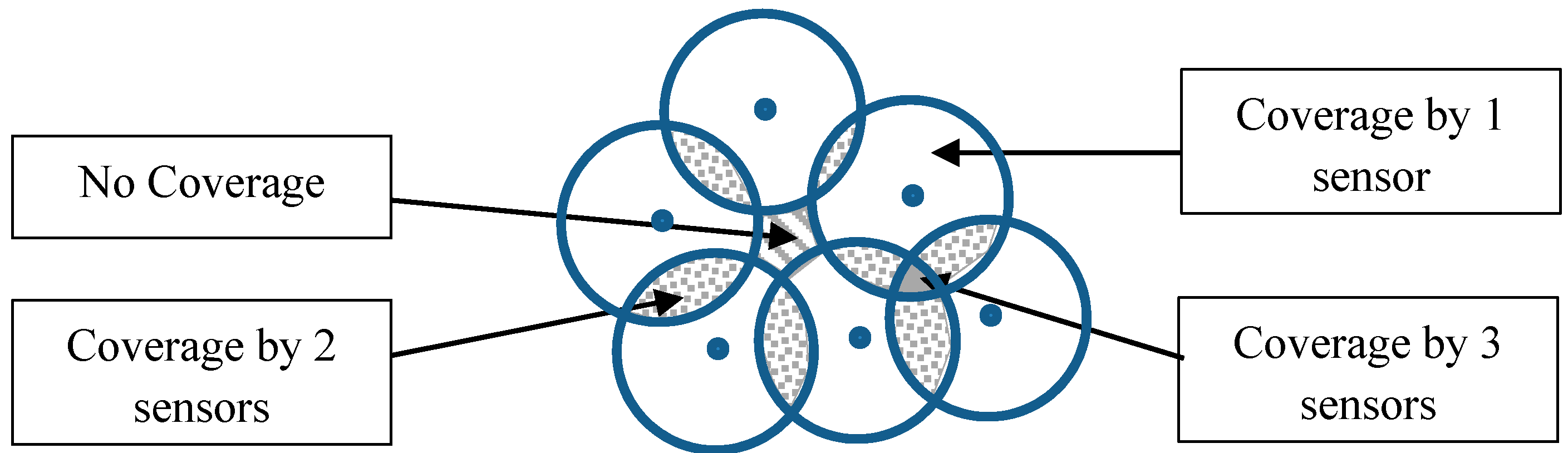
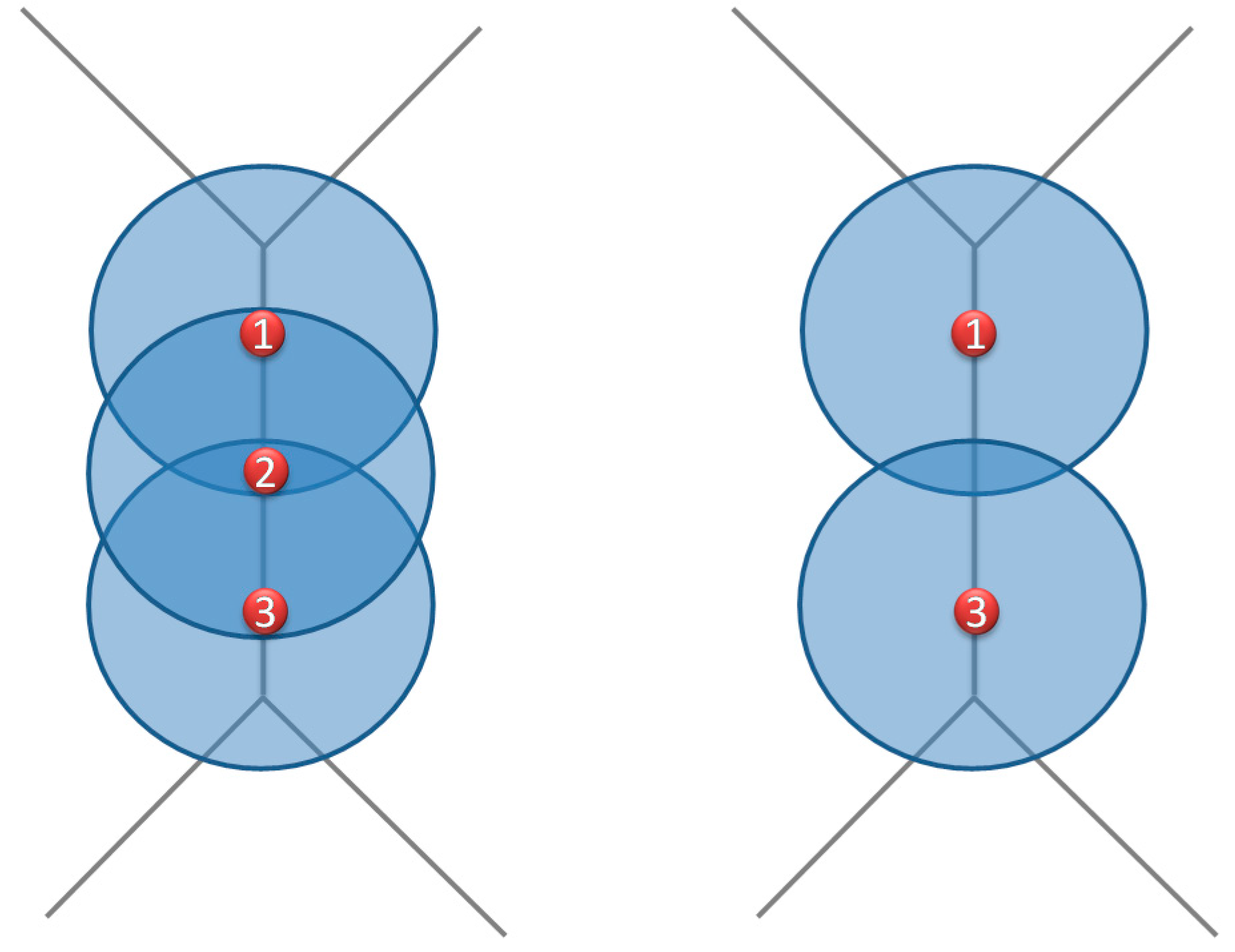
A general definition of the coverage problem was proposed by [22], it stipulates that for a given set of sensors deployed in a target area, every point in the zone of interest is covered by at least k sensors, where k is the number of sensors that monitor simultaneously the target. In Figure 1, the white circle corresponds to the area covered by one sensor, the dotted zones correspond to areas covered by two sensors, the gray zone corresponds to the area covered by three sensors, and the dashed zone corresponds to a non-covered area.

Figure 1. Coverage areas generated by a set of sensors.

Figure 1. Coverage areas generated by a set of sensors.

The coverage is mainly related to the sensing range of each sensor, which is related to the monitored phenomenon, and the obstacles that exist in the target zone. Hence, developing a model that allows calculating the coverage must take into consideration the nature of the application and the presence of obstacles. 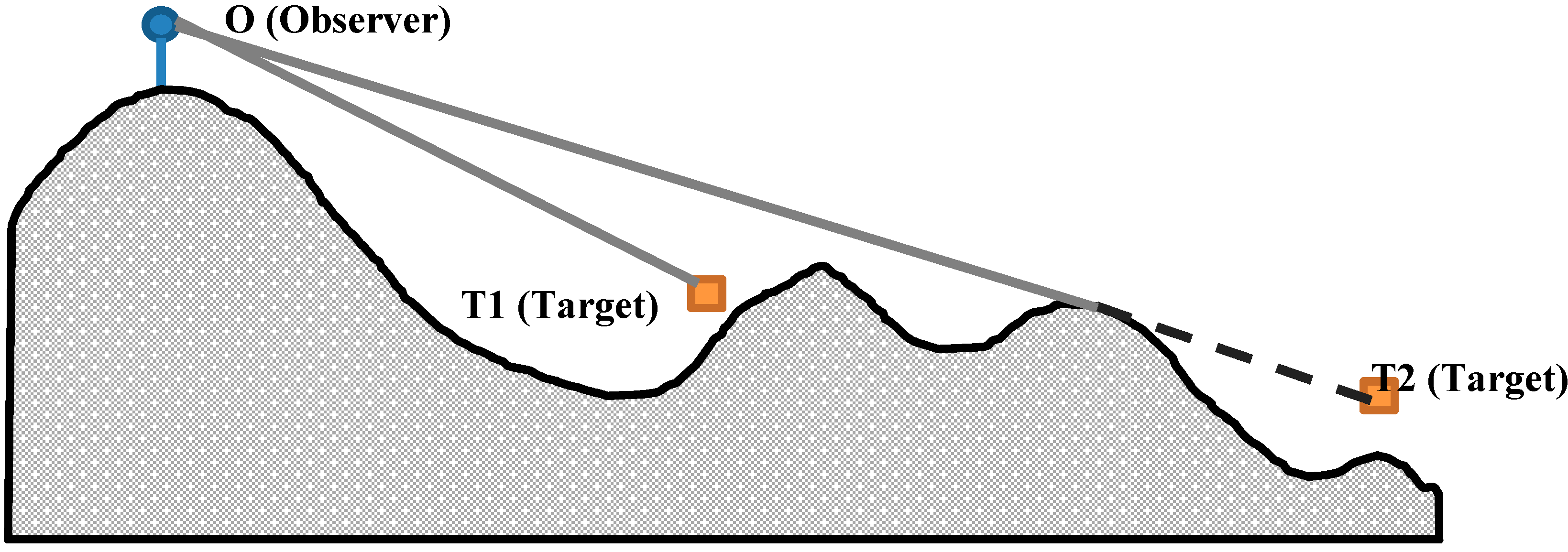In the case of camera network deployment, the line of sight may be considered as an appropriate method to model the coverage of a camera network ([19,21,27,28]). In fact, the “Line of Sight” model calculates the visibility based on a visual line from a viewpoint O (or the observer) to another point T that belongs to the target area. If this visual line intersects with any obstacle before reaching T, then T is hidden and not visible from O, otherwise, T is visible from O [27] (Figure 2).

Figure 2. Visibility based on Line of Sight. The target T1 is visible from O but the target T2 is not visible from O (Gray line: Visible, dashed line: Invisible).

Figure 2. Visibility based on Line of Sight. The target T1 is visible from O but the target T2 is not visible from O (Gray line: Visible, dashed line: Invisible).

When the visibility analysis process is applied on all points that belong to the target area, we talk about “viewshed analysis”. It results from the movement of the line of sight across the entire surface of interest [28]. The viewshed analysis can be performed based on one or many viewpoints. The result of viewshed analysis consists of determining the set of points on the surface that are visible (and that are not visible) from the set of viewpoints [27].

3.1. Construction of “Lines of Sight” for Viewshed Analysis

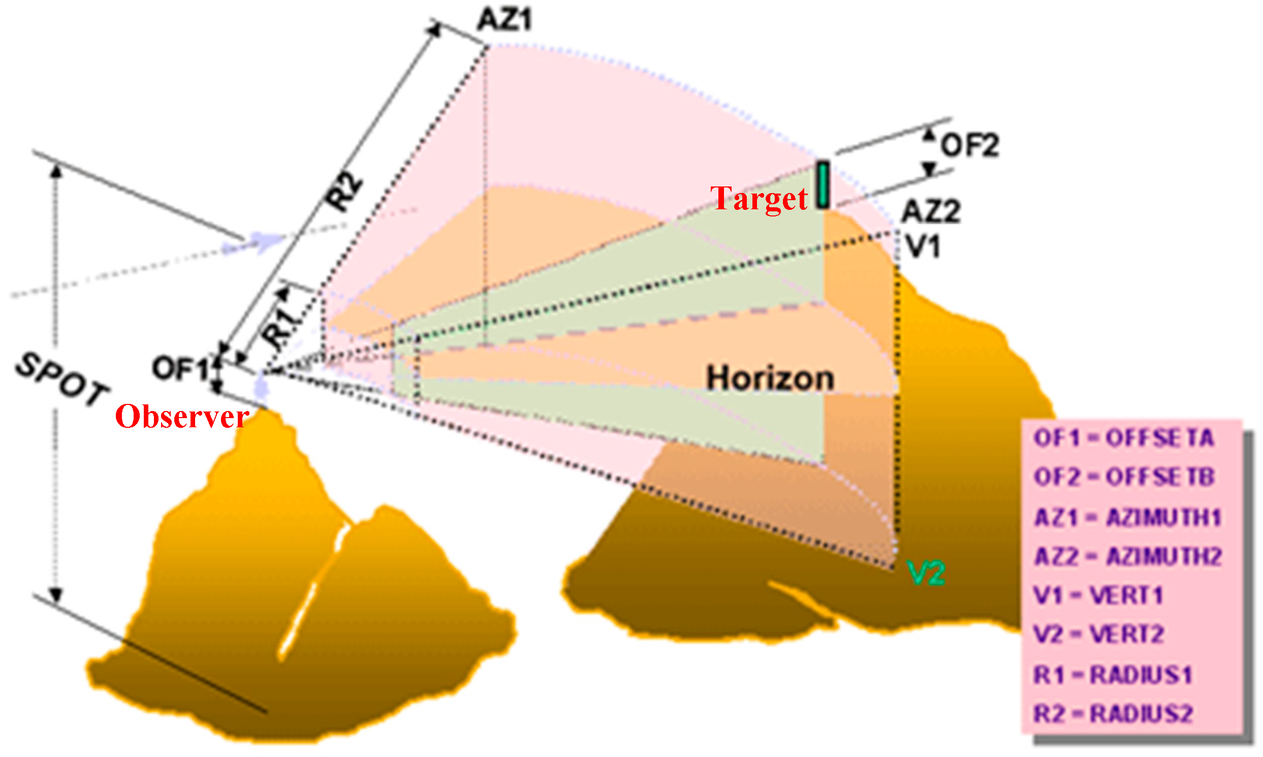
The observer point, which corresponds to the position of the camera, is characterized by its 2D coordinates (x, y) and its elevation (z). The spatial position of cameras may be determined by using a Digital Surface Model (or Digital Elevation Model) that represents the environment where the deployment will take place. In ArcGIS 10.1, which is a software designed by ESRI company, the Viewshed Analysis based on the line of sight is characterized by the following items: (1) Camera elevation value (SPOT), (2) vertical offsets (OFFSETA, OFFSETB), (3) horizontal scanning angles (AZIMUTH1, AZIMUTH2), (4) vertical scanning angles (VERT1, VERT2), and (5) scanning distances (RADIUS1, RADIUS2) (ArcGIS Help, 10.1). Figure 3 illustrates the nine parameters that are used to perform the viewshed analysis in ArcGIS 10.1.

Figure 3. The parameters used to perform viewshed analysis in ArcGIS 10.1 [29].

Figure 3. The parameters used to perform viewshed analysis in ArcGIS 10.1 [29].

Here are the explanations of the nine parameters used for controlling the viewshed analysis (ArcGIS Help, 10.1):

• SPOT: Corresponds to the ground elevation for the observer point (i.e., camera).
• OF1 and OF2: These two parameters define the vertical elevation to be added to the ground elevation of the observer OF1 (OFFSETA) and the target OF2 (OFFSETB).
• AZ1 and AZ2: These two values allow defining the range of the horizontal angle that characterizes the scan from the observer (i.e., camera). AZ1 (AZIMUTH1) corresponds to the starting angle of the scan range and AZ2 (AZIMUTH2) corresponds to the ending angle of the scan range. Note that the values of AZ1 and AZ2 may range from 0 to 360° where 0 is defined by the north direction.
• V1 and V2: These two elements delimit the vertical range of the scan from the observer. V1 (VERT1) defines the upper limit of the vertical angle and V2 (VERT2) defines the lower limit of the vertical angle. Note that V1 and V2 may vary from −90° to 90°.
• R1 and R2: These parameters determine the distance that may be covered by the observer (i.e., camera). R1 (RADIUS1) corresponds to the starting distance from which a target may be visible (the points that are closer than R1 are surely not visible). R2 (RADIUS2) corresponds to the ending distance where any point beyond this distance will be surely not visible.

3.2. Calculation of the Viewshed

Based on the nine parameters presented in the previous section, a line of sight is constructed for each point in the target area. Then, the viewshed is calculated for the environment where cameras will be placed. Let’s consider the following assumptions:

• O_i (x_i, y_i, z_i) is the observation point where “i” is the index of each observer point, i = 1, 2, …, n. Note that z_i = SPOT_i + OF1_i.
• T_j (x_j, y_j, z_j) is the target point where “j” is the index of each target, j= 1, 2, …, m. Note that z_j = H_j + OF2_i, where H_j is the elevation of the surface that corresponds to the Target T_j.
• OT_ij (x_j − x_i, y_j − y_i, z_j − z_i) is the line of sight constructed by the Observer O_i with the index “i” and the Target T_j with the index “j”. The line of sight distance is written as ||OT_ij||.

The viewshed analysis is then performed as follows; a target T_j is not visible from the Observer O_i if one of the subsequent conditions is satisfied:

(1)

The line of sight OT_ij between the Observer O_i and the Target T_j is obscured by one or many obstacles (Figure 3).

(2)

The Target T_j is outside the distance range defined by R1_i and R2_i :

(||OT_ij|| < R1_i) or (||OT_ij|| > R2_i).

(3)

The Target T_j is outside the horizontal angle range defined by AZ1_i and AZ2_i :

(Arctan((y_j − y_i)/(x_j − x_i)) < AZ1_i) and (Arctan((y_j − y_i)/(x_j − x_i)) > AZ2_i).

(4)

The Target T_j is outside the vertical angle range defined by V1_i and V2_i :

(Arcsin((z_j − z_i)/||OT_ij||) < V1_i) and (Arcsin((z_j − z_i)/||OT_ij||) > V2_i).

(5)

If all of these previous conditions (1) to (4) are not satisfied, then the Target T_j is visible from the Observer O_i.

Even if the principle of the line of sight analysis is based on a geometric approach, the implementation of the viewshed in GIS software is generally performed on a Digital Surface Model (or Digital Elevation Model) in a raster format [27]. This is due to the huge amount of calculation required to construct a line of sight for each vertex of vector data that represent a large environment. However, it is also possible to generate a viewshed analysis based on the line of sight by using a Triangular Irrigular Network (TIN) as a Digital Model for the target Area [27]. In a 3D GIS, the construction of lines of sight is based on a discrete calculation since it is necessary to specify the 3D objects from which these lines will be constructed. Similarly to vector data, the number of vertices in the 3D objects used in viewshed analysis should be reasonable in order to avoid potential software crashes when calculating all lines of sight.

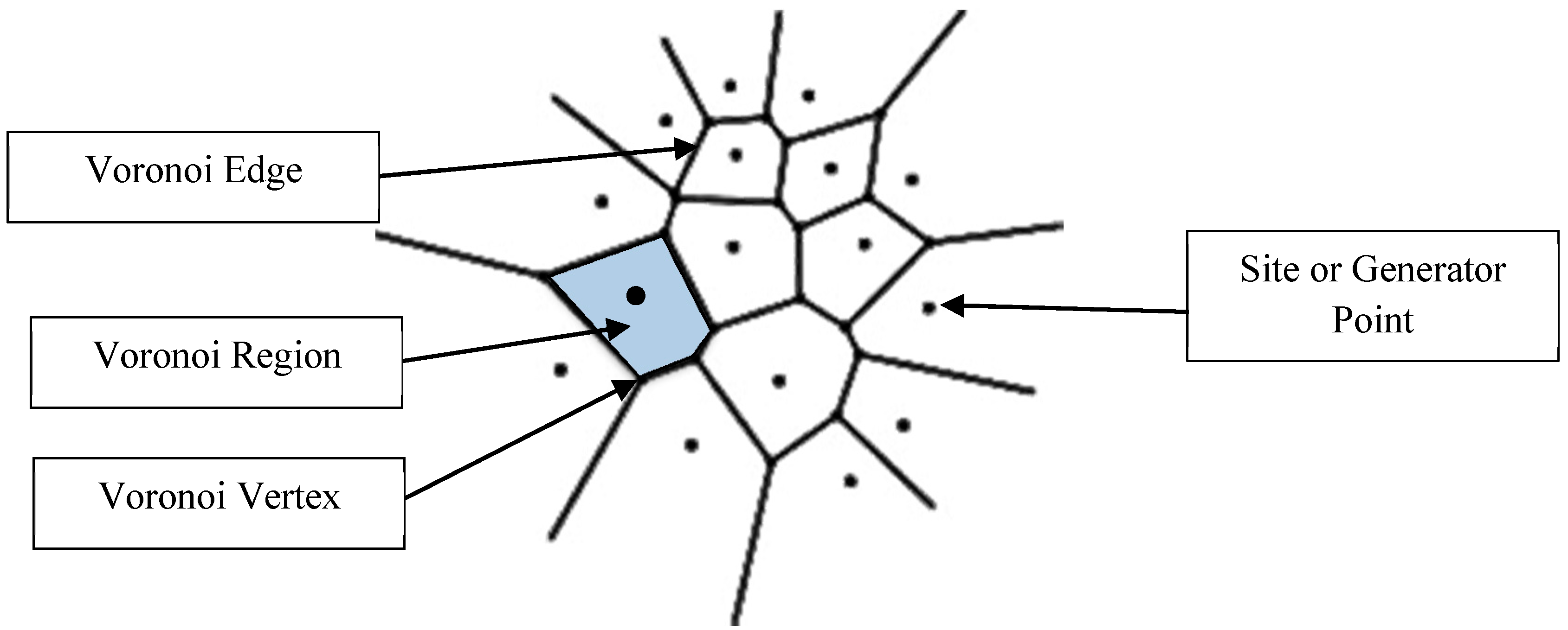
4. Basics of Voronoi Diagram

As noted in Section 2, the concept of Voronoi Diagram has been used in several studies for deploying sensor network and surveillance cameras ([19,20,21,23]). This concept is named after the mathematician Georgy Feodosevich Voronoi (1868–1908) who introduced the mathematical foundations of such a concept based on the work of Peter Gustav Lejeune Dirichlet (1805–1859) [30]. The Voronoi Diagram of a set of “sites” results from the partition (segmentation) of space into regions. Each region that corresponds to a site “s” consists of all points that are closer to “s” than any other site [31].

Formal Definition of Voronoi Diagram

Let denote S = {s₁, s₂, …, s_n} as the set of points, called “sites” or “generators”, in a space E (R² or R³). Also, consider s_i and s_j as two sites that belong to S. The dominance (DOM) of s_i over s_j may be formulated as the subset of the space E being at least as close to s_i as to s_j. This dominance may be formulated as follow [32]:

$$DOM\left(s_i,s_j\right)= \left\{ p\in E \text{|} Dist\left(p , s_i\right) \le Dist\left(p , s_j\right)\right\}$$

(1)

where: Dist (a,b) is the Euclidian Distance between point a and b and p is a point that belong to the space E.

From the foregoing, a Voronoi region (VOR) generated by a site s_i is the result of the intersection of all the dominances of s_i over the remaining sites in S. This means [32]:

$$VOR\left(s_i\right)= \underset{ s_j\in S-\left\{s_i\right\}}{{\displaystyle \mathrm{\cap }}}DOM\left(s_i,s_j\right)$$

(2)

Hence, the Voronoi Diagram (DIAVOR) generated from a set of sites S = {s₁, s₂, …, s_n} is the collection of all Voronoi regions that divides the entire space:

$$VOR\left(s_i\right)= \underset{s_j\in S-\left\{s_i\right\}}{{\displaystyle \mathrm{\cap }}}DOM\left(s_i,s_j\right)$$

(3)

Figure 4 illustrates a Voronoi Diagram that results from a set of sites:

Figure 4. A Voronoi Diagram generated from a set of “sites”.

Figure 4. A Voronoi Diagram generated from a set of “sites”.

In a Voronoi Diagram, each point on a Voronoi edge is equidistant from the two sites whose corresponding regions share this edge. Also, each vertex is equidistant from the nearest three sites that generate Voronoi regions [32]. In addition, the principles of Voronoi Diagram may be extended to different types of sites or “generators” such as lines, polygons and weighted features (point, line, polygon) instead of ordinary points [33]. Figure 5 shows Voronoi Diagrams generated from unweighted lines and polygons (A, C) and from weighted lines and polygons (B, D) that have the same shape as (A, C). The weight used in Figure 5 corresponds to the line length for B and the polygon area for D. The grayscale colors correspond to the distance (or weighted distance in case of B and D) between each point and the nearest generator feature [33]. For more details about the mathematical principles and applications of Voronoi Diagrams, the reader is referred to [30].

Figure 5. Voronoi Diagrams generated from lines and polygons. (A) Unweighted lines, (B) weighted lines, (C) unweighted polygons, and (D) weighted polygons (adapted from [33]).

Figure 5. Voronoi Diagrams generated from lines and polygons. (A) Unweighted lines, (B) weighted lines, (C) unweighted polygons, and (D) weighted polygons (adapted from [33]).

5. Camera Placement based on HybVOR Approach

The main purpose of this work is to propose a new approach for surveillance cameras deployment named “HybVOR” which belongs to the family of Landscape based methods. This approach is primarily developed for monitoring built environment. In fact, in such environment, the most important elements that should be taken into consideration in the deployment of a monitoring camera network are: Routes, building facades and entrances. It is also necessary to optimize the number of cameras while achieving the highest possible level of coverage. In our case study, which is related to the Port of Jeddah, these key elements have been confirmed by the costal guard officials (the authority responsible for protecting the security of this facility) through a questionnaire that was developed as part of this study. In addition the officials informed us that the roofs of buildings are not as important as facades or entrances. Therefore, the main objective of the HybVOR approach is to reach near 100% coverage while focusing on the following objects: (1) Routes, (2) Building facades and entrances, (3) minimum possible number of cameras.

The HybVOR approach for deploying surveillance camera network requires a Digital Elevation Model (DEM), which represents the ground elevation of the target area. In addition, it requires a 3D vector data that models buildings and their characteristics as well as other objects that can be useful for visibility calculation (such as trees and street furniture). The required data for coverage assessment comes mainly from topographic survey of the site of interest.

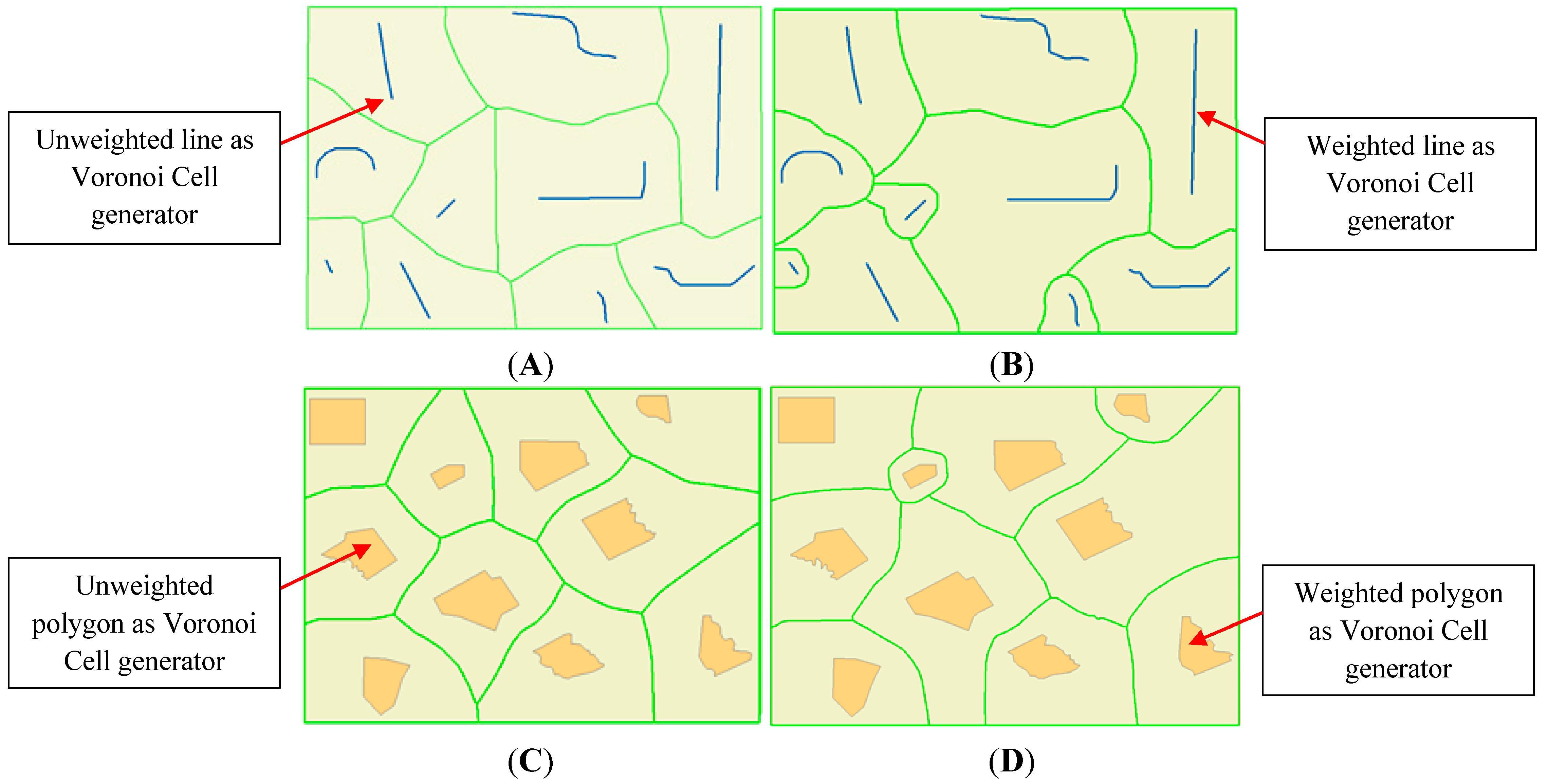
5.1. Generating Voronoi Diagram from Buildings

HybVOR approach aims to find the optimal placement of surveillance camera network based on the Voronoi Diagram generated from the footprint of buildings located in the environment. Previous Voronoi based methods that have been mentioned earlier use cameras’ positions as generator points that serve to segment the monitored space ([19,20,21,23]). Then, these methods use different algorithms to improve the level of coverage by modifying the position of cameras or adding new ones. All of these methods do not provide an effective way to define an initial position of cameras that is as close as possible to the optimal placement. The HybVOR approach provides an original method to overcome this weakness. The principle is to use buildings as generator objects for the Voronoi Diagram. Thereafter, surveillance cameras will be placed on Voronoi edges. This kind of placement allows achieving three main objectives: (1) Minimizing the number of cameras for maximum possible coverage, (2) Providing better observability for buildings facades and entrances, and (3) Ensuring maximum coverage for roads.

5.1.1. Minimizing the Number of Cameras for a Maximum Possible Coverage

It is known that the points belonging to a Voronoi edge have the property of being equidistant to generator objects that share this edge. Thereby, if a camera is placed on a Voronoi edge, it will be as close as possible to the two corresponding buildings (which are the generator objects) at the same time. In addition, if a camera is placed much closer to a building, it will be automatically farther from the facing building. This could increase the required number of cameras in order to cover the whole environment. 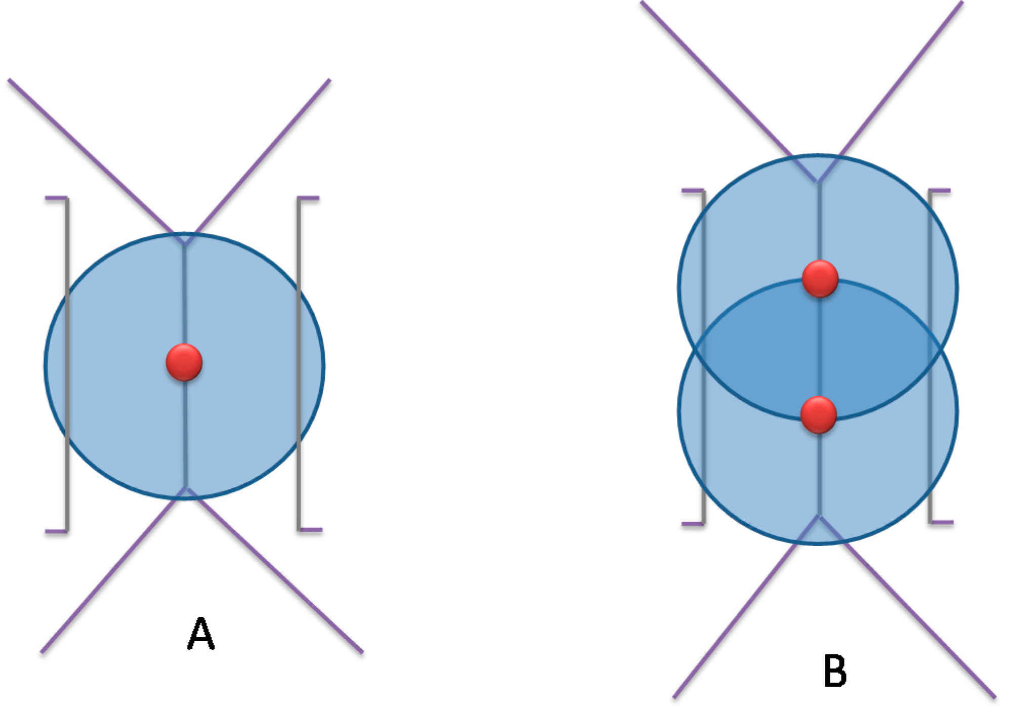Figure 6 illustrates the advantage of placing cameras on Voronoi edge in order to reduce their number. Note that the total number of cameras required to cover an entire area depends on the parameters of the cameras to be installed. Section 5.2 is dedicated to explain the methodology used for deploying cameras on Voronoi edges depending on the parameters of cameras and the location of buildings.

Figure 6. Advantage of placing camera on a Voronoi edge. (A) Camera is placed on the Voronoi edge, (B,C) Camera is placed farther from the Voronoi edge.

Figure 6. Advantage of placing camera on a Voronoi edge. (A) Camera is placed on the Voronoi edge, (B,C) Camera is placed farther from the Voronoi edge.

5.1.2. Providing a Better Observability for Buildings Facades and Entrances

In order to have a better observability, objects in the environment have to be as a large as possible in the image or the video [6]. To achieve this goal, it is necessary to minimize the “Foreshortening effect”. This effect impacts the quantity of information that may be extracted from an observation [1]. The foreshortening effect appears when the angle between the camera’s view and the object becomes increasingly smaller. Accordingly, the projection of the object on the camera’s image plan will decrease and the monitored object will appear shorter on the image [6]. 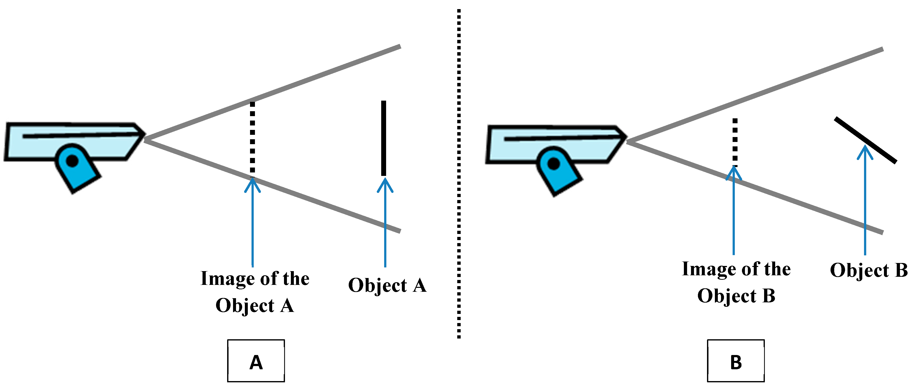Figure 7 highlights the impact of the foreshortening effect.

Figure 7. The impact of the foreshortening effect. (A) Image without foreshortening effect and (B) image with foreshortening effect.

Figure 7. The impact of the foreshortening effect. (A) Image without foreshortening effect and (B) image with foreshortening effect.

In the case of monitoring a built environment, and taking into consideration the possible minimum number of cameras, the placement of a camera closer to a building than the facing one will increase the foreshortening effect when the camera is directed to the farthest building. The appearance of the shortening effect may be caused by the large distance of the farthest building compared to the nearest one, especially if the angle between the camera’s view and the facade of the farthest building to be monitored is small. Therefore, deploying cameras on Voronoi edges will optimize foreshortening effects in both sides, and hence, provide better observability for building facades and entrances.

5.1.3. Ensuring a Maximum Coverage for Roads

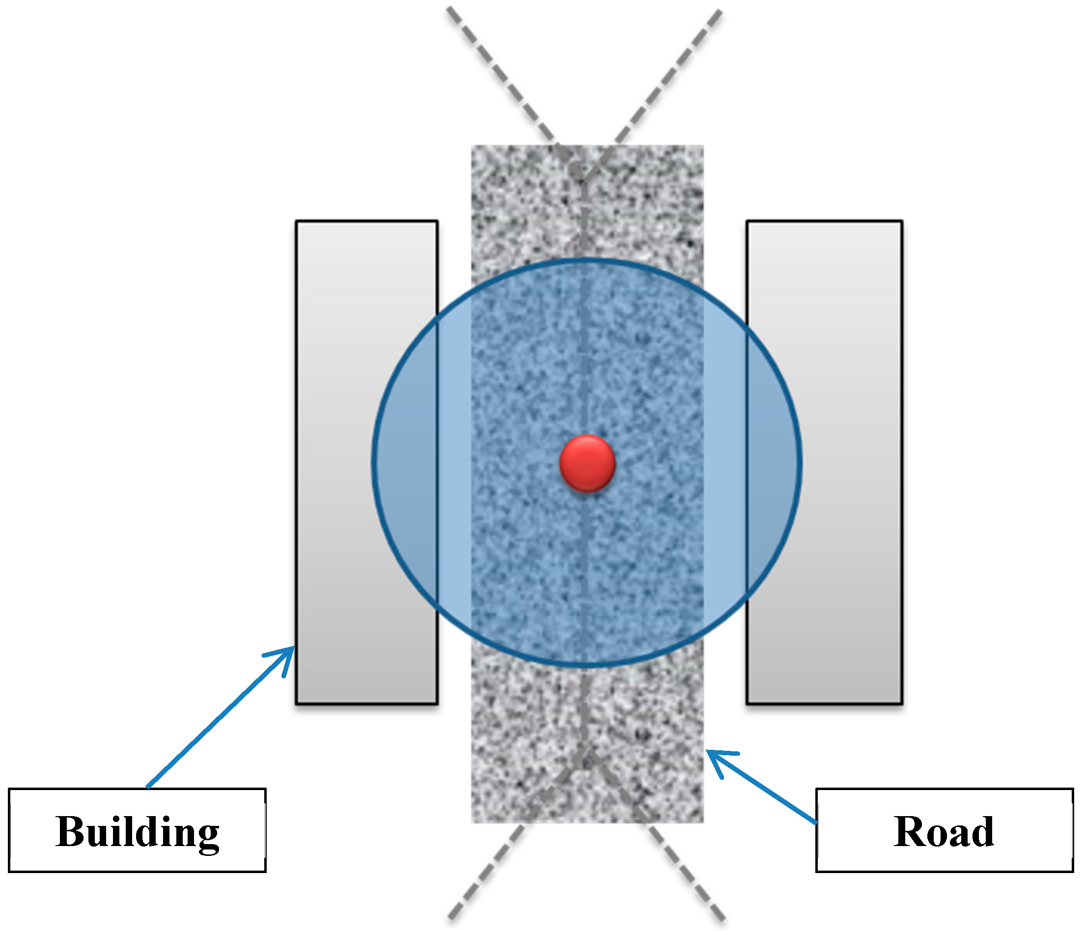
In general, roads are constructed to ensure access to the buildings within a built environment. Therefore, roads are almost located at equal distance from buildings they serve. Hence, the Voronoi edges generated from footprints of buildings will be quite close to roads that are built in the environment. Thereby, the placement of cameras on Voronoi edges will provide a better observability and coverage for roads while minimizing the number of cameras (Figure 8).

Figure 8. Camera placement on the Voronoi edge for a better observability and coverage for roads.

Figure 8. Camera placement on the Voronoi edge for a better observability and coverage for roads.

5.2. Deploying Camera Network

After highlighting the importance of placing cameras on Voronoi edges in Section 5.1, the next step is to find the best position of each camera in order to achieve the maximum possible coverage while minimizing the number of cameras. To do so, the best location on the Voronoi edge will be defined based on three constraints: (1) Parameters of cameras, (2) the location of buildings and (3) minimizing the foreshortening effect.

In this work, two assumptions are considered; the first one is that cameras should be installed on poles. This statement has been confirmed by the costal guard of Jeddah Seaport. The second assumption states that all cameras have the same following parameters (c.f. Section 3.1):

-

OFFSETB = 0 (there is no artificial target on the field).

-

AZIMUTH1 = 0° (the starting horizontal angle).

-

AZIMUTH2 = 360° (the ending horizontal angle of the scan range).

-

VERT1 = 90° (the upper limit of the vertical angle).

-

VERT2 = −90° (the lower limit of the vertical angle).

-

RADIUS1 = 0 (the starting distance from which a point may be visible).

-

RADIUS2 = Constant (the ending distance where any point beyond this distance will be surely not visible, this parameter represent the camera range).

There are two other parameters of cameras that may take varying values, which are SPOT and OFFSETA:

-

SPOT corresponds to the ground elevation where the camera will be placed.

-

OFFSETA is related to the height of buildings to be monitored from each camera.

In order to generate Voronoi diagrams, buildings’ footprints are used as generator objects. These footprints may be produced either from an existing model of 3D buildings or form topographic surveys. Once the Voronoi diagram is generated, each edge will be split from one of its two Voronoi vertices based on the camera range as follows:

• If the length of a Voronoi edge is less than the range of the camera, then this edge will not be divided.
• If the length of a Voronoi edge is more than the range of the camera, then this edge will be divided into equal segments. The number of these new segments is calculated based on the following procedure:

$$IF ((L_{VE })Mod \left(R_{Cam }\right)=0) Then Ns=Ceil \left(\frac{L_{VE}}{R_{Cam}}\right)$$

(4)

$$\text{ELSE }(({\text{L}}_{\text{VE }})\text{Mod }\left({\text{R}}_{\text{Cam }}\right)<>0)\text{ Then Ns}=\text{Ceil }\left(\frac{{\text{L}}_{\text{VE}}}{{\text{R}}_{\text{Cam}}}\right)+1$$

(5)

where:

-

Ns: is the number of new segments generated from splitting a Voronoi Edge.

-

Ceil: is the mathematical function that calculates the integer part of a number (for example Ceil(1.45) = 1).

-

Mod: is the mathematical function that calculates the remainder of a division.

-

L_VE: is the original length of the Voronoi edge.

-

R_Cam: is the range of the camera.

Thereafter, the length of each new generated segments will be equal to:

$$L_{SpVE }=\left(\frac{L_{VE}}{Ns}\right)$$

(6)

where L_SpVE is the length of each new segment that is produced form splitting the corresponding original Voronoi edge.

Figure 9. Placing Cameras on Voronoi edge. (A) Voronoi edge length is less than camera range, (B) Voronoi edge length is more than camera range.

Figure 9. Placing Cameras on Voronoi edge. (A) Voronoi edge length is less than camera range, (B) Voronoi edge length is more than camera range.

Following the subdivision of a Voronoi edge into equal segments, a camera is placed at the midpoint of each new segment. The choice of placing cameras in such a way increases the observability of buildings. Indeed, if a camera is placed on a Voronoi Vertex, it may cause narrow angles to monitor buildings (and building entrances in particular), which is one of the main reasons behind the foreshortening problem. Figure 9 shows the placement of cameras in the middle of Voronoi segments with respect to the surrounding buildings (c.f. Section 5.1).

The choice of dividing Voronoi edges based on the camera range comes from the idea that each camera should be visible by the two adjacent cameras (front and rear). Hence, the distance between two successive cameras will always be less than the camera range. Therefore, if a camera fails, there will be no surveillance hole (or non-covered region) along the Voronoi edge, which makes the coverage still acceptable until repairing the broken camera. Figure 10 illustrates the coverage area due to the failure of a camera.

Figure 10. The coverage area after the failure of one camera.

Figure 10. The coverage area after the failure of one camera.

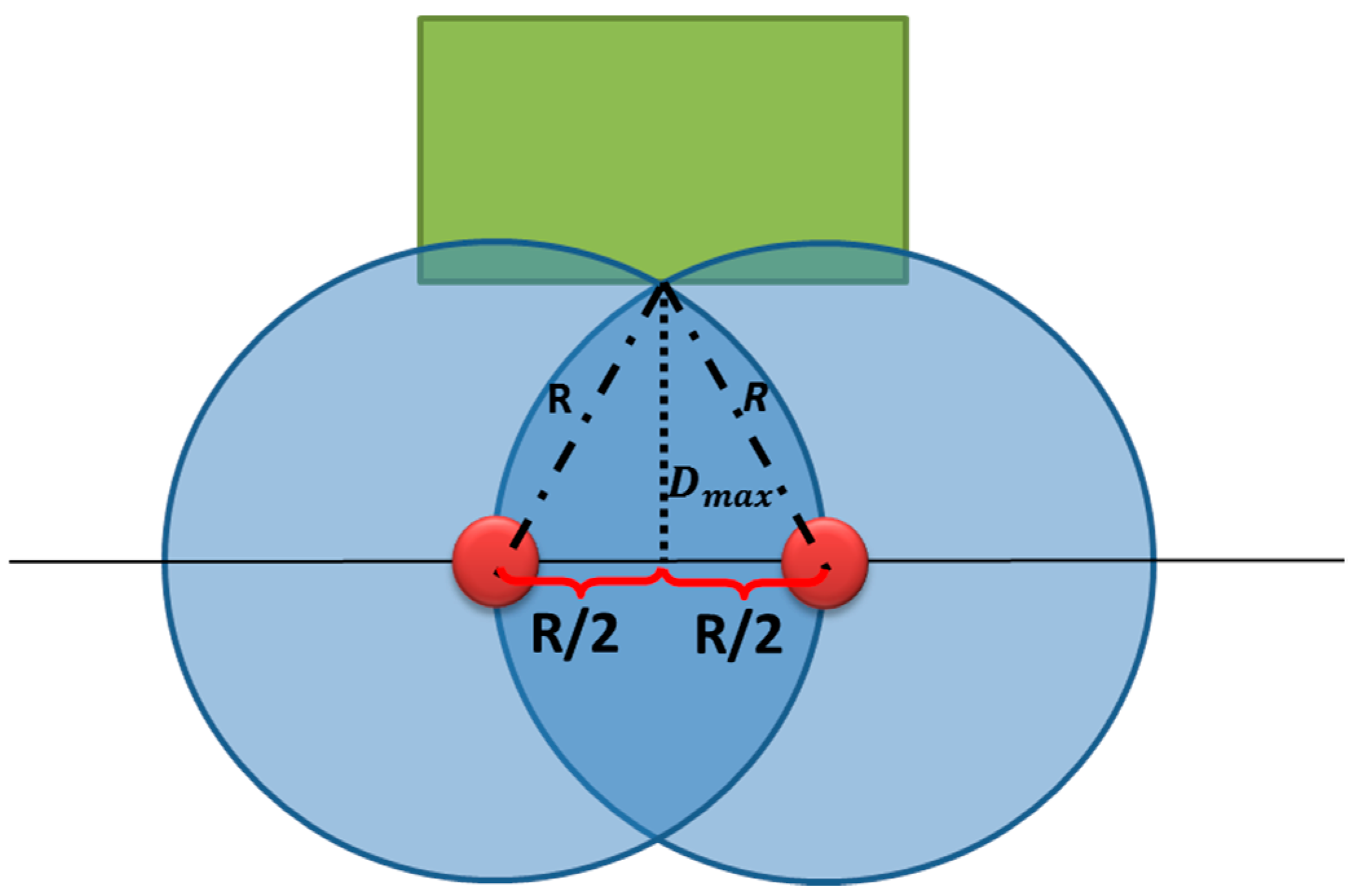
In order to ensure an efficient surveillance, cameras must be placed at a distance that allows full observability of facades and entrances of buildings (Buildings’ roofs have a lower priority in our case study according to the confirmation of the coastal guard). Therefore, it is necessary to determine the maximum allowed distance among buildings and Voronoi edges to ensure a maximum coverage of facades and entrances. Figure 11 shows the method used for calculating this distance depending on the camera range and the distance between two adjacent cameras (this distance should not exceed the camera range).

Figure 11. The maximum allowed distance D_max among buildings and the Voronoi edge.

Figure 11. The maximum allowed distance D_max among buildings and the Voronoi edge.

where, R is the range of cameras and D_max is the maximum allowed distance between a building and a Voronoi edge. Based on Figure 11, the distance D_max is equal to:

$$D_{max}=\left(\sqrt{3}/2\right)\times R$$

(7)

It is important to note that D_max in Equation (7) is an approximation according to a 2D assumption. Its calculation based on a 3D assumption will give values that are almost equal for cameras that have a height of about 10m.

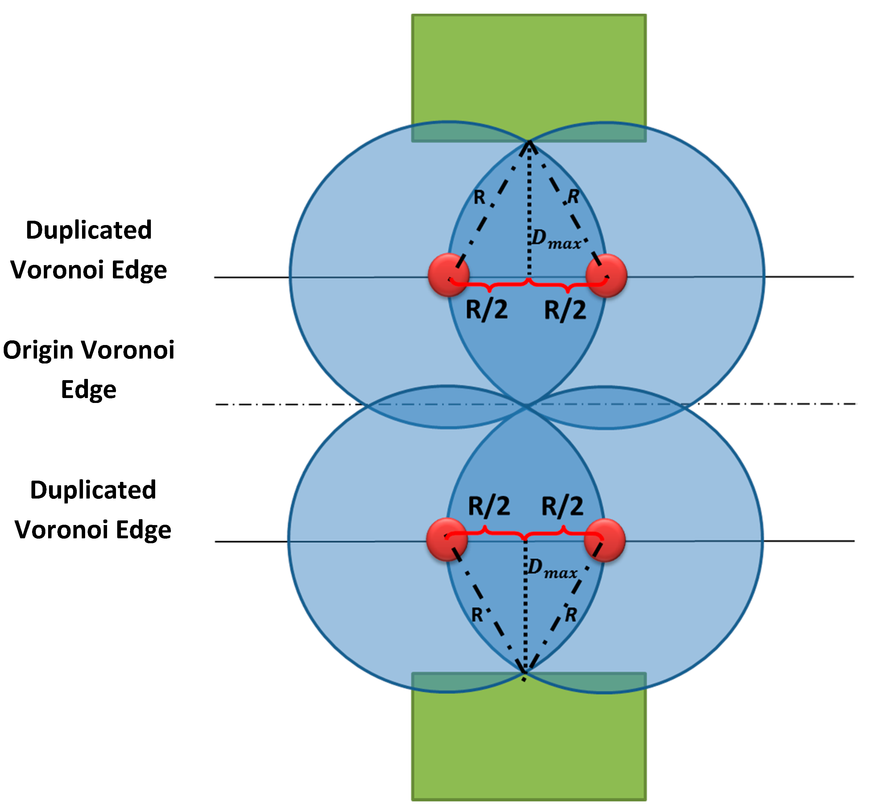
In the case where one of buildings is far from the Voronoi edge with a distance greater than the maximum distance mentioned earlier, a duplication of this Voronoi edge is required (Figure 12). The deployed cameras on this duplication edges have to meet the following two conditions:

• The distance between a duplicated Voronoi edge and the corresponding building should not be further than the distance D_max mentioned in Equation (7).
• Cameras placed on a duplicated Voronoi edge should ensure a full coverage of the origin Voronoi edge.

Note that if a building is far from the Voronoi edge with a given distance, the facing building will also be far from the shared Voronoi edge with almost the same distance.

Figure 12. Duplication of the Voronoi edge and the corresponding number of cameras.

Figure 12. Duplication of the Voronoi edge and the corresponding number of cameras.

At this stage, the location of the camera network is obtained based on the Voronoi Diagram generated from the footprint of buildings. In Section 5.3, these cameras’ positions are used to assess and calculate the level of coverage through a hybrid approach that combines raster and 3D Vector analysis of visibility.

5.3. Hybrid Assessing of the Camera Network Coverage

After defining the location of cameras, the level of coverage is assessed based on viewshed calculation. The proposed HybVOR approach consists of combining two methods for viewshed calculation: Raster-based and 3D Vector-based.

5.3.1. Raster-Based Viewshed Calculation

This method allows assessing the degree of coverage of an area of interest based on a Digital Surface Model (DSM) in raster format. This DSM results from the combination of the ground elevation with buildings’ height. In order to create such a DSM, a Digital Elevation Model (DEM) in raster format that represents the ground elevation has to be generated. The raster DEM is generally extracted from a Triangular Irregular Network (TIN) that represents the elevation of the ground. Then, buildings’ footprints are generated either from an existing 3D Model of buildings or from topographic surveys. After that, these footprints that are in vector format are converted to a raster format using the same resolution of the original DEM. The pixel values in this resulting raster correspond to the roof elevation of each building. Thereafter, the raster file that represents the elevation of buildings’ roofs is combined with the raster DEM that corresponds to the ground elevation. Here are the main steps to perform this combination:

-

For each pixel that belongs to the resulting DSM:

• If the corresponding value in the building’ roof raster file is null then the pixel value is taken from the raster DEM.
• Otherwise, the pixel value is taken from the corresponding pixel in the building’ roof raster file.

The combination of the Raster DEM and the elevation information from 3D Buildings Model will provide a Digital Surface Model in raster format for the area of interest. This DSM is mandatory in order to assess the coverage of camera network through the HybVOR approach.

After generating the DSM, each camera should have a height value, which corresponds to OFFSETA (c.f. Section 3.1). This offset value will be chosen according to the height of the two buildings which are considered as generators of the Voronoi edge where the camera is placed. The camera height is mainly related to the possibility of constructing poles to place cameras. Two situations occur:

The first case happens when the surrounding buildings of the camera pole are not very tall. In this situation, the value of the camera height will correspond to the tallest building. The advantage of this criterion is offering the possibility of monitoring the roofs in addition to entrances and facades. Otherwise, if it is not feasible (or not profitable) to construct a pole that has the same height as the taller building, a standard height for the pole to place the camera has to be chosen. However, the roof of buildings may be not visible from the camera. This will not have a great impact in our case because buildings’ roofs do not have a high importance as mentioned Section 5.2.

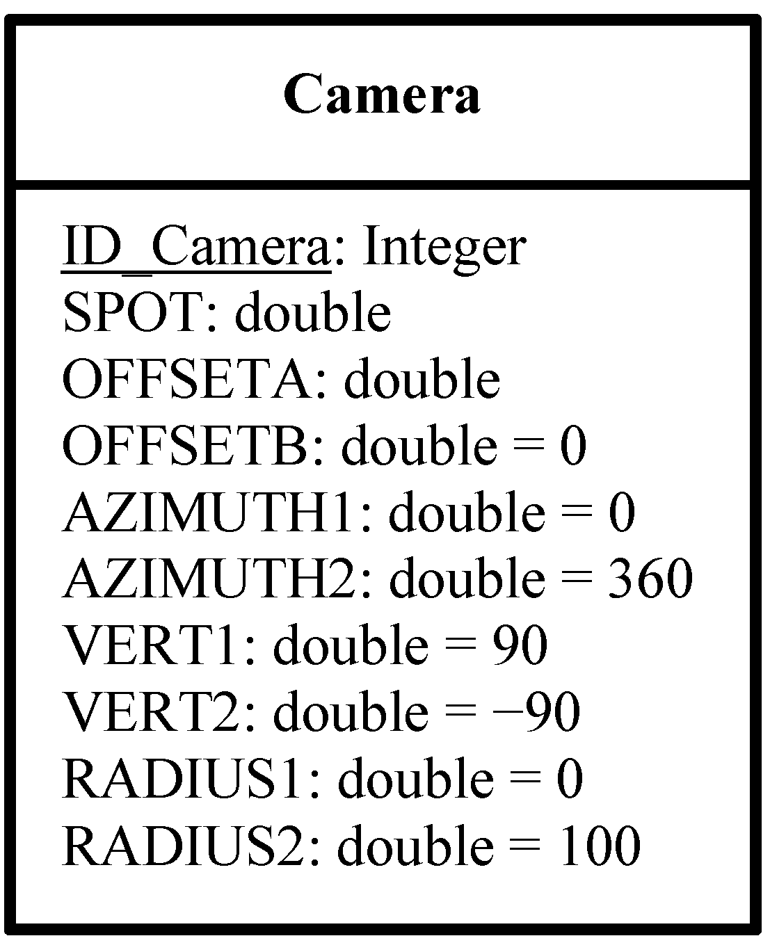
The main parameters of cameras to be deployed (which are explained in Section 3.1 and Figure 3) will be integrated in the attribute table of the point feature class representing the 2D placement of the camera network. Figure 13 shows the attribute table of the class “Camera”. In this example, the range of all cameras is constant and equal to 100 m. As mentioned previously, the parameters OFFSETB, AZIMUTH1, AZIMUTH2, VERT1, VERT2, RADIUS1 and RADIUS2 are also constant. However, SPOT and OFFSETA may vary depending on the location of each camera. The attribute ID_ Camera represents the primary key of the class “Camera”, i.e., that each camera will have a unique identifier.

Figure 13. The attribute table of the class “Camera”.

Figure 13. The attribute table of the class “Camera”.

Once the raster DSM (which combines the ground elevation with the Building height) and the feature class that represents cameras (with their location and attribute) have been generated, the viewshed is calculated. The idea is to apply the methodology presented in Section 3.2 to assess each pixel if it is visible or not from one or more cameras belonging to the deployed network. The attribute table of the class “Camera” is used to provide the parameters of cameras that were required to calculate the Viewshed. In Section 6.2, the results of the raster Viewshed calculation based on a DSM that represents an area of Jeddah Seaport are presented.

5.3.2. 3D Vector-Based Analysis of Visibility

The benefit of using a 3D vector model is to perform visibility analysis on elements that cannot be assessed based on a raster DSM. Indeed, a raster DSM allows only the Viewshed calculation of objects and features that are on the surface. Hence, roofs are the only components of buildings that may be present in a raster DSM. Other vertical components of buildings such as facades, doors, windows cannot be modeled in a raster DSM. For this reason, it is necessary to complete the coverage assessment of the camera network with a 3D vector-based analysis of visibility. 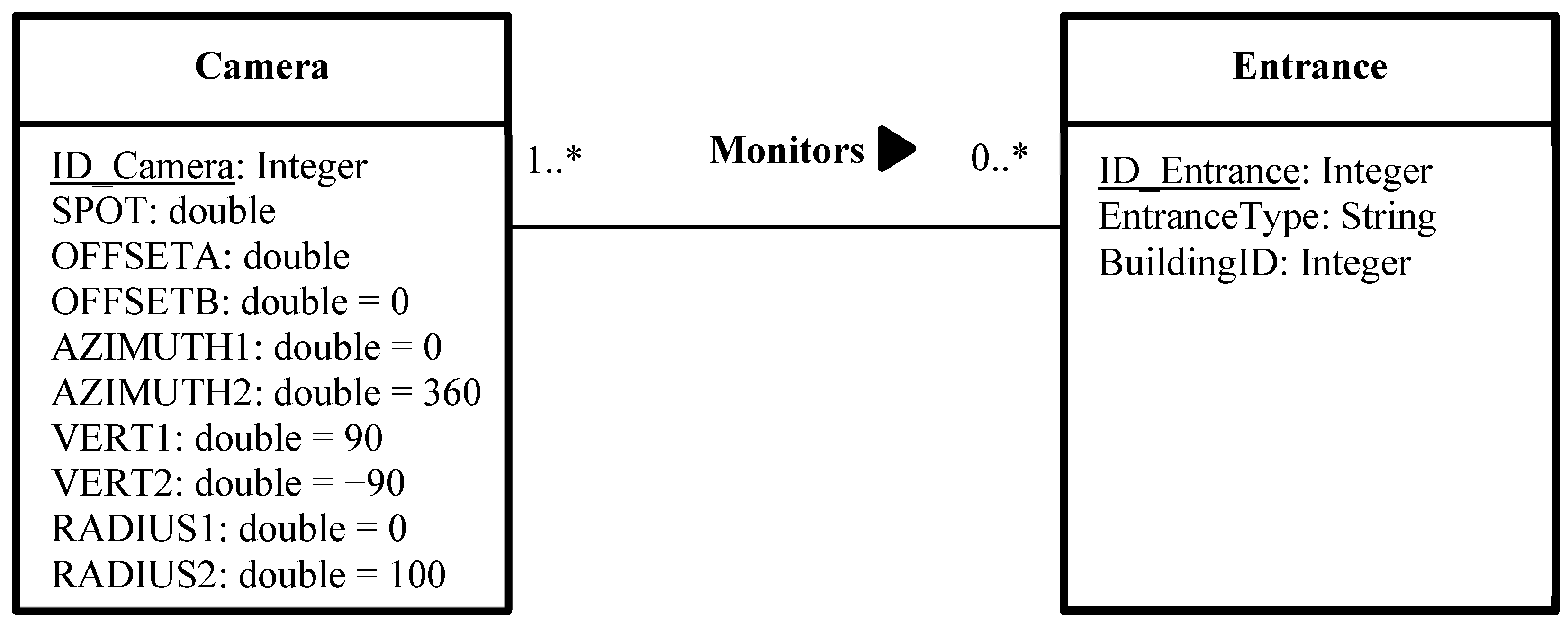This method of visibility analysis consists of constructing lines of sight among each camera and objects of interest that will be monitored from this location (Figure 2). To do so, it is necessary to establish a many-to-many relationship between the class “Camera” and the class that represents the objects to be monitored. The class “Camera” contains very important information about the properties and the 3D position of cameras, which are necessary to configure the spatial layout of the deployed network. In our case, the class “Entrance” represents the main entrances of buildings (doors and windows). This many-to-many relationship means that a camera may monitor zero, one or many entrances, and an entrance has to be monitored by one or many cameras (Figure 14). In the absence of such a relation, the software will create a line of sight between each camera and all vertices in the 3D model, which will lead to an excessive amount of time and provides results which are difficult to interpret. Figure 14 shows the UML notation of the many-to-many relationship between the classes “Camera” and “Entrance”.

Figure 14. Unified Modeling Language notation of the many-to-many relationship between the classes “Camera” and “Entrance”.

Figure 14. Unified Modeling Language notation of the many-to-many relationship between the classes “Camera” and “Entrance”.

The constructed lines of sight represent straight lines that link between the observation point (camera) and the target feature. It is possible to construct several lines of sight between a camera and a target feature if this latter is either a line or polygon feature by applying a sampling distance.

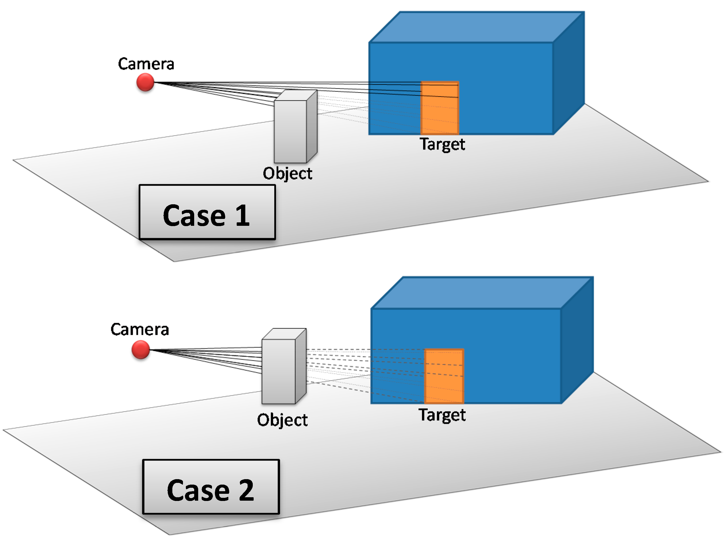
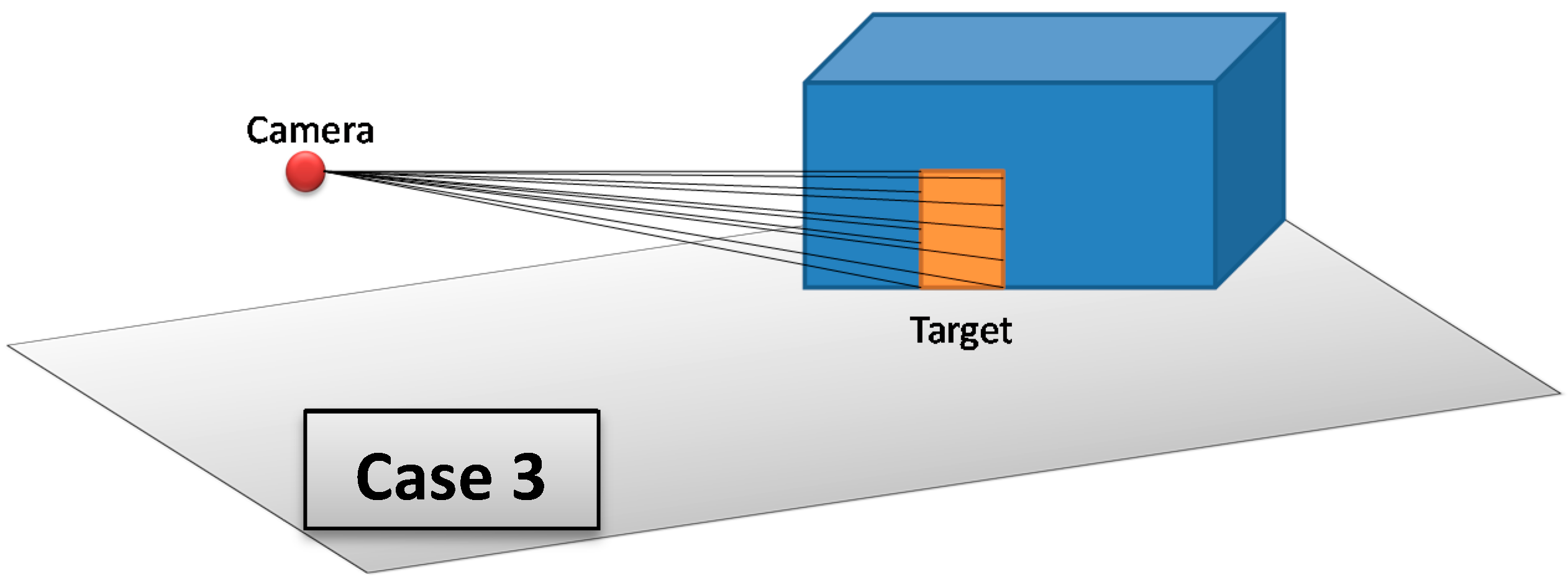
The 3D Vector-based analysis of visibility consists of combining 3D models that represent objects in the monitored environment with the constructed lines of sight. The aim is to check whether these objects intersect the lines of sight between the camera and the target. Three cases may occur (Figure 15):

• If there are one or many objects in the environment that intersect all lines of sight between the camera and the target, then this target is completely invisible from the camera.
• If there are one or many objects in the environment that intersect some lines of sight (not all lines of sight) between the camera and the target, then this target is partially visible from the camera.
• If there is no object that intersects lines of sight between the camera and the target, then this target is fully visible form the camera.

Figure 15. Three possible cases that may result from 3D Vector-based analysis of visibility; Case 1: The target is partially visible, Case 2: The target is completely not visible, and Case 3: The target is fully visible.

Figure 15. Three possible cases that may result from 3D Vector-based analysis of visibility; Case 1: The target is partially visible, Case 2: The target is completely not visible, and Case 3: The target is fully visible.

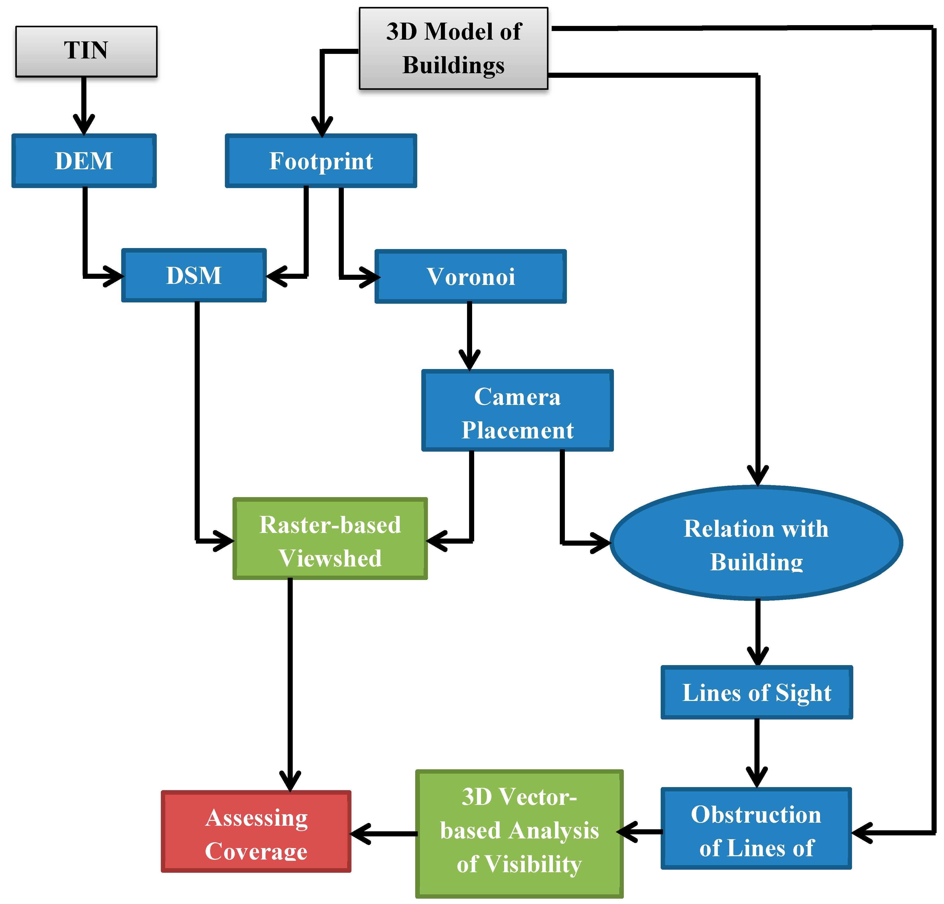
Figure 16 summarizes the main steps in the implementation process of the HybVOR approach for deploying surveillance camera network.

Figure 16. The main phases of implementing the Hybrid Voronoi (HybVOR) approach.

Figure 16. The main phases of implementing the Hybrid Voronoi (HybVOR) approach.

In Section 6, the results of implementing the HybVOR approach are presented. The aim is to find the optimal placement of camera network for monitoring an area of interest in Jeddah Seaport.

6. Results and Discussion

In this section, the case study that corresponds to Jeddah Seaport located in the kingdom of Saudi Arabia is introduced. This case study has been chosen because the border guard of Jeddah Seaport has stressed that the current deployed video surveillance camera system is not fully efficient due to two main reasons. First of all, the placement of cameras in its current state does not meet their expectations because there are some areas of the seaport that are overloaded by many cameras, while other places are not well covered. Secondly, the current total coverage of Jeddah Seaport is around 50%, while the border guard aims to achieve a coverage close to 100% with an optimal number of cameras.

In the following, the adopted methodology for acquiring data that are necessary to implement the HybVOR approach is presented. Then, the results obtained by deploying surveillance camera network based on our proposed approach are highlighted. Afterward, the results of the HybVOR implementation are discussed.

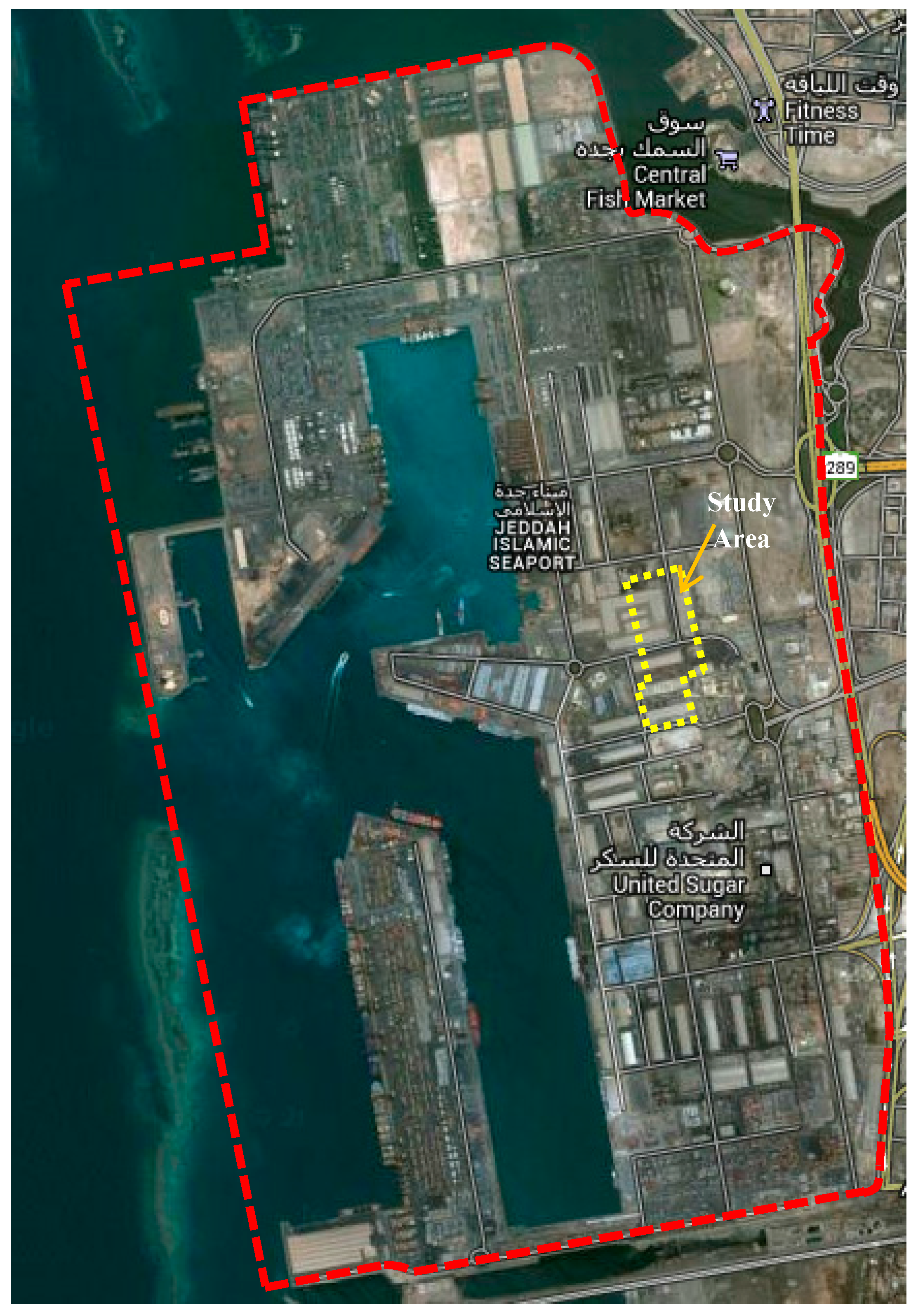
6.1. Case Study: Jeddah Sea Port

Jeddah Seaport is the most important seaport in the Kingdom of Saudi Arabia. It has a strategic location in the middle of the Red Sea, it is located at 21°28ʹ North Latitude and 39°10ʹ West Longitude. Jeddah Seaport serves the two Muslim Holy cities Mecca and Medina in the Kingdom of Saudi Arabia (Jeddah Seaport, 2013). It occupies 10.5 square kilometers, with 58 deep water quays having an overall length of 11.2 kilometers with a draft reaching 16 meters [34]. Figure 17 shows a general overview of Jeddah Seaport and our study area.

In order to prepare the required data for implementing the HybVOR approach, namely: (1) a Digital Elevation Model (DEM), (2) a Digital Surface Model (DSM) and (3) a 3D Model of Buildings, topographical surveys (based on a combination of GPS, Total Station and Level) were undertaken to acquire spatial data with the required accuracy for large scale plans (1:500).

The first phase consists of exploring the area of interest and conducting a preliminary study of pertinent data to be acquired. Thereafter, 20 Ground Control Points (GCPs) were defined with a horizontal accuracy of 5 cm and a vertical accuracy of 3 cm. In order to determine the planimetric position of these GCPs, a differential GPS survey in rapid static mode for 10 GCPs was conducted. For the other 10 GCPs, a traversing method with total station was adopted because of the poor quality of GPS signal. In terms of GCPs elevation, a direct levelling method was used to measure differences in elevation. Then, the absolute values of elevations were calculated based on a reference point which has a known elevation in our study area.

Once the horizontal and vertical coordinates of GCPs are determined, a detailed topographic survey of elements in the study area is carried out. These elements are relevant for performing the deployment of surveillance cameras according to the HybVOR approach. To acquire 3D details of buildings, a reflectorless total station was used (with a range of 500 m and a precision of 3 mm + 2 ppm). This type of total station facilitates acquiring details that are hardly or not accessible in the environment. Regarding the acquisition of elevation data related to terrain and streets, the indirect leveling method with total station was used. A regular grid of 5 m for ground elevation data is adopted because the terrain was quite homogenous.

The elevation data corresponding to the ground were used for generating a Triangular Irregular Network (TIN) which will serve to create a raster DEM. 3D details of buildings are the basis for creating a 3D model of the study area. Such a 3D model has a major role in the HybVOR approach in terms of generating Voronoï diagram, producing DSM, performing raster based viewshed, and carrying out 3D Vector-based analysis of visibility.

Figure 17. General overview of Jeddah Seaport and the study area (image from Google Maps).

Figure 17. General overview of Jeddah Seaport and the study area (image from Google Maps).

6.2. Results

Based on topographical surveys, a set of terrain elevation points and a 3D detailed survey of routes and buildings have been acquired. Then, this data is exported to ArcGIS in order to implement our HybVOR approach for the placement of the camera network and performing the analysis of the expected level of coverage.

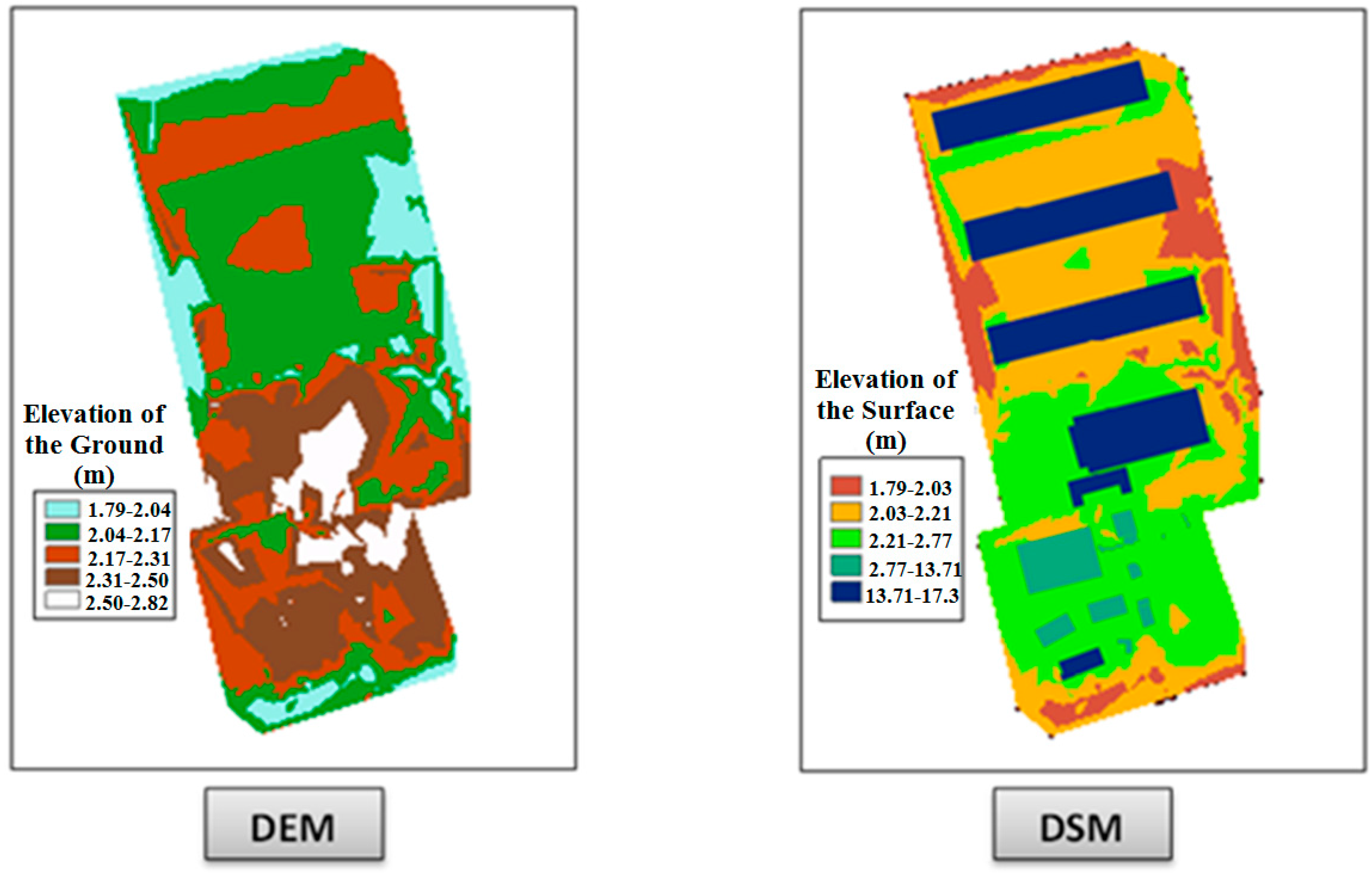
For this purpose, the first step is to generate a Raster Digital Elevation Model (DEM) from the set of terrain elevation points structured in a Triangular Irregular Network (TIN). Then, the buildings’ footprints are produced from the 3D detail survey and assigned a value of elevation to each footprint based on the elevation of the corresponding building. Thereafter, these footprints are transformed to raster format, and they are combined with the DEM in order to generate a Raster Digital Surface Model (DSM) of the region of interest. This DSM is the basis of our raster based viewshed calculation (c.f. Section 5.3). Figure 18 shows the DEM and the DSM that were used in our raster based viewshed calculation.

Figure 18. The Digital Elevation Model (DEM) and Digital Surface Model (DSM) used for raster based viewshed calculation.

Figure 18. The Digital Elevation Model (DEM) and Digital Surface Model (DSM) used for raster based viewshed calculation.

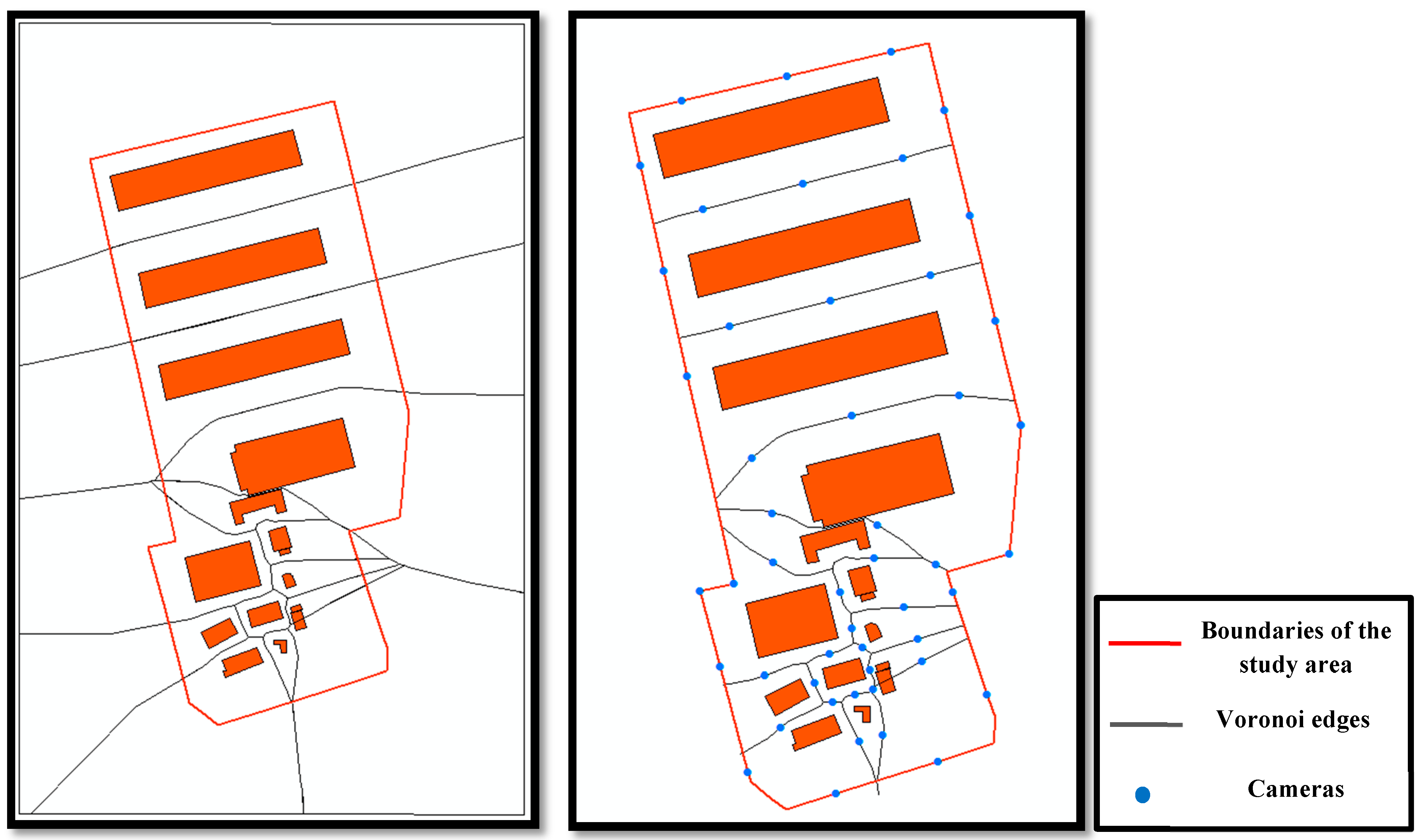
The second step consists of generating the Voronoï diagram (in vector format) based on buildings’ footprint. Then, a camera network is placed according to HybVOR approach on the divided Voronoï edges as explained in Section 5.2. Figure 19 illustrates the placement of the camera network in our study area based on HybVOR approach. It is important to notice that, in theory, the Voronoï edges generated from polygons should appear as parabola curves. However, due to the drawing limitation of the used GIS software, the parabola curves are approximated to line segments, and this approximation will not affect the quality of coverage assessment [35].

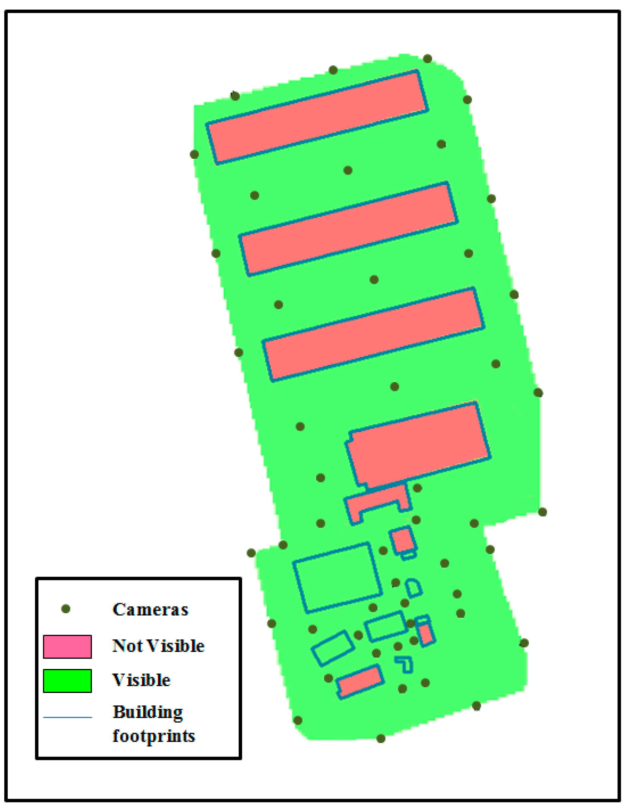
In the third phase, the viewshed is calculated based on the generated raster DSM and cameras’ position. The main purpose of this phase is to ensure that the road network is fully covered by the surveillance camera network. Regarding the elevation of cameras, it corresponds the tallest building to be monitored from this location (c.f. Section 5.3). Figure 20 shows the level of surface coverage obtained by applying the HybVOR approach in the region of interest.

Figure 19. Camera network deployment on the study area based on HybVOR approach.

Figure 19. Camera network deployment on the study area based on HybVOR approach.

Figure 20. Surface coverage generated from the DSM and the proposed cameras’ location.

Figure 20. Surface coverage generated from the DSM and the proposed cameras’ location.

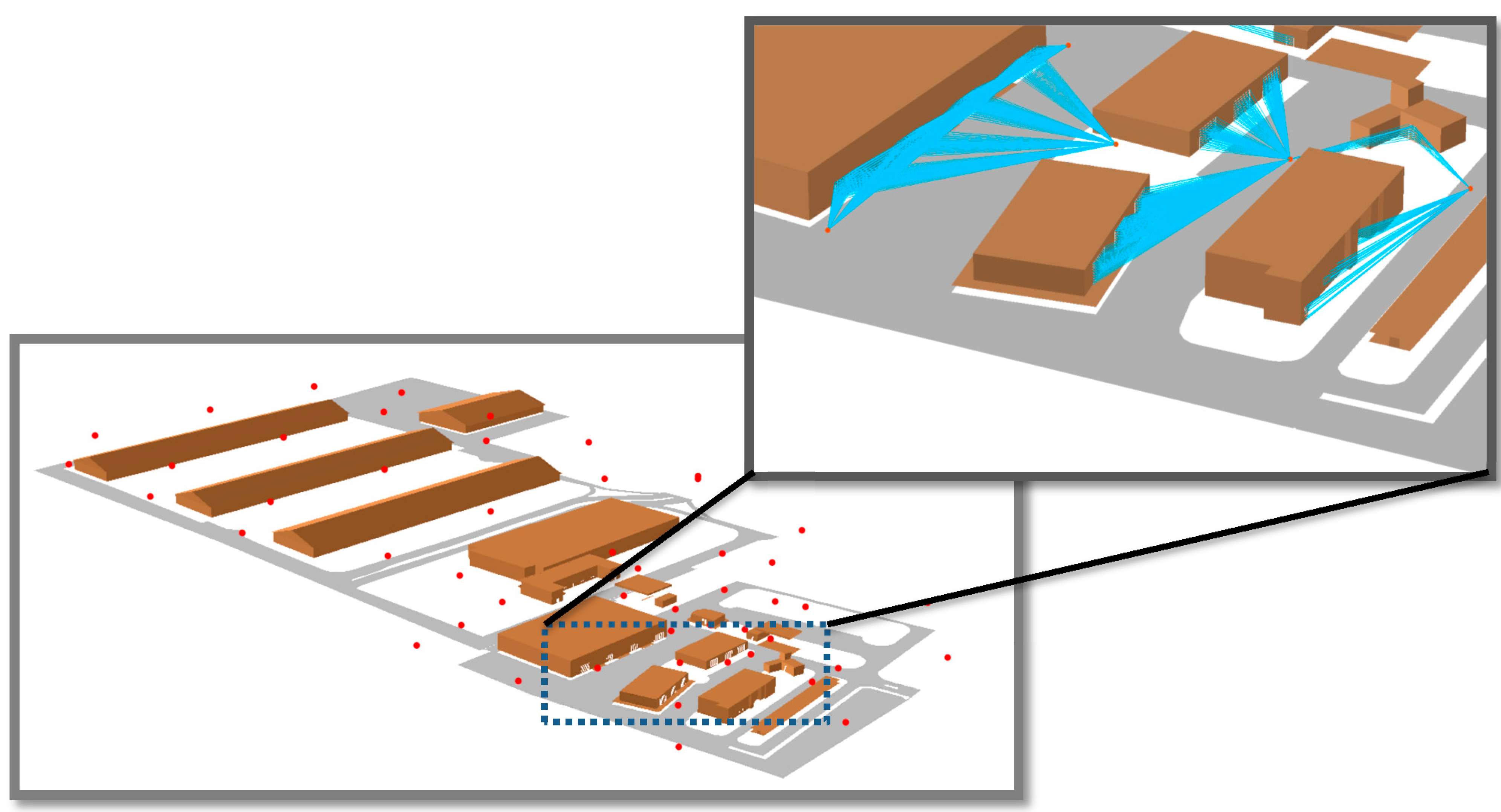
The last phase in implementing the HybVOR approach is performing the 3D Vector-based analysis of visibility. The objective of this step is to ensure that the main entrances of buildings (doors, windows, etc.) are fully monitored from the proposed location of cameras. In the case where some entrances are not entirely visible, the position of the corresponding cameras is manually changed in order to improve the visibility (minor displacements that do not affect the surface coverage are carried out). Figure 21 illustrates the results of our 3D Vector-based analysis of visibility based on HybVOR approach.

Figure 21. 3D Vector-based analysis of visibility based on HybVOR approach.

Figure 21. 3D Vector-based analysis of visibility based on HybVOR approach.

6.3. Discussion

In this case study, the HybVOR approach is implemented in order to find the optimal placement of camera network in a region of interest within the Jeddah Seaport. The proposed location of cameras is based on Voronoi diagram generated from buildings’ footprint. The use of the Voronoi diagram to place the camera network allows determining an optimal number of cameras for an almost complete coverage. The results of our implementation show that the optimal number of cameras is 48 cameras over an area of 0.1336 km². A surface coverage of almost 100% is obtained based on the raster based viewshed calculation (surface of visible zones = 0.13 km², surface of non-visible zones = 0.036 km², where the non-visible zones mainly correspond to some buildings’ surfaces). Then, the 3D Vector-based analysis of visibility is used to ensure that the main buildings’ entrances are fully covered by the camera network.

It is important to mention that the number of cameras strongly depends on the characteristics of cameras used for monitoring the environment. The HybVOR approach takes into consideration this aspect through the database which is used to store the relationship among cameras and buildings’ entrances (Figure 14). In addition, this database supports the use of cameras with different properties within the same network.

At the moment, the implemented HybVOR approach requires some manual intervention in order to ensure a complete coverage for the main buildings’ entrances when performing the 3D Vector-based analysis of visibility. However, it is possible to automate this process through an Agent Based Modeling (ABM) process. In this case, each camera will be considered as an agent, where the initial location can be deduced from the HybVOR methodology. Then, these agents (cameras) can change their position, with some minor displacements, in order to resolve any issue related to a lack of coverage. The rules that constrain these ABM process have to respect the HybVOR approach. Such an improvement of the HybVOR approach will be the subject of future research work.

7. Conclusion and Future Works

In this paper, the principles of an innovative camera surveillance network placement approach named “HybVOR” are presented. This approach aims to provide the best placement of a monitoring surveillance network, while optimizing the number of cameras to be deployed. The idea behind HybVOR is to generate a Voronoi Diagram from buildings’ footprint and to use the Voronoï edges to place cameras of surveillance. Then, in order to assess the quality of the network coverage, we have combined; (1) a raster based viewshed calculation that uses a raster Digital Surface Model of the study region with (2) a 3D vector based analysis of visibility that relies on a 3D model containing the main entrances of buildings to be monitored. This combination of raster and vector visibility analysis increases the effectiveness of assessing the level of coverage expected from deploying the surveillance camera network.

The obtained results are very interesting in terms of providing an almost complete surface coverage, while choosing the locations of cameras that offer a full monitoring of the main entrances of buildings in addition to optimizing the number of deployed cameras. Our further investigations will focus on solving the automatic displacement of cameras resulting from our proposed method to resolve any lack of coverage. To achieve this goal, an Agent Based Model (ABM) will be developed; it aims to automate the displacement process without the need for manual intervention especially when performing 3D vector based analysis of visibility. This ABM will be based on the rules and constraints that come from placement principles of the HybVOR approach.

Finally, it is important to mention that the HybVOR approach is also useful for monitoring other elements of an urban landscape such as traffic movement and people surveillance. HybVOR is an appropriate method for placing cameras to monitor areas with high security interest. In addition, our proposed approach may be very effective for the deployment of mobile cameras that may be mounted on UAVs (Unmanned Aerial Vehicles). The configuration of such a network can be performed on the fly depending on the dynamic of the environment, the number of available UAVs and the importance of specific targets.