
Categorization and Conversions for Indexing Methods of Discrete Global Grid Systems


Abstract
: Digital Earth frameworks provide a tool to receive, send and interact with large location-based datasets, organized usually according to Discrete Global Grid Systems (DGGS). In DGGS, an indexing method is used to assign a unique index to each cell of a global grid, and the datasets corresponding to these cells are retrieved or allocated using this unique index. There exist many methods to index cells of DGGS. Toward facility, interoperability and also defining a “standard” for DGGS, a conversion is needed to translate a dataset from one DGGS to another. In this paper, we first propose a categorization of indexing methods of DGGS and then define a general conversion method from one indexing to another. Several examples are presented to describe the method.1. Introduction
Digital Earth frameworks provide a multiresolution representation of the Earth as a spatial reference model with the ability to visualize, retrieve, embed and analyze data at different levels of detail [1]. To assign data to locations and establish a multiresolution representation, the surface of the Earth is discretized using different methods. The traditional method of discretizing the Earth is to use a latitude/longitude (lat-long) parametrization of the sphere. Taking equal length steps along the latitudes and longitudes parametrizes the Earth into quadrilateral cells. These cells have difference sizes and become smaller approaching the poles. In addition, poles are singularities in the lat-long parametrization, and cells incident to the poles are triangular.
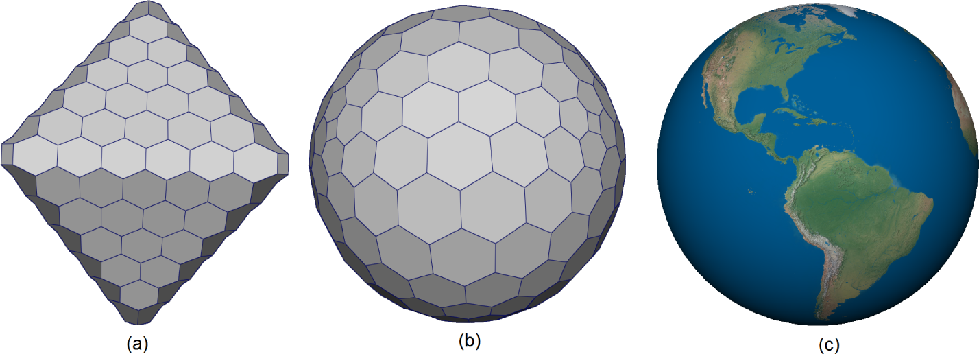
To obtain a more uniform cell structure with lower areal and angular distortions in order to simplify data analysis, Discrete Global Grid Systems (DGGS) have been proposed [1,2]. In DGGS, the Earth is approximated by a spherical (or ellipsoidal) polyhedron. Faces of the spherical polyhedron are refined by a specific factor of refinement (aperture) to provide a multiresolution representation. The refined faces of the polyhedron are then projected to the sphere to create cells on the surface of the Earth (see Figure 1). To assign datasets to these cells, a data structure is needed. In DGGS, typically, an indexing method is used to assign and retrieve and also handle essential queries. As a result, DGGS differ based on their initial polyhedron, cell type, projection and indexing method. These DGGS need to communicate and receive, share and integrate data coming from other DGGS. In essence, interoperability is an important property for these systems particularly in the context of the Open Geospatial Consortium (OGC). Conversion between DGGS is a crucial requirement for supporting this property. In this paper, we introduce a general conversion method for DGGS. This conversion can be potentially used from a DGGS to a future standard of a DGGS or an OGC standard. Since datasets are associated with DGGS through an indexing method, the conversion is essentially defined on the indexing methods if both DGGS use the same projection. For the general case, the projections are also needed to find the conversion. In the following, we initially discuss DGGS and its elements and then provide the general conversion for the indexing methods in Section 3.
1.1. Polyhedron
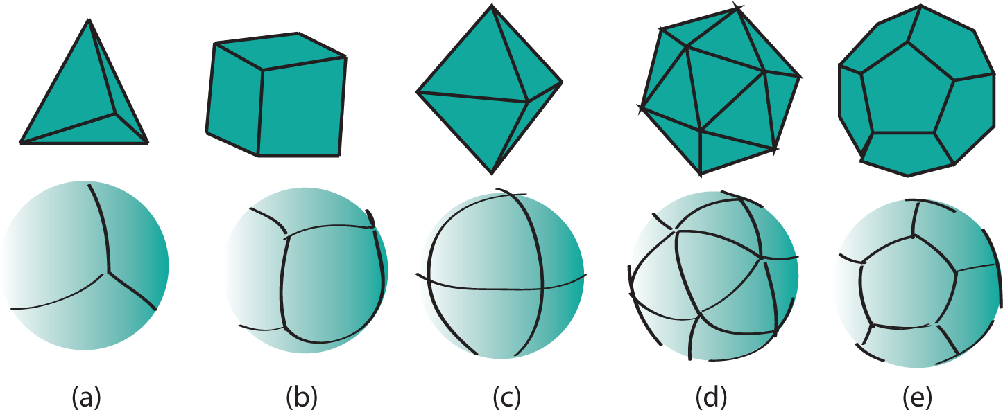
Different polyhedrons have been used in DGGS. Among the proposed polyhedrons for DGGS, the icosahedron has been widely used, as it can initially approximate the sphere with less angular and areal distortion [3–8] (see Figure 2d). Cubes are also widely used, as they provide quadrilateral cells that can be efficiently handled (see Figure 2b) [9–12]. Although tetrahedrons may cause noticeable angular and areal distortions in their approximations of the Earth, they remained a popular choice due to their simplicity [13] (see Figure 2a). Octahedrons are also very popular in representing the Earth, since their faces can be associated with spherical octants when their singular vertices can be placed at the poles [14–16] (see Figure 2c). Dodecahedrons have also been used (see Figure 2e). However, since the faces of the dodecahedron are pentagons and a pentagonal refinement does not exist, it has not been widely used in DGGS, although it introduces a reasonably low distortion [17].
1.2. Cell Type
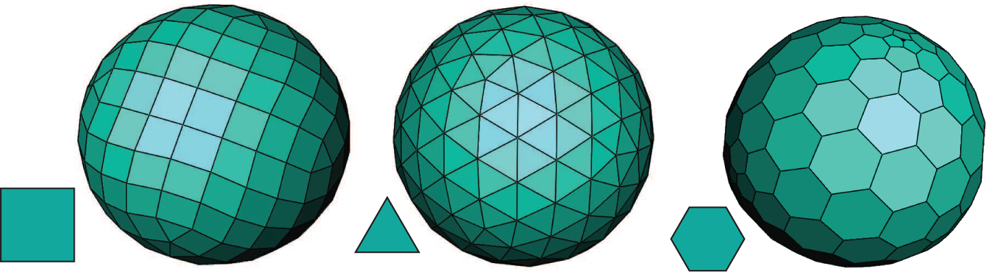
Quadrilateral, triangular and hexagonal cells are typically used in DGGS (see Figure 3). Quadrilateral cells are naturally used in DGGS using cubes as the polyhedron [9,10,12]. The congruency of quadrilateral cells paired with their adaptability to Cartesian coordinate systems, hardware devices and available data structures (such as quadtrees) make it a popular choice. However, since the commonly-used polyhedrons in DGGS initially have triangular faces, triangular cells are also widely used in DGGS [13,14,18,19]. These cells are also congruent, and they can be rendered very efficiently, as they are supported by many built-in functions in rendering pipelines, such as OpenGL. Conceptually, the triangular cells in polyhedrons with triangular faces, such as the octahedron and icosahedron, can also be paired into quadrilateral (diamond) cells [8]. Hexagonal cells are created on polyhedrons with triangular faces by applying a dual conversion to the triangular faces [20]. Hexagonal cells are also popular, as they are efficient in sampling, and they exhibit a uniform adjacency [5–8,15,16,20–22].
1.3. Refinement (Aperture)
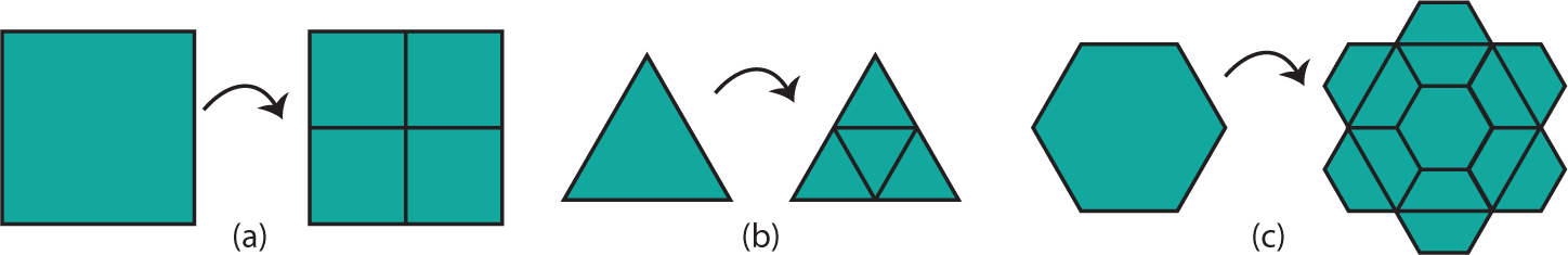
Converting a set of coarse cells to finer cells through splitting edges or shrinking cells is called refinement. Consider the cells of a planar lattice. If a cell with area A is subdivided by refinement R to a set of cells with area , refinement R is said to be a one-to-i refinement with a factor (aperture) of i (see Figure 4). A refinement with a lower factor of refinement is usually desired, as it can generate a greater number of resolutions under a fixed number of maximum cells and, therefore, provides a smoother transition between resolutions [10]. Of the quadrilateral refinements, one-to-two, one-to-four and one-to-nine refinements have been used so far [9,10,12]. For triangular refinements, one-to-four refinement is the most commonly used [13,14,18,19,23], while hexagonal refinements have employed in one-to-three [6,7], one-to-four [16,22] and one-to-seven variations [24].
1.4. Projection
Spherical projections have been studied for a long time in the field of cartography [25]. When the faces of a polyhedron are projected onto the sphere, two types of distortions may be created: angular distortion or areal distortion [26]. There exists a trade-off between these two distortions. This means that reducing one type of distortion causes greater distortion of the other. If a spherical projection preserves the area, it is equal area projection, and if it preserves the angles, it is angular preserving or conformal. Equal area projections are typically more desirable in DGGS, as they simplify data analysis [2,6,10,11,22]. In the frameworks proposed in [2,6,22], Snyder equal area projection has been used, which is a popular projection due to its low angular distortion and the mapping of edges of the polyhedron to great circle arcs [27]. However, other types of equal area projection have also been used due to their own desirable properties, such as providing closed forms for both projection and inverse projection [10,28].
1.5. Indexing Methods
To assign data, traverse between resolutions and handle essential queries in DGGS, a data structure is needed. Hierarchical data structures, such as quadtrees, may seem to be an obvious choice [29,30]. However, to interactively work with huge data on the fly, an indexing method is needed that can discard the tree structure requiring many pointers to maintain the connectivity. Many indexing methods have been proposed for DGGS. In the following sections, we first categorize the proposed indexing methods for DGGS, and then, in Section 3, we provide a framework to convert an index from one DGGS to another. Note that if each of the elements listed above (i.e., projection, factor of refinement, type of cell and polyhedron) is different from one DGGS to another, the indices do not refer to the same point on the Earth. However, we can convert the indices to each other and anticipate the resulting error of the conversion process.
2. Indexing Categorization
Given an indexing method of a DGGS, it is desired that each cell at each resolution receives an index i that uniquely identifies the cell. From the index of a cell, its location (typically its centroid) on the Earth and also the resolution of the cell is determined. The index of a cell may also refer to a data structure or database to retrieve data associated with the cell. The indices of cells can be 1D (a string of letters and digits) or they can be nD, resulting from n axes defined on the faces of a polyhedron. Although various types of indexing exist to index cells of DGGS, they are typically derived from three types of general indexing mechanisms: we call indexing methods that benefit from the hierarchy of cells provided by the refinement hierarchy-based indexing methods. In some indexing methods, the parameterization provided by a space-filling curve is used to index cells. Using the axes of a coordinate system defined on the cells of a polyhedron is also another common method, that we call axes-based indexing. In the following, we describe each category and provide some existing examples.
2.1. Hierarchy-Based Indexing
Applying refinements on a polyhedron produces a useful hierarchy between cells that can be used to index cells. When a refinement is applied on a set of coarse cells C, a set of fine cells F is created. We can assign each cell f ∈ F to a unique cell c ∈ C. In this case, f is the child of c.
As discussed earlier, it is possible to index the cells using the defined hierarchy. We can initially index the first resolution cells and then use this index as the prefix of the index at the following resolutions. Formally, if cell c has index I, its children fi receive index Ii in which i is an integer digit appended to I. The range of i is denoted by b (i.e., i ∈ [0, b − 1]) which is used as the base of this indexing method. This base can be used to define algebraic operations on indices, such as conversion to and from the Cartesian coordinate system, neighborhood finding and Fourier transform [2,7,19].
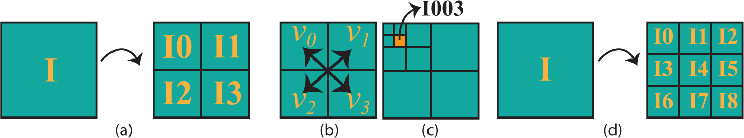
An example of this indexing is proposed in [31] for quadrilateral cells resulting from a one-to-four refinement. As a result, the children resulting from one-to-four refinement of a quad with index I receive indices I0 for the NW cell, I1 for the NE cell, I2 for the SW cell and I3 for the SE cell (Figure 5a). An index with length r corresponds to a cell at resolution r whose location is determined using the vector obtained from the sequence of digits. Figure 5b shows the vectors associated with each digit. The vector associated with an index is an addition of scaled vectors associated with each digit. For example, the cell with index I003 is obtained after applying one-to-four refinement three times on cell I. The vector associated with this index is obtained by (Figure 5b,c). SCENZ-Grid [12] also uses similar indexing method for one-to-nine refinement of the quadrilateral faces of a cube in which the digit appended to the index of a fine cell varies between zero and eight based on its relative position to its parent (Figure 5d).
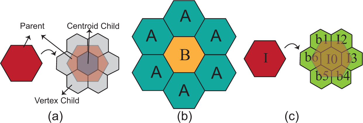
For congruent refinements, this hierarchical relationship between the cells is trivial, as the parent encloses all its children (Figure 4a,b). However, for incongruent refinements, such as hexagonal refinements (Figure 4c), assigning a set of fine cells to a unique coarse cell is not trivial. PYXIS indexing [7] is defined on hexagonal cells resulting from one-to-three refinement on an icosahedron. Under this indexing, children are categorized into centroid children and vertex children (see Figure 6a). Centroid children share a centroid with their parent, while vertex children are covered by three different coarse hexagons, each of which could potentially be defined as the parent. Coarse hexagons are categorized into two categories, A and B, in which each type B cell is surrounded by type A cells (see Figure 6b). Each type B cell is treated as the parent of its centroid child and all its vertex children while type A cells are only considered as the parent of their centroid child. Afterwards, each centroid child is considered to be type B and each vertex child is considered to be type A, and the process continues and produces a fractal shape. This indexing is started from a truncated icosahedron (the refined icosahedron by the one-to-three refinement). In the truncated icosahedron, the initial pentagons are type B cells, while hexagons are type A cells. If a coarse cell has index I, its centroid child gets indices I0 and its vertex children get index Ii in which 1 ≤ i ≤ 6 (see Figure 6c). Since each fine cell receives the index of its parent as the prefix, PYXIS indexing is a hierarchy-based indexing method.
There exist many other hierarchy-based indexing methods in DGGS [11,14,19,22,23]. In [11], a hierarchy-based mechanism is used on the quadrilateral faces of a cube that are refined by a factor of four. Triangular cells resulting from a one-to-four refinement are indexed similarly in [14,19,23], and in [22], the hexagonal cells of an icosahedron resulting from a one-to-four refinement are indexed with a similar mechanism.
2.2. Space-Filling Curve Indexing
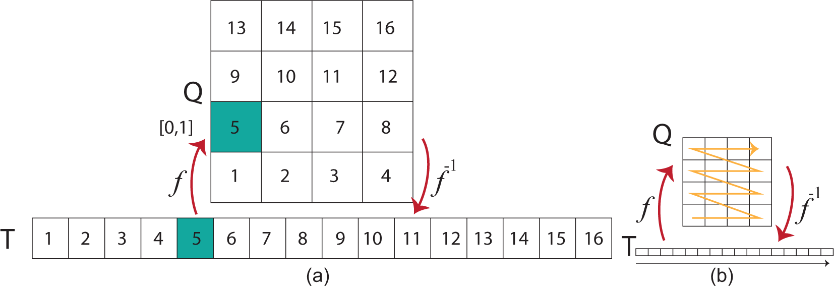
Another method of indexing cells in DGGS is to use space-filling curves (SFCs) as a reference. SFCs have been used in many applications, such as compression, rendering and database management. SFCs are 1D curves that are created recursively to eventually cover a space. Space filling curve f(t) typically provides a mapping from T ⊂ R to Q ⊂ R2 in which t ∈ T (see Figure 7). Using an SFC that visits all of the cells of Q after refinement, we may define an indexing on the cells of Q by discretizing T based on the number of cells. The 1D index I for cells in Q is defined on domain T (i.e., by taking a unit step on T, I is incremented). Each index I has a corresponding cell on Q that is returned by the mapping f (f(I) ∈ Q). Given mapping f from T to Q, f−1, which maps the cells of Q to their unique index defined on T, can also be defined. Figure 7 illustrates an example of an indexing for Q based on a SFC, which is simply a row major traversal.
Based on the properties that function f exhibits, different SFCs have been proposed. Some of the common SFCs are Hilbert, Peano, Sierpinski and Morton (Z), as illustrated in Figure 8. As noticeable in Figure 8, these curves typically have a simple initial geometry defined on a simple domain. The domain is then refined, and the simple geometry is repetitively transformed to cover the entire refined domain. For instance, in the case of the Hilbert curve, the simple geometry is defined on a simple two by two domain, and the domain is then refined by a one-to-four refinement. Typically, if the initial geometry covers i cells, a one-to-i refinement is suitable to get a refined domain. This way, each SFC is associated with a refinement.
To index cells based on an SFC, decimal numbers may not be the best choice, as their corresponding indices do not directly provide any information about the resolution. As a result, a base b for the indexing may be chosen to solve this issue. The base of the indexing method is usually chosen as i or if refinement one-to-i is associated with the SFC curve. In this case, given an index with base i, a cell at resolution n has an index, whereas, given a base of , the cell receives an index of length 2n. In addition, using these bases, redundant bits are not necessary to index cells, since whole cells resulting from these refinements can be covered by indices from 00…0 to (b − 1)…(b − 1).
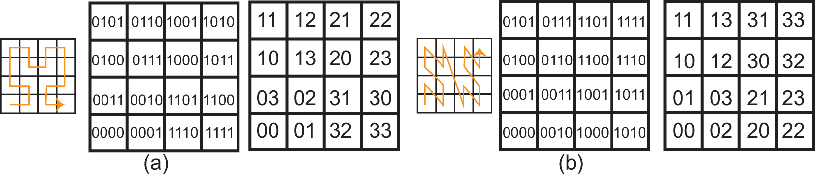
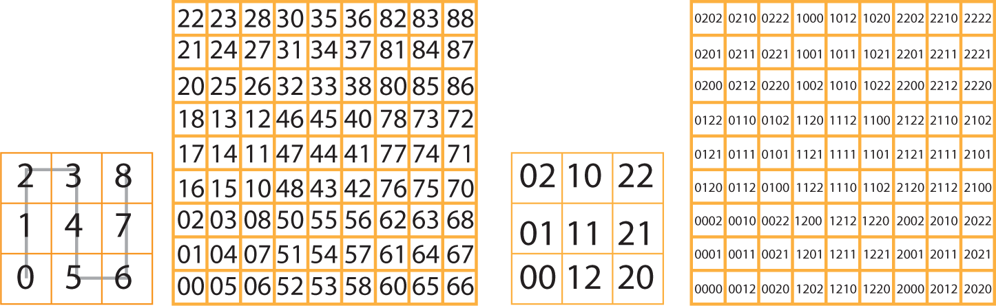
For instance, the refinement associated with the Hilbert and Morton curves is one-to-four. Therefore, base four or two for Hilbert and Morton is appropriate. After fixing a base for the index, the cell associated with the initial point of the curve gets index zero. As we move along the SFC, the index of each subsequent cell is incremented by one in base b. Figure 9 illustrates such an indexing for the Hilbert and Morton curves using bases two and four. Although base four seems to be more efficient, as it provides a shorter string to index cells, indices with base two can also be implemented efficiently, as they are compatible with efficient binary operations in hardware.
Indexing methods derived from SFCs have been widely used in DGGS and terrain rendering. For instance, in [8,32], Morton indexing has been used to index cells resulting from one-to-four refinements on the icosahedron and octahedron, while in [18], the Sierpinski SFC has been used to index triangular cells. SFCs used in terrain rendering provide a 1D ordering of triangle strips and vertices suitable for GPU and out-of-core algorithms [33–36].
2.3. Axes-Based Indexing
A natural way for indexing is to define a set of m axes U1 to Um to span the entire space on which the cells lie. Then, the index would be an m-dimensional vector (i1, i2, …, im) in which ij are integer numbers indicating unit steps taken along the axes Uj. A simple example of such an indexing is to index a quadrilateral domain by Cartesian coordinates, as illustrated in Figure 10a. When a refinement is applied to the cells, a subscript r is appended to the index indicating the resolution [20,37,38]. In the available indexing methods for DGGS, m is typically two or three. For instance, 2D indexing has been used in [5,10,20], while 3D indexing has been used in [15,16] by taking the barycentric coordinate of each cell to be its index. To apply a 2D indexing method on a polyhedron for DGGS, the polyhedron can be unfolded to a 2D domain and the axes defined for the entire 2D domain or each face can be given its own coordinate system [20,37,38]. Figure 10 illustrates an indexing for the quadrilateral cells of a cube after one-to-four refinement, wherein each face has its own coordinate system. To distinguish between the cells associated with each face, an additional component referring to the initial number of the polyhedron’s faces can be added to the indices. As a result, index [f, (a, b)r] refers to cell (a, b) in face f at resolution r (Figure 10d).
The provided categorization mostly reflects the core idea for constructing indexing methods. According to this categorization/construction, some of the operations can be naturally handled. For example, hierarchy-based indexing methods naturally led to efficient parent-child operations. However, it is necessary to consider other properties and operations for well-designed indexing methods. Certainly, it is possible to handle neighborhood finding in hierarchy-based indexing methods, but probably not as efficient/natural as axes-based techniques. In addition, based on the pattern of indices, some indexing methods can belong to two categories (e.g., SFC or hierarchy-based). However, an indexing method is either constructed by a parametrized SFC or by inheriting the index of its parent. Although it is possible to use a parametrized SFC that indexes the children by indices that have the prefix of their parents, the indexing method is SFC since the construction of indexing is based on the parameterization of SFC.
3. General Conversion Method
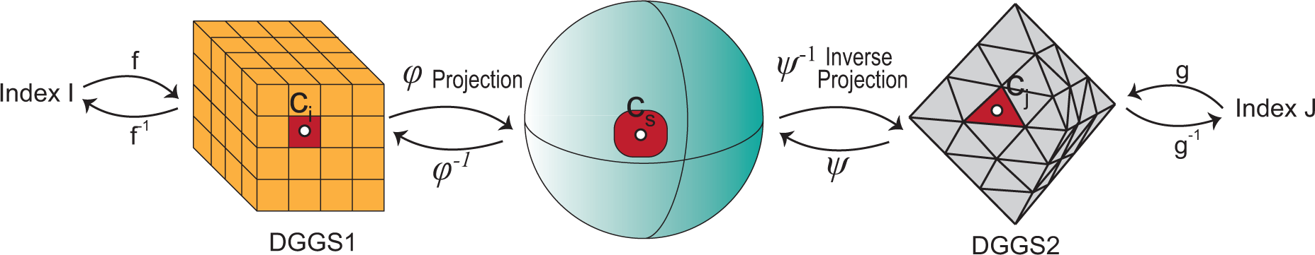
As discussed earlier, there exist many different Digital Earth frameworks resulting from various types of DGGS. However, data in these frameworks are essentially assigned to the index of each cell. Indexing methods for different DGGS may be different from each other. In order to exchange, unify or standardize data represented in different frameworks, a conversion is necessary that can convert an index in one type of DGGS to another. Consider index Iin DGGS1; we would like to know the index J in DGGS2 that is referring to “almost the same area”. Since each cell is composed of a point and an area that has been enclosed by that cell on the sphere (or ellipsoid), if any component of the DGGS (type of cell, polyhedron, indexing, aperture and projection) differs between DGGS1 and DGGS2, the index of a cell in DGGS1 refers to a different area on the sphere (ellipsoid) compared to an index in DGGS2. To define such a conversion between different frameworks, we can benefit from a common domain for two DGGS. This domain can be a spherical/ellipsoidal or 2D Cartesian corresponding to faces of the polyhedron (see Figure 11). As a result, we discuss two cases for conversions in the following.
Case 1 (General Case): Consider that, in addition to different indexing methods, at least another component of DGGS1 is different from DGGS2. In this case, we use a common spherical domain to convert index I in DGGS1 to index J in DGGS2. Consider I in DGGS1 and ci the centroid of its corresponding cell in DGGS1. The face corresponding to this index on the refined polyhedron of DGGS1 is found by the mapping f. Note that functions f and f−1 are readily available in most DGGS, since they are essential queries to relate an index to its position on the polyhedron and vice versa. We can then project this point to point cs on the sphere, using the projection φ used in DGGS1. cs can be inversely projected to point cj on DGGS2 using the inverse projection ψ−1 in DGGS2. The index J of the cell enclosing cj in DGGS2 is the desired index, which can be obtained by the mapping g−1 (see Figure 11). Note that g maps an index to a point on a polyhedron, while g−1 maps a point to an index of a cell enclosing the point at a specific resolution.
There exists an ambiguity here about the resolution of indices. The resolution of index I is given. However, the resolution of index J should be determined. To do this, we take the resolution for J at which the area of cells corresponding to I and J are as close as possible. For instance, if a cell has an index at resolution seven in PYXIS indexing, the corresponding index on the cube after one-to-nine refinement (as in SCENZ-Grid) will be at resolution five, while the index on the cube after one-to-four refinement will be at resolution seven. Table 1 lists the number of cells in these frameworks, which is used to evaluate the areas of the cells at each resolution. Consequently, if cell I in DGGS1 has area Ai, resolution r in DGGS2 is chosen in which Minr |Ar − Ai| is satisfied (i.e., the resolution is chosen in which the areas of the cells (Ar) are closest to Ai).
Case 2: The conversion is easier when all components of DGGS1 and DGGS2 are the same except for the indexing methods; hence, ψ = φ and the resolutions are the same. As a result, we can easily use functions f and g that map an index to a polyhedron. In this case, the indices are either in the first two categories (SFC or hierarchy-based) and as a result are 1D indices or they are integer vectors defined in an axes-based indexing method. In both cases, we can convert the index of one category to a vector and convert the vector to an index in another category.
Functions f and g are usually found by determining the corresponding 2D vectors of each index. To describe this conversion, we use an example. Consider the cells of one-to-nine refinement on the cube with the hierarchy-based indexing used in SCENZ-Grid (see Figure 5) and an axes-based indexing using Cartesian coordinates (Figure 12a,b). A cell with index N000 is given, and its corresponding index in the axes-based indexing system is desired. As illustrated in Figure 12, digit zero in the hierarchy-based indexing system corresponds to vector (−1, 1) in the Cartesian coordinate system. Note that as cells get smaller by a factor as the resolution increases, the length of this vector is also scaled by (Figure 12c,d). As a result, 000 in the hierarchy-based indexing corresponds to the addition of vectors (−1, 1), (−1, 1) and (−1, 1), which is equivalent to . To get integer indices, we only need to scale the coordinate by nine; therefore, the index corresponding to N000 is [N, (−13, 13)2] (N refers to one of the initial faces of the cube).
The complexity of both of the conversion methods proposed in this paper is dependent on the employed functions, f, g, ϕ and ψ, and their inverses. These functions are typically computed in constant time or very efficiently, as the performance of the DGGS is dependent on these functions. As a result, the performance of our proposed conversion is proportional to the performance of f, g, ϕ and ψ.
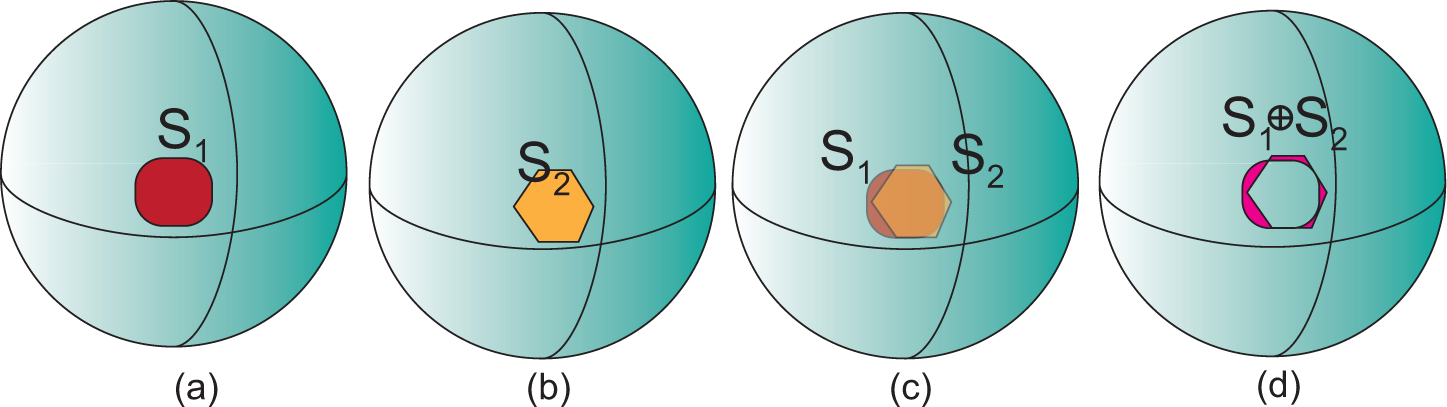
When the cells in these DGGS differ, any conversion introduces an error. Therefore, while no error will be introduced in the second case, there will be some error in the first case, as the cells represented by two indices may be different in shape and size. Since each index represents an area on the surface of the Earth, this error can be measured as the difference between the areas that the two cells are covering (see Figure 13). Indeed, if S1 and S2 are, respectively, sets of points on the surfaces of DGGS1 and DGGS2, the error can be measured by the symmetric difference of these two subsets (S1 ⊕ S2).
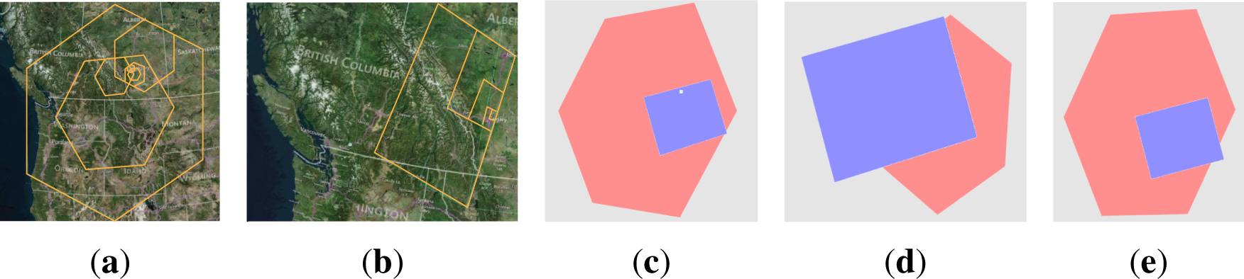
To provide an example of our proposed conversion, we have implemented it for converting from PYXIS to Cube(one-to-four). In the Cube (one-to-four) framework, the equal area projection discussed in [28] has been used with a one-to-four refinement. As discussed earlier, we can determine resolutions for which PYXIS cells and Cube (one-to-four) cells are more compatible based on the area of cells. For instance, PYXIS cells at resolutions three, six and seven correspond to cells of Cube (one-to-four) at resolutions four, six and seven, respectively. Hexagonal cells in the PYXIS framework are converted to quadrilateral cells in Cube (one-to-four), illustrated in Figure 14 (textures are removed to increase the visibility). After converting hexagonal cells into quadrilateral cells, it is shown that hexagonal cells and quad cells share an area with factors of 15%, 48% and 18% at resolutions three, six and seven, respectively. This conversion is performed in real time (less than milliseconds) at any resolution, as projections and inverse projections of both of the frameworks are very fast and efficient.
Using the conversions proposed in this section, we can simply convert indices from one type of DGGS to another. This work also clarifies that various types of indexing methods can be proposed for a DGGS. However, most methods fall under one of the categories proposed in this paper. For instance, it is possible to define another indexing method for SCENZ-Grid using the Peano SFC considering two different bases, three and nine (see Figure 15). As a result, our work can serve as useful material for researchers looking to design an indexing method for a potential OGC standard working based on DGGS.
4. Conclusions
In this paper, we provide a categorization of indexing methods proposed for Digital Earth frameworks. We then proposed a conversion from one category to another. This shows that data allocated to cells can be represented in different ways using different types of DGGS and that there exists a simple conversion between these representations that can be used to unify the data available given any DGGS. This work also clarifies a method to index potentially new DGGS with a specific type of cell and aperture.
Using our proposed conversion, current DGGS that are employed in research or industrial settings can communicate, share and receive data from each other or a potential OGC standard. As a result, our work facilitates the interoperability of DGGS. In addition, using our proposed categorization, it is possible to propose alternative indexing mechanisms for an established DGGS.
There remain some possible directions for future work regarding this subject. In this paper, we focus mostly on DGGS that employ an equal area projection. However, other types of projections may be used. In that case, the areas of the cells are not equal even within a specific resolution. Hence, when converting the index of a cell, the conversion will need to locate the cell that has the closest area to the target cell. More research is needed to determine an efficient method for choosing the appropriate resolution at which to locate this cell.
Acknowledgments
We would like to thank Idan Shatz, Logan Rakai, and Nader Hamekasi for their support and insightful discussions. We also thank Troy Alderson for proofreading and editorial comments. This research has been partially supported by National Science and Engineering Research Council of Canada (NSERC) and PYXIS Innovation Inc.
Author Contributions
Ali Mahdavi-Amiri, and Faramarz Samavati developed the methodology and performed the experiments.
Ali Mahdavi-Amiri, Faramarz Samavati, and Perry Peterson analyzed the methodology.
Ali Mahdavi-Amiri, Faramarz Samavati, and Perry Peterson wrote the paper.
Conflicts of Interest
The authors declare no conflict of interest.
References
- Goodchild, M.F. Discrete global grids for Digital Earth, Proceedings of the 1 st International Conference on Discrete Global Grids, Santa Barbara, CA, USA, 26–28 March 2000.
- Sahr, K.; White, D.; Kimerling, A.J. Geodesic discrete global grid systems. Cartogr. Geogr. Inf. Sci. 2003, 30, 121–134. [Google Scholar]
- Tong, X.; Ben, J.; Qing, Z.; Zhang, Y. The hexagonal discrete global grid system appropriate for remote sensing spatial data. Proc. SPIE. 2000, 7146. [Google Scholar] [CrossRef]
- Tong, X.; Ben, J.; Wang, Y.; Zhang, Y.; Pei, T. Efficient encoding and spatial operation scheme for aperture 4 hexagonal discrete global grid system. Int. J. Geogr. Inf. Sci. 2013, 27, 898–921. [Google Scholar]
- Sahr, K. Location coding on icosahedral aperture 3 hexagon discrete global grids. Comput. Environ. Urban Syst 2008, 32, 174–187. [Google Scholar]
- Peterson, P. Close-Packed, Uniformly Adjacent, Multiresolutional, Overlapping Spatial Data Ordering. U.S. Patent US 20,060,265,197 A1, 23 November 2006. [Google Scholar]
- Vince, A.; Zheng, X. Arithmetic and Fourier transform for the PYXIS multi-resolution digital Earth model. Int. J. Digit. Earth. 2009, 2, 59–79. [Google Scholar]
- White, D. Global grids from recursive diamond subdivisions of the surface of an octahedron or icosahedron. Environ. Monit. Assess. 2000, 64, 93–103. [Google Scholar]
- Alborzi, H.; Samet, H. Augmenting SAND with a spherical data model, Proceedings of the First International Conference on Discrete Global Grids, Santa Barbara, CA, USA, 26–28 March 2000.
- Mahdavi-Amiri, A.; Bhojani, F.; Samavati, F. One-to-Two Digital Earth. In Advances in Visual Computing, Lecture Notes in Computer Science, Proceedings of 9th International Symposium on Visual Computing, Rethymnon, Crete, Greece, 29–31 July 2013; Bebis, G., Boyle, R., Parvin, B., Koracin, D., Li, B., Porikli, F., Zordan, V., Klosowski, J., Coquillart, S., Luo, X., et al, Eds.; Springer: Berlin, Germany, 2013; pp. 681–692. [Google Scholar]
- Górski, K.M.; Hivon, E.; Banday, A.J.; Wandelt, B.D.; Hansen, F.K.; Reinecke, M.; Bartelmann, M. HEALPix: A framework for high-resolution discretization and fast analysis of data distributed on the sphere. Astrophys. J. 2005, 622, 759–771. [Google Scholar]
- Gibb, R.; Raichev, A.; Speth, M. The rHEALPIX Discrete Global Grid System, Available online: http://raichev.net/files/rhealpix_dggs_preprint.pdf accessed on 15 January 2013.
- Cozzi, P.; Ring, K. 3D Engine Design for Virtual Globes, 1st ed.; Peters, A. K., Ed.; Ltd: Natick, MA, USA, 2011. [Google Scholar]
- Dutton, G. A Hierarchical Coordinate System for Geoprocessing and Cartography: With 85 Figures, 16 Tables and 2 Foldouts. In Lecture Notes in Earth Sciences Series; Springer-Verlag: Berlin, Germany, 1999. [Google Scholar]
- Vince, A. Indexing the aperture 3 hexagonal discrete global grid. J. Vis. Commun. Image Represent 2006, 17, 1227–1236. [Google Scholar]
- Ben, J.; Tong, X.; Chen, R. A spatial indexing method for the hexagon discrete global grid system, Proceedings of the 2010 18th International Conference on Geoinformatics, Beijing, China, 18–20 June 2010; pp. 1–5.
- Wickman, F.E.; Elvers, E.; Edvarson, K. A system of domains for global sampling problems. Geogr. Ann. Ser. A Phys. Geogr. 1974, 56, 201–212. [Google Scholar]
- Bartholdi, J.J., III; Goldsman, P. Continuous indexing of hierarchical subdivisions of the globe. Int. J. Geogr. Inf. Sci. 2000, 15, 489–522. [Google Scholar]
- Goodchild, M.F.; Shiren, Y. A hierarchical spatial data structure for global geographic information systems. CVGIP: Graph. Models Image Process 1992, (54), 31–44. [Google Scholar]
- Mahdavi-Amiri, A.; Harrison, E.; Samavati, F. Hexagonal connectivity maps for Digital Earth. Int. J. Digit. Earth. 2014. [Google Scholar] [CrossRef]
- Sahr, K. Hexagonal discrete global grid systems for geospatial computing. Arch. Photogramm. Cartogr. Remote Sens 2011, 22, 363–376. [Google Scholar]
- Tong, X.; Ben, J.; Wang, Y.; Zhang, Y.; Pei, T. Efficient encoding and spatial operation scheme for aperture 4 hexagonal discrete global grid system. Int. J. Geogr. Inf. Sci. 2013, 27, 898–921. [Google Scholar]
- Szalay, A.S.; Gray, J.; Fekete, G.; Kunszt, P.Z.; Kukol, P.; Thakar, A. Indexing the Sphere with the Hierarchical Triangular Mesh; TechReport MSR-TR-2005-123; Microsoft Research: Redmond, WA, USA, 2005. [Google Scholar]
- Gibson, L.; Lucas, D. Spatial data processing using generalized balanced ternary, Proceedings of the IEEE Computer Society on Pattern Recognition and Image Processing, Las Vegas, NV, USA, 14–17 June 1982; pp. 566–572.
- Kennedy, M.; Koop, S. Environmental Systems Research Institute. Understanding map projections: GIS by Esri. In ArcGIS 8 Concept Guides; Environmental Systems Research Institute: Redlands, CA, USA, 2000. [Google Scholar]
- Hormann, K.; Lévy, B.; Sheffer, A. Mesh parameterization: Theory and practice video files associated with this course are available from the citation page, Proceedings of the ACM SIGGRAPH 2007 Courses (SIGGRAPH ’07), Special Interest Group on Computer Graphics and Interactive Techniques Conference, San Diego, CA, USA, 5–9 August 2007.
- Snyder, J.P. An equal area map projection for polyhedral globes. Cartographica 1992, 29, 10–21. [Google Scholar]
- Roşca, D.; Plonka, G. Uniform spherical grids via equal area projection from the cube to the sphere. J. Comput. Appl. Math. 2011, 236, 1033–1041. [Google Scholar]
- Samet, H. Foundations of Multidimensional and Metric Data Structures (The Morgan Kaufmann Series in Computer Graphics and Geometric Modeling); Morgan Kaufmann Publishers Inc: San Francisco, CA, USA, 2005. [Google Scholar]
- Faust, N.; Ribarsky, W.; Jiang, T.; Wasilewski, T. Real-time global data model for the Digital Earth, Proceedings of the International Conference on Discrete Global Grid, Santa Barbara, CA, USA, 26–28 March 2000.
- Gargantini, I. An effective way to represent quadtrees. ACM Commun 1982, 25, 905–910. [Google Scholar]
- Bai, J.; Zhao, X.; Chen, J. Indexing of the discrete global grid using linear quadtree, Proceedings of ISPRS Hangzhou 2005 Workshop on Service and Application of Spatial Data Infrastructure, Hangzhou, China, 14–16 October 2005; pp. 267–270.
- Pharr, M.; Fernando, R. GPU Gems 2: Programming techniques for high-performance graphics and general-purpose computation. In Chapter Terrain Rendering Using GPU-Based Geometry Clipmaps; Addison-Wesley: Boston, MA, USA, 2005. [Google Scholar]
- Hwa, L.M.; Duchaineau, M.A.; Joy, K.I. Real-time optimal adaptation for planetary geometry and texture: 4-8 tile hierarchies. IEEE Trans. Vis. Comput. Graph. 2005, 11, 355–368. [Google Scholar]
- Lawder, J. The Application of Space-Filling Curves to the Storage and Retrieval of Multi-Dimensional Data. In Ph.D. Thesis; University of London: London, UK, 2000. [Google Scholar]
- Lindstrom, P.; Pascucci, V. Terrain simplification simplified: A general framework for view-dependent out-of-core visualization. IEEE Trans. Vis. Comput. Graph. 2002, 8, 239–254. [Google Scholar]
- Mahdavi-Amiri, A.; Samavati, F. Connectivity maps for subdivision surfaces, Proceedings of the GRAPP/IVAPP, Rome, Italy, 24–26 February, 2012; pp. 26–37.
- Mahdavi-Amiri, A.; Samavati, F. Atlas of connectivity maps. Comput. Graph. 2014, 39, 1–11. [Google Scholar]


| Resolution | PYXIS | SCENZ-Grid | Cube (1-to-4) |
|---|---|---|---|
| 1 | 32 | 6 | 6 |
| 2 | 92 | 54 | 24 |
| 3 | 272 | 486 | 96 |
| 4 | 812 | 5374 | 384 |
| 5 | 2432 | 39,366 | 1536 |
| 6 | 7292 | 354,294 | 6144 |
| 7 | 21,872 | 3,188,646 | 24,576 |
| 8 | 65,612 | 28,697,814 | 98,304 |
| 9 | 196,832 | 258,280,326 | 393,216 |
© 2015 by the authors; licensee MDPI, Basel, Switzerland This article is an open access article distributed under the terms and conditions of the Creative Commons Attribution license (http://creativecommons.org/licenses/by/4.0/).
Share and Cite
Amiri, A.M.; Samavati, F.; Peterson, P. Categorization and Conversions for Indexing Methods of Discrete Global Grid Systems. ISPRS Int. J. Geo-Inf. 2015, 4, 320-336. https://doi.org/10.3390/ijgi4010320
Amiri AM, Samavati F, Peterson P. Categorization and Conversions for Indexing Methods of Discrete Global Grid Systems. ISPRS International Journal of Geo-Information. 2015; 4(1):320-336. https://doi.org/10.3390/ijgi4010320
Chicago/Turabian StyleAmiri, Ali Mahdavi, Faramarz Samavati, and Perry Peterson. 2015. "Categorization and Conversions for Indexing Methods of Discrete Global Grid Systems" ISPRS International Journal of Geo-Information 4, no. 1: 320-336. https://doi.org/10.3390/ijgi4010320
APA StyleAmiri, A. M., Samavati, F., & Peterson, P. (2015). Categorization and Conversions for Indexing Methods of Discrete Global Grid Systems. ISPRS International Journal of Geo-Information, 4(1), 320-336. https://doi.org/10.3390/ijgi4010320