Holistics 3.0 for Health

Abstract

Human health is part of an interdependent multifaceted system. More than ever, we have increasingly large amounts of data on the body, both spatial and non-spatial, its systems, disease and our social and physical environment. These data have a geospatial component. An exciting new era is dawning where we are simultaneously collecting multiple datasets to describe many aspects of health, wellness, human activity, environment and disease. Valuable insights from these datasets can be extracted using massively multivariate computational techniques, such as machine learning, coupled with geospatial techniques. These computational tools help us to understand the topology of the data and provide insights for scientific discovery, decision support and policy formulation. This paper outlines a holistic paradigm called Holistics 3.0 for analyzing health data with a set of examples. Holistics 3.0 combines multiple big datasets set in their geospatial context describing as many areas of a problem as possible with machine learning and causality, to both learn from the data and to construct tools for data-driven decisions.

1. Introduction

For decades, experts in public health and the social sciences have recognized the geospatial variation of populations; health is shaped by multiple factors, including healthcare, public health systems, individual behaviors (e.g., smoking) and risk factors (e.g., obesity), socioeconomic factors (e.g., income, education), the physical environment (e.g., air pollution), the social environment (e.g., social support), public policies and the “macro-structural” elements of society that shape this entire list. Linking these data to resolve public health concerns requires accounting for non-linear multi-variate relationships, as well as the spatial dimension of the data.

Decades of research have also attempted to isolate the specific factors that matter the most, not only as an academic exercise, but to help policy makers set priorities in a decision-making environment of limited resources. For example, in a specific community beset with high rates of chronic diseases, should the city council or board of supervisors give priority to hospital budgets, expanding primary care, passing laws to ban smoking indoors, addressing unemployment, strengthening schools, and so on? All are clearly important, but which one or which combination matters the most and which will give the best return on investment?

Posed with such questions, scientists have typically resorted to traditional statistical techniques, such as regression equations, to try to quantify or model the relative importance of different factors. This approach has shed insight onto some of the key factors, but also carries limitations, two of which bear mentioning here. First, these calculations often examine associations rather than causality: for example, the fact that people who have not graduated from high school have worse health does not mean that handing out diplomas will fully erase the disparity; rather, the educational level proves to be a useful proxy. Second, the variables that researchers insert into their formulas are chosen selectively based on the variables for which data are available and those that the researchers think are most important to consider. For example, a researcher forced to choose whether to adjust for poverty, voter registration or social trust will invariably choose poverty, because there is more evidence available linking poverty to adverse health outcomes.

The a priori selectivity in choosing the variables to consider is partly a legacy of the age-old scientific method (pose a hypothesis first and then collect data to support or refute it), but partly a practical necessity, because examining all of the data has previously often been an untenable option, especially as the volume of available data has expanded. The advent of machine learning is removing the second barrier at a time when the availability of “Big Data” is ascendant in all fields [1,2,3,4,5,6].

1.1. Big Data

Different people use the term Big Data in slightly different ways. However, the common idea is large datasets in terms of the volume of data (e.g., because of temporal or spatial resolution and/or coverage) and/or large in terms of the number of variables included. One of the prime differences in the use of Big Data typically relates to: exactly how big is big?

For the specific examples used in this paper, these datasets also describe geospatial variations; the number of variables ranges from tens to thousands of variables, and the number of records for each variable ranges from thousands to many millions, covering both a snapshot in time as well as the daily variation tracked for nearly two decades. This quantity of data would probably be classified as Big Data by most investigators.

1.2. Machine Learning

Machine learning is a valuable set of tools for empirically estimating and classifying variables of interest when we do not have a complete theoretical description of a process, but we do have useful data. Further, we often would like to use these data to provide insights and/or help make decisions.

Machine learning encompasses a very broad range of algorithms (for example, neural networks, support vector machines, Gaussian processes, decision trees, random forests, etc.) that can provide multi-variate, non-linear, non-parametric regression or classification based on a training dataset (i.e., a set of examples to learn from) and give insight into the underlying topology of the data. This approach allows the data to speak for themselves.

Machine learning has widespread and growing applications. A few examples of its daily use include credit checking, use by Amazon and other online stores to suggest other products of potential interest to consumers, Netflix movie suggestions, remote sensing applications, various Google tools and inventory decisions made by large retailers, such as Walmart [7,8,9].

Machine learning has not yet made its large-scale entry into public health, but Big Data exist widely in population health, a sea of data that can be mined in healthcare (e.g., electronic medical records), public health statistics, census data on population living conditions, environmental hazards and public programs. Within the past year, articles and entire theme issues of major medical journals have called attention to the exciting opportunities that exist in applying machine learning to these data sets. Organizations have launched prizes to encourage innovations in this area [10]. The federal government has hosted four annual Health Datapalooza conferences born from efforts by the Obama administration to “liberate” health data (http://healthdatapalooza.org/about/). Many of these initiatives focus on creating decision support tools to track diseases, such as the early identification of infectious disease outbreaks or dashboards for tracking health conditions and costs, but the application of machine learning to these datasets opens a much larger horizon.

1.3. Holistics 3.0

We define Holistics 3.0 as (1) bringing together multiple datasets describing as many aspects of a problem as possible, i.e., holistically describing the problem with data; (2) coupling this holistic description of the problem with machine learning to build empirical decision support tools for data-driven decisions; and (3) where relevant, augment the correlations and associations exploited by machine learning to address the further issue of causality. Taken together this paradigm is called Holistics 3.0 and is illustrated schematically in Figure 1.

Figure 1. A schematic illustrating the key components of Holistics 3.0: (1) multiple geospatial datasets describing many aspects of a problem holistically; (2) use of machine learning to build empirical decision support tools; and (3) augmentation by inferences about causality. Taken together, this paradigm is called Holistics 3.0.

Figure 1. A schematic illustrating the key components of Holistics 3.0: (1) multiple geospatial datasets describing many aspects of a problem holistically; (2) use of machine learning to build empirical decision support tools; and (3) augmentation by inferences about causality. Taken together, this paradigm is called Holistics 3.0.

2. Mining Meaning from Data

Is unleashing a powerful computer to scan for associations across a wide net of countless variables useful? Data-driven decisions can help policymakers, from clinicians to elected officials, to identify the factors that are most likely to improve health. Variables that have not been previously considered, or even noticed, may hold the key to understanding important drivers of health outcomes that offer new solutions and new understandings of how disease complications arise in the first place. In many of our previous machine learning studies, we find that in many cases, an accurate description of the problem requires us to simultaneously describe multiple aspects of the problem. Sometimes, this encompasses just five or six variables, but sometimes forty or more. There is usually not a single “magic” variable; rather, we are typically faced with truly multi-variate problems, where many factors must simultaneously be considered, which are often also non-linear. In many cases, we do not know the functional form of the relationship (i.e., they are also non-parametric), and many times, the variables may have non-Gaussian distributions.

Machine learning can help tremendously with just these types of problems, not only for identifying key variables, but also in providing empirical tools, often of remarkable fidelity. If we then add the concept of causality as described by Judea Pearl [11], we have a very powerful paradigm for data-driven decisions. Current understandings of the causal pathway for diseases have been built on the scientific method, which has a strong legacy, but also carries the limitation of relying on human minds to choose which variables (and hypotheses) are worthy of further study.

Machine learning offers an unprecedented opportunity to let the data speak for themselves, without human presupposition, and to draw attention to previously unrecognized variables that seem to have important associations with health outcomes and warrant further study under the traditional scientific method to confirm/refute the association. Machine learning thereby can augment the scientific method by offering a more “open-minded” approach to hypothesis testing and scientific lead generation that relies on the data to draw attention to intriguing questions. In this way, using machine learning is more evidence-based than relying on a few individuals to selectively pick and choose variables they “think” are important.

Apart from discovering new levers for improving health, machine learning also has the potential to quantify the relative importance of levers already known to be important. For example, claims that healthcare accounts for 10% of health outcomes are based largely on linear regression equations. Machine learning can improve on this approach by not only providing a multi-variate, non-linear, non-parametric regression, which requires no prior knowledge of functional form, but also providing an objectively ranked list of the relative importance of the variables used in the regression.

Moreover, access to multiple big datasets required to perform machine learning also provides a ready resource for policymakers who need quick access to descriptive statistics or trends for their communities or special populations. For example, the Affordable Care Act (ACA) requires hospitals to prepare community health needs assessments to maintain their nonprofit status with the Internal Revenue Service. Hospitals across the country that have little experience in studying population statistics are scrambling to find colleagues in public health or community organizations that can be contracted to produce these reports. The enormous insights available through machine learning would enable health systems to profile their communities at a level of detail not currently imaginable.

Large health systems are also forming accountable care organizations (ACOs) that, under the ACA, are required to assume responsibility for the health of the population they serve. The impetus behind ACOs is to encourage healthcare systems to identify new models of intervention, including those that involve determinants of health outside the clinic, to prevent disease, reduce complications and control costs. Most ACO leaders are currently relying on educated guesses to decide how best to invest their dollars to improve population health [12]. Decision support tools based on machine learning have the potential to arm decision-makers and policy-makers with more granular information about the health of the population, the prevalence and geography of local factors that are shaping community health and where the greatest potential return on investment might lie if confirmatory research supports a causal link.

3. Some Examples

Let us now examine two very different examples relevant to geospatial health that illustrate this approach.

Table 1. Health outcomes associated with particulate matter (PM) and ultra-fine particles (UFP) (modified from [13]).

Health Outcomes	Short-Term Studies				Long-Term Studies
	PM10	PM2.5	UFP		PM10	PM2.5	UFP
Mortality
All causes	xxx	xxx	x		xx	xx	x
Cardiovascular	xxx	xxx	x		xx	xx	x
Pulmonary	xxx	xxx	x		xx	xx	x
Pulmonary effects
Lung function, e.g., PEF	xxx	xxx	xx		xxx	xxx
Lung function growth					xxx	xxx
Asthma and COPD exacerbation
Acute respiratory symptoms		xx	x		xxx	xxx
Medication use			x
Hospital admission	xx	xxx	x
Lung cancer
Cohort					xx	xx	x
Hospital admission					xx	xx	x
Cardiovascular effects
Hospital admission	xxx	xxx			x	x
ECG-related endpoints
Autonomic nervous system	xxx	xxx	xx
Myocardial substrate and vulnerability		xx	x
Vascular function
Blood pressure	xx	xxx	x
Endothelial function	x	xx	x
Blood markers
Pro inflammatory mediators	xx	xx	xx
Coagulation blood markers	xx	xx	xx
Diabetes	x	xx	x
Endothelial function	x	x	xx
Reproduction
Premature birth	x	x
Birth weight	xx	x
IUR/SGA	x	x
Fetal growth
Birth defects	x
Infant mortality	xx	x
Sperm quality	x	x
Neurotoxic effects
Central nervous system		x	xx

Legend: x, few studies (≤6); xx, many studies (7–10); xxx, large number of studies (>10).

Table 1. Health outcomes associated with particulate matter (PM) and ultra-fine particles (UFP) (modified from [13]).

Health Outcomes	Short-Term Studies				Long-Term Studies
	PM10	PM2.5	UFP		PM10	PM2.5	UFP
Mortality
All causes	xxx	xxx	x		xx	xx	x
Cardiovascular	xxx	xxx	x		xx	xx	x
Pulmonary	xxx	xxx	x		xx	xx	x
Pulmonary effects
Lung function, e.g., PEF	xxx	xxx	xx		xxx	xxx
Lung function growth					xxx	xxx
Asthma and COPD exacerbation
Acute respiratory symptoms		xx	x		xxx	xxx
Medication use			x
Hospital admission	xx	xxx	x
Lung cancer
Cohort					xx	xx	x
Hospital admission					xx	xx	x
Cardiovascular effects
Hospital admission	xxx	xxx			x	x
ECG-related endpoints
Autonomic nervous system	xxx	xxx	xx
Myocardial substrate and vulnerability		xx	x
Vascular function
Blood pressure	xx	xxx	x
Endothelial function	x	xx	x
Blood markers
Pro inflammatory mediators	xx	xx	xx
Coagulation blood markers	xx	xx	xx
Diabetes	x	xx	x
Endothelial function	x	x	xx
Reproduction
Premature birth	x	x
Birth weight	xx	x
IUR/SGA	x	x
Fetal growth
Birth defects	x
Infant mortality	xx	x
Sperm quality	x	x
Neurotoxic effects
Central nervous system		x	xx

Legend: x, few studies (≤6); xx, many studies (7–10); xxx, large number of studies (>10).

3.1. Airborne Particulate Matter

With the increasing awareness of the many health impacts (Table 1) of particulate matter, ranging from general mortality to specific pulmonary, respiratory, cardiovascular, cancer and reproductive conditions, to name but a few, there is a growing and pressing need to have global daily estimates of the concentration of ground-level airborne particulate matter with a diameter of 2.5 microns or less (PM_2.5). The Holistics 3.0 paradigm can be applied to existing NASA remote sensing datasets coupled with meteorological analyses, demographic data and in situ observations to effectively meet this need. We have already successfully employed machine learning to estimate the daily global PM_2.5 concentration on a routine basis. The approach uses a suite of remote sensing and meteorological data products and ground-based observations of particulate matter at 8329 measurement sites in 55 countries (Figure 2) made between 1997 to the present to estimate the daily distributions of PM_2.5.

The many health impacts of PM_2.5 depend on the airborne concentration at ground level, where PM_2.5 can be inhaled (Table 1). However, as can be seen in Figure 2, the spatial coverage has many gaps, and in some countries, there are no PM_2.5 observations altogether. This is largely due to the costs involved in operating such a sensor network. Several studies have sought to overcome the lack of direct PM_2.5 observations by using remote sensing and satellite-derived aerosol optical depth (AOD) coupled with regression and/or numerical models to estimate the ground-level concentration of PM_2.5 [14,15,16,17,18,19,20,21,22,23,24,25,26,27,28,29,30,31,32].

Many studies have shown that the relationship between PM_2.5 and AOD is a multi-variate function of a large number of parameters, including: humidity, temperature, boundary layer height, surface pressure, population density, topography, wind speed, surface type, surface reflectivity, season, land use, normalized variance of rainfall events, size spectrum and phase of cloud particles, cloud cover, cloud optical depth, cloud top pressure and the proximity to particulate sources [17,18,20,27,29,33,34,35,36,37,38,39,40,41,42,43,44,45,46,47,48,49,50,51]. In some cases, such as for wind speed, the relationship is highly non-linear, and in many cases not well characterized.

The picture is further complicated by the biases present in the satellite AOD products [52,53,54,55,56], the difference in spatial scales of the in situ point PM_2.5 observations and the remote sensing data (several kilometers per pixel) and, finally, the sharp PM_2.5 gradients that can exist in and around cities, particularly in Asia.

Taken together, all of these factors naturally suggest that any successful regression must be multivariate, non-linear and non-parametric. The natural choice is therefore machine learning, an approach which excels in describing multivariate, non-linear, non-parametric problems. Machine learning, does an outstanding job of providing a new PM_2.5 product. Figure 3 shows the monthly average of our machine learning PM_2.5 product (µg/m³) for August, 2001. The average of the observations at a given site are overlaid as color-filled circles when observations were available for at least a third of the days. Notice the good agreement between the PM_2.5 product and the observations (i.e., the color fill of the circles depicting the observations is in good agreement with the background color depicting the new machine learning PM_2.5 product).

Figure 2. A map showing the 8329 PM_2.5 measurement site locations from 55 countries (red squares) that were used over the period 1997–present. The greatest density of sites is in North America, Europe and Asia. However, there are also southern hemisphere sites in South America, South Africa, Australia and New Zealand. The background color scale shows the global topography and bathymetry.

Figure 2. A map showing the 8329 PM_2.5 measurement site locations from 55 countries (red squares) that were used over the period 1997–present. The greatest density of sites is in North America, Europe and Asia. However, there are also southern hemisphere sites in South America, South Africa, Australia and New Zealand. The background color scale shows the global topography and bathymetry.

As would be expected in late summer, the eastern U.S. has much higher PM_2.5 concentration than the western U.S. Figure 3a is of Alaska and highlights common fire zones associated with elevated PM_2.5. Figure 3b,c show the good agreement between our product and observations. Figure 3d shows the elevated PM_2.5 with the heavily agricultural Central Valley in California, the highly populated Los Angeles Metropolitan Area, the Sonoran Desert, one of the most active dust source regions in the U.S., the Four Corners Power Plants, some of the largest coal-fired generating stations in the U.S., and the Great Salt Lake Desert.

We are in the process of combining the daily particulate data product produced using machine learning (an example is shown in Figure 3) and other environmental data products with the VA’s Electronic Health Record (EHR) System to facilitate data-driven insights and decisions.

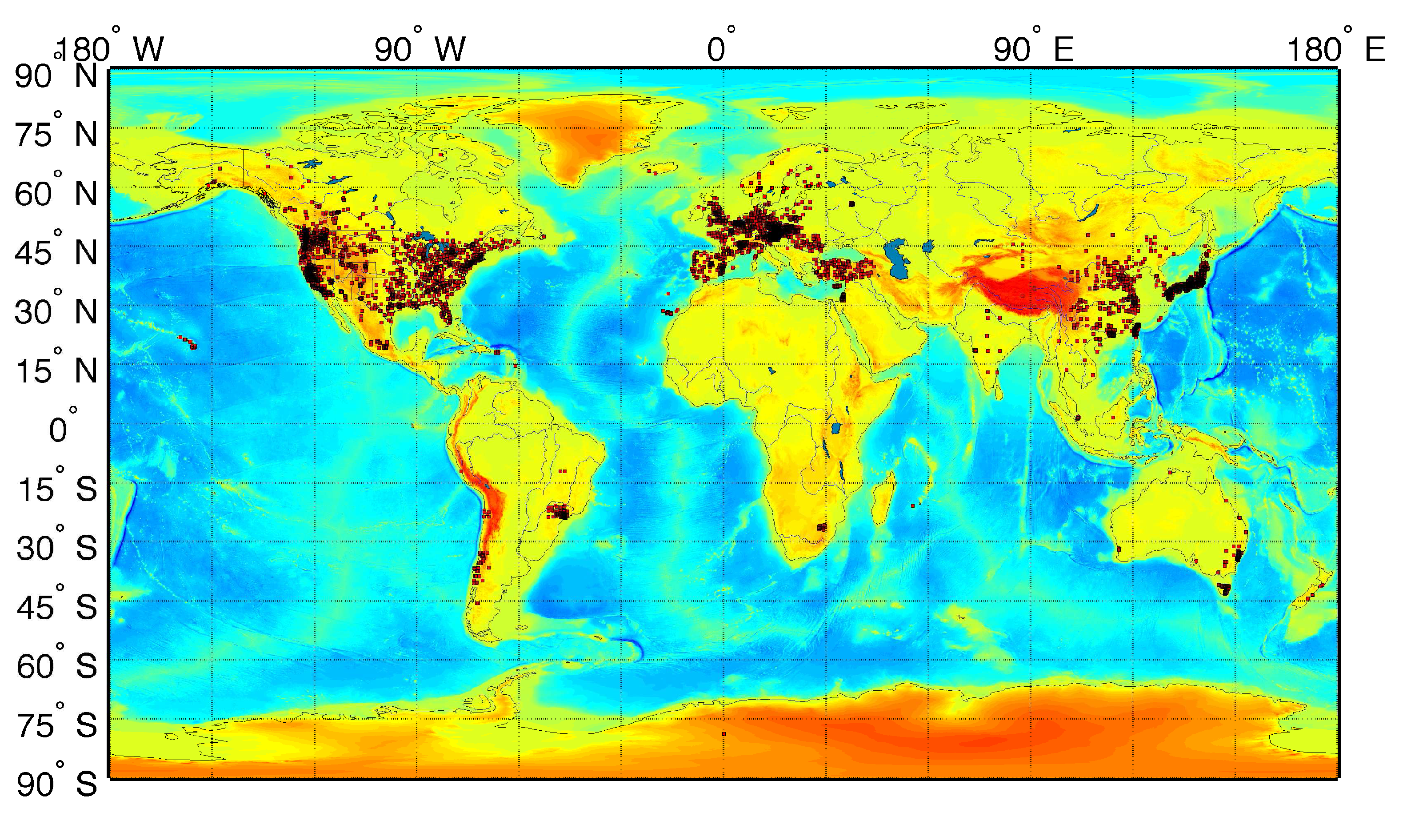
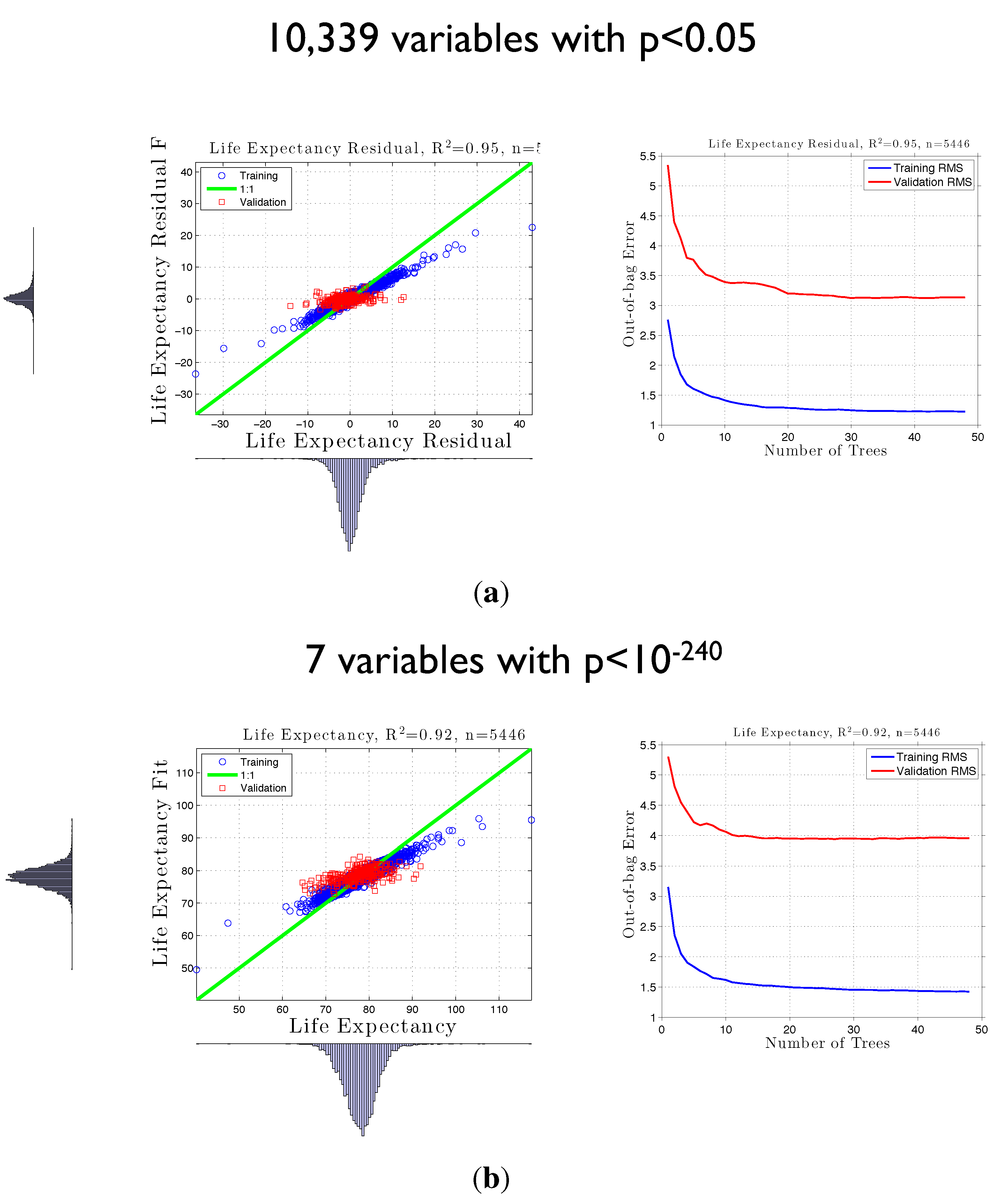
3.2. Life Expectancy and Socioeconomic Data from the U.S. Census

In 2012, the Center on Society and Health at Virginia Commonwealth University launched a two-year study of factors that affect life expectancy in California census tracts with high poverty rates. They calculated the life expectancy of thousands of census tracts in California, working with vital statistics supplied by the California Department of Health. The researchers were using traditional statistical techniques, such as regression equations, to study factors in these census tracts that might affect life expectancy, such as healthcare and public health, the physical and social environment, socioeconomic conditions of individuals and households and macrostructural resources. Their goal was to see if these factors seem to differ in outlier census tracts with unexpectedly high or low life expectancy given their poverty rate. The goal is to help elected officials and other policymakers identify assets that act positively to help poor communities buffer the adverse health effects of poverty. The parsimony required for traditional methods, as discussed above, required the researchers to handpicked a limited number of variables in each domain to enter into their regression equation.

Figure 3. The monthly average of our prototype machine learning PM_2.5 product (µg/m³) for August 2001. The average of the observations at a given site is overlaid as color-filled circles when observations were available for at least a third of the days. Notice the good agreement between the PM_2.5 product and the observations. Furthermore, as would be expected, in summer, the eastern U.S. has much higher PM_2.5 concentration than the western U.S. (a) Alaska highlighting common fire areas associated with elevated PM_2.5; (b,c) the good agreement between our product and the observations; (d) the elevated PM_2.5 with the heavily agricultural Central Valley in California, the highly populated Los Angeles Metro Area, the Sonoran Desert, one of the most active dust source regions in the U.S., the Four Corners Power Plants, some of the largest coal-fired generating stations in the U.S., and the Great Salt Lake Desert.

Figure 3. The monthly average of our prototype machine learning PM_2.5 product (µg/m³) for August 2001. The average of the observations at a given site is overlaid as color-filled circles when observations were available for at least a third of the days. Notice the good agreement between the PM_2.5 product and the observations. Furthermore, as would be expected, in summer, the eastern U.S. has much higher PM_2.5 concentration than the western U.S. (a) Alaska highlighting common fire areas associated with elevated PM_2.5; (b,c) the good agreement between our product and the observations; (d) the elevated PM_2.5 with the heavily agricultural Central Valley in California, the highly populated Los Angeles Metro Area, the Sonoran Desert, one of the most active dust source regions in the U.S., the Four Corners Power Plants, some of the largest coal-fired generating stations in the U.S., and the Great Salt Lake Desert.

Building on this study, we conducted a parallel project to serve as a demonstration of the power of machine learning. As a proof of concept, it was intentionally limited to one geographic area (the State of California) and one domain in the researchers’ model: socioeconomic conditions in individuals and households.

The 2007–2011 U.S. Census Bureau’s American Community Survey provides a rich data set on socioeconomic conditions for individuals and households that are too extensive for traditional researchers to examine in total, but that are arrayed at the census tract level in a downloadable form that supercomputers can easily analyze. The total number of variables available at the census tract level is extensive: a total of 21,038 variables spread across 113 data files. Some of the variables are duplicated in more than one file, and when these duplicates are removed, 18,528 unique variables remain. Some of these variables have missing values for certain census tracts; if variables with missing values are removed, then 13,065 variables remain. Although this is a staggering number of variables that most conventional investigators would not even attempt to analyze, we easily used machine learning to design a fully non-linear, non-parametric, multi-variate fit of all 13,065 variables. We calculated the bivariate statistical significance of the individual correlation of these variables with life expectancy and found that a staggering 10,339 variables had a p-value less than 0.05. The variables in the census are not orthogonal, and aspects of the same information content are duplicated in many census variables. If the p-value threshold is progressively decreased, we find that, remarkably, seven variables have a p-value of less than 10⁻²⁴⁰.

Whether we use all 13,065 variables or the 10,339 with a p-value of less than 0.05, or just the seven variables with a p-value of less than 10⁻²⁴⁰, machine learning is able to do a good job of estimating life expectancy. Two examples of the fully non-linear, non-parametric, multi-variate estimates of life expectancy using Random Forests [57,58] are shown in Figure 4.

A few obvious take away messages were found.

First, the variables that machine learning highlighted as most important replicated classic epidemiological studies in highlighting the importance of factors with known associations with life expectancy—age, sex, race-ethnicity, income/poverty, and education—however, in addition, the machine learning approach identified some additional key factors. Among the top 50, it identified other factors that ranked very highly in importance, including: relocation (first); employment, especially in certain industries (third, seventh, eighth, 13th, 15th, 19th, 20th, 36th, 42th, 49th); occupied housing (sixth, 11th, 16th, 18th, 21st, 31st, 50th); single-parent households (sixth, 12th); language (14th); grandparents living with grandchildren (26th, 48th); and SNAP eligibility (38th). Whether these variables are proxies for socioeconomic status or reflect unique influences on life expectancy independent of classic social determinants of health requires further analysis beyond the scope of this project.

Second, perhaps because key information in the census is duplicated many times, the fit using just seven variables was almost as good as that using all 13,065 variables, or the 10,339 with a p-value of less than 0.05.

Third, as good as the machine learning fit was, the slope of the scatter diagram is not exactly one. This data signature indicates that additional key factors have not been considered. This is not unexpected; this study focused only on the socioeconomic dimension and not other determinants of health, such as environmental factors, like air quality, or dietary habits and access to health care. It is clear that important factors related to life expectancy that need to be simultaneously accounted for are healthcare, health behaviors, the social environment, the physical environment (including pollution) and public spending on social and health services.

Figure 4. Two examples of the scatter diagrams for fully non-linear, non-parametric, multi-variate estimates of life expectancy: (a) 10,339 variables in the American Community Survey (U.S. Census Bureau) with a bivariate p-value for life expectancy of less than 0.05; (b) seven variables in the American Community Survey (U.S. Census Bureau) with a bivariate p-value for life expectancy of less than 10⁻²⁴⁰. Blue circles depict the training data. Red squares depict randomly selected, totally independent validation data not used in the training. The green line is the ideal 1:1 line for a perfect fit.

Figure 4. Two examples of the scatter diagrams for fully non-linear, non-parametric, multi-variate estimates of life expectancy: (a) 10,339 variables in the American Community Survey (U.S. Census Bureau) with a bivariate p-value for life expectancy of less than 0.05; (b) seven variables in the American Community Survey (U.S. Census Bureau) with a bivariate p-value for life expectancy of less than 10⁻²⁴⁰. Blue circles depict the training data. Red squares depict randomly selected, totally independent validation data not used in the training. The green line is the ideal 1:1 line for a perfect fit.

Therefore, we have seen that machine learning is a powerful tool for dealing with massively multi-variate systems, for letting the data speak, for highlighting key drivers and for providing objective tools that tell us when additional factors need to be considered.

3.3. False Positives

It is critical to recognize that correlation is not causation; further, when using machine learning with many variables, there is always the possibility of false associations. The full analysis of such possibilities are beyond the scope of this paper. However, one way to address these questions is some kind of experimental control in the data mining exercise, but a variety of other methods have been proposed.

4. Summary

Human health is part of an interdependent, multifaceted system, with many aspects varying geospatialy. The Holistics 3.0 paradigm that brings together data on as many aspects of a problem as possible and combines it with machine learning (and where necessary, causality) is a powerful tool for informing data-driven decisions that can incorporate and account for geospatial variations. Key in this is allowing the data to “speak for itself” and the ability to process thousands of variables simultaneously in a fully multi-variate, non-linear, non-parametric, non-Gaussian framework.

References

1. Jacobs, A. The pathologies of big data. Commun. ACM 2009, 52, 36–44. [Google Scholar] [CrossRef]
2. Guhaniyogi, R.; Finley, A.O.; Banerjee, S.; Gelfand, A.E. Adaptive Gaussian predictive process models for large spatial datasets. Environmetrics 2011, 22, 997–1007. [Google Scholar] [CrossRef] [PubMed]
3. Finley, A.O.; Banerjee, S.; Gelfand, A.E. Bayesian dynamic modeling for large space-time datasets using Gaussian predictive processes. J. Geogr. Syst. 2012, 14, 29–47. [Google Scholar] [CrossRef]
4. European Space Agency (ESA). Big Data from Space; European Space Agency: Frascati, Italy, 2013. [Google Scholar]
5. Hay, S.; George, D.; Moyes, C.; Brownstein, J. Big data opportunities for global infectious disease surveillance. PLoS Med. 2013, 10, e1001413. [Google Scholar] [CrossRef] [PubMed]
6. Karimi, H.A. (Ed.) Big Data: Techniques and Technologies in Geoinformatics; CRC Press: Boca Raton, FL, USA, 2014; p. 312.
7. Barton, D.; Court, D. Making advanced analytics work for you. Harv. Bus. Rev. 2012, 90, 78–83. [Google Scholar] [PubMed]
8. Davenport, T.; Patil, D. Data Scientist: The Sexiest Job of the 21st Century. Harvard Business Review, Ocotber 2012. [Google Scholar]
9. McAfee, A.; Brynjolfsson, E. Big Data: The Management Revolution. Harvard Business Review, October 2012. [Google Scholar]
10. Murdoch, T.; Detsky, A. The inevitable application of big data to health care. JAMA 2013, 309, 1351–1352. [Google Scholar] [CrossRef] [PubMed]
11. Pearl, J. Causality: Models, Reasoning and Inference; Cambridge University Press: New York, NY, USA, 2009. [Google Scholar]
12. Noble, D.; Casalino, L. Can accountable care organizations improve population health? Should they try? JAMA 2013, 11, 119–120. [Google Scholar]
13. Ruckerl, R.; Schneider, A.; Breitner, S.; Cyrys, J.; Peters, A. Health effects of particulate air pollution: A review of epidemiological evidence. Inhalation Toxicol. 2011, 23, 555–592. [Google Scholar] [CrossRef]
14. Engel-Cox, J.A.; Hoff, R.M.; Haymet, A.D.J. Recommendations on the use of satellite remote-sensing data for urban air quality. J. Air Waste Manag. Assoc. 2004, 54, 1360–1371. [Google Scholar] [CrossRef] [PubMed]
15. Engel-Cox, J.A.; Holloman, C.H.; Coutant, B.W.; Hoff, R.M. Qualitative and quantitative evaluation of MODIS satellite sensor data for regional and urban scale air quality. Atmos. Environ. 2004, 38, 2495–2509. [Google Scholar] [CrossRef]
16. Engel-Cox, J.A.; Hoff, R.M.; Rogers, R.; Dimmick, F.; Rush, A.C.; Szykman, J.J.; Al-Saadi, J.; Chu, D.A.; Zell, E.R. Integrating lidar and satellite optical depth with ambient monitoring for 3-dimensional particulate characterization. Atmos. Environ. 2006, 40, 8056–8067. [Google Scholar] [CrossRef]
17. Liu, Y.; Sarnat, J.A.; Kilaru, A.; Jacob, D.J.; Koutrakis, P. Estimating ground-level PM2.5 in the Eastern United States using satellite remote sensing. Environ. Sci. Technol. 2005, 39, 3269–3278. [Google Scholar] [CrossRef] [PubMed]
18. Liu, Y.; Franklin, M.; Kahn, R.; Koutrakis, P. Using aerosol optical thickness to predict ground-level PM2.5 concentrations in the St. Louis area: A comparison between MISR and MODIS. Remote Sens. Environ. 2007, 107, 33–44. [Google Scholar] [CrossRef]
19. Liu, Y.; Paciorek, C.; Koutrakis, P. Estimating daily PM2.5 exposure in Massachusetts with satellite aerosol remote sensing data, meteorological, and land use information. Epidemiology 2008, 19, S116. [Google Scholar]
20. Van Donkelaar, A.; Martin, R.V.; Park, R.J. Estimating ground-level PM2.5 using aerosol optical depth determined from satellite remote sensing. J. Geophys. Res. 2006, 111. [Google Scholar] [CrossRef]
21. Van Donkelaar, A.; Martin, R.; Verduzco, C.; Brauer, M.; Kahn, R.; Levy, R.; Villeneuve, P. A hybrid approach for predicting PM2.5 exposure response. Environ. Health Perspect. 2010, 118. [Google Scholar] [CrossRef]
22. Van Donkelaar, A.; Martin, R.V.; Brauer, M.; Kahn, R.; Levy, R.; Verduzco, C.; Villeneuve, P.J. Global estimates of ambient fine particulate matter concentrations from satellite-based aerosol optical depth: Development and application. Environ. Health Perspect. 2010, 118, 847–855. [Google Scholar] [CrossRef] [PubMed]
23. Van Donkelaar, A.; Martin, R.V.; Levy, R.C.; da Silva, A.M.; Krzyzanowski, M.; Chubarova, N.E.; Semutnikova, E.; Cohen, A.J. Satellite-based estimates of ground-level fine particulate matter during extreme events: A case study of the Moscow fires in 2010. Atmos. Environ. 2011, 45, 6225–6232. [Google Scholar] [CrossRef]
24. Martin, R.V. Satellite remote sensing of surface air quality. Atmos. Environ. 2008, 42, 7823–7843. [Google Scholar] [CrossRef]
25. Hoff, R.M.; Christopher, S.A. Remote sensing of particulate pollution from space: Have we reached the promised land? J. Air Waste Manag. Assoc. 2009, 59, 645–675. [Google Scholar] [CrossRef] [PubMed]
26. Hoffmann, B.; Moebus, S.; Dragano, N.; Stang, A.; Moehlenkamp, S.; Schmermund, A.; Memmesheimer, M.; Broecker-Preuss, M.; Mann, K.; Erbel, R.; et al. Chronic residential exposure to particulate matter air pollution and systemic inflammatory markers. Environ. Health Perspect. 2009, 117, 1302–1308. [Google Scholar] [CrossRef] [PubMed]
27. Zhang, H.; Hoff, R.M.; Engel-Cox, J.A. The relation between Moderate Resolution Imaging Spectroradiometer (MODIS) aerosol optical depth and PM2.5 over the United States: A geographical comparison by US Environmental Protection Agency Regions. J. Air Waste Manag. Assoc. 2009, 59, 1358–1369. [Google Scholar] [CrossRef] [PubMed]
28. Zhang, H.; Lyapustin, A.; Wang, Y.; Kondragunta, S.; Laszlo, I.; Ciren, P.; Hoff, R.M. A multi-angle aerosol optical depth retrieval algorithm for geostationary satellite data over the United States. Atmos. Chem. Phys. 2011, 11, 11977–11991. [Google Scholar] [CrossRef]
29. Weber, S.A.; Engel-Cox, J.A.; Hoff, R.M.; Prados, A.I.; Zhang, H. An improved method for estimating surface fine particle concentrations using seasonally adjusted satellite aerosol optical depth. J. Air Waste Manag. Assoc. 2010, 60, 574–585. [Google Scholar] [CrossRef] [PubMed]
30. Kumar, N.; Chu, A.D.; Foster, A.D.; Peters, T.; Willis, R. Satellite remote sensing for developing time and space resolved estimates of ambient particulate in Cleveland, OH. Aerosol Sci. Technol. 2011, 45, 1090–1108. [Google Scholar] [CrossRef] [PubMed]
31. Lee, H.J.; Liu, Y.; Coull, B.; Schwartz, J.; Koutrakis, P. PM2.5 prediction modeling using MODIS AOD and its implications for health effect studies. Epidemiology 2011, 22, S215. [Google Scholar] [CrossRef]
32. Lee, H.J.; Liu, Y.; Coull, B.A.; Schwartz, J.; Koutrakis, P. A novel calibration approach of MODIS AOD data to predict PM2.5 concentrations. Atmos. Chem. Phys. 2011, 11, 7991–8002. [Google Scholar] [CrossRef]
33. Choi, Y.S.; Ho, C.H.; Chen, D.; Noh, Y.H.; Song, C.K. Spectral analysis of weekly variation in PM10 mass concentration and meteorological conditions over China. Atmos. Environ. 2008, 42, 655–666. [Google Scholar] [CrossRef]
34. Liu, Y.; Koutrakis, P.; Kahn, R. Estimating fine particulate matter component concentrations and size distributions using satellite-retrieved fractional aerosol optical depth: Part 1—Method development. J. Air Waste Manag. Assoc. 2007, 57, 1360–1369. [Google Scholar] [CrossRef] [PubMed]
35. Liu, Y.; Koutrakis, P.; Kahn, R.; Turquety, S.; Yantosca, R.M. Estimating fine particulate matter component concentrations and size distributions using satellite-retrieved fractional aerosol optical depth: Part 2—A case study. J. Air Waste Manag. Assoc. 2007, 57, 1360–1369. [Google Scholar] [CrossRef] [PubMed]
36. Liu, Y.; Paciorek, C.J.; Koutrakis, P. Estimating regional spatial and temporal variability of PM2.5 concentrations using satellite data, meteorology, and land use information. Environ. Health Perspect. 2009, 117, 886–892. [Google Scholar] [CrossRef] [PubMed]
37. Liu, Y.; Chen, D.; Kahn, R.A.; He, K. Review of the applications of multiangle imaging spectroradiometer to air quality research. Sci. China Ser. D-Earth Sci. 2009, 52, 132–144. [Google Scholar] [CrossRef]
38. Liu, Y.; Kahn, R.A.; Chaloulakou, A.; Koutrakis, P. Analysis of the impact of the forest fires in August 2007 on air quality of Athens using multi-sensor aerosol remote sensing data, meteorology and surface observations. Atmos. Environ. 2009, 43, 3310–3318. [Google Scholar] [CrossRef]
39. Liu, Y.J.; Harrison, R.M. Properties of coarse particles in the atmosphere of the United Kingdom. Atmos. Environ. 2011, 45, 3267–3276. [Google Scholar] [CrossRef]
40. Liu, Y.; He, K.; Li, S.; Wang, Z.; Christiani, D.C.; Koutrakis, P. A statistical model to evaluate the effectiveness of PM2.5 emissions control during the Beijing 2008 Olympic Games. Environ. Int. 2012, 44, 100–105. [Google Scholar] [CrossRef] [PubMed]
41. Lyamani, H.; Olmo, F.J.; Alcantara, A.; Alados-Arboledas, L. Atmospheric aerosols during the 2003 Heat Wave in southeastern Spain I: Spectral optical depth. Atmos. Environ. 2006, 40, 6453–6464. [Google Scholar] [CrossRef]
42. Pelletier, B.; Santer, R.; Vidot, J. Retrieving of particulate matter from optical measurements: A semiparametric approach. J. Geophys. Res.-Atmos. 2007, 112. [Google Scholar] [CrossRef]
43. Wang, Q.; Shao, M.; Liu, Y.; William, K.; Paul, G.; Li, X.; Liu, Y.; Lu, S. Impact of biomass burning on urban air quality wstimated by organic tracers: Guangzhou and Beijing as cases. Atmos. Environ. 2007, 41, 8380–8390. [Google Scholar] [CrossRef]
44. Natunen, A.; Arola, A.; Mielonen, T.; Huttunen, J.; Komppula, M.; Lehtinen, K.E.J. A multi-year comparison of PM2.5 and AOD for the Helsinki region. Boreal Environ. Res. 2010, 15, 544–552. [Google Scholar]
45. Paciorek, C.J.; Liu, Y.; Moreno-Macias, H.; Kondragunta, S. Spatiotemporal associations between GOES aerosol optical depth retrievals and ground-level PM2.5. Environ. Sci. Technol. 2008, 42, 5800–5806. [Google Scholar] [CrossRef] [PubMed]
46. Paciorek, C.J.; Liu, Y. Limitations of remotely sensed aerosol as a spatial proxy for fine particulate Matter. Environ. Health Perspect. 2009, 117. [Google Scholar] [CrossRef]
47. Paciorek, C.J.; Liu, Y. Assessment and Statistical Modeling of the Relationship between Remotely Sensed Aerosol Optical Depth and PM2.5 in the Eastern United States; Research Report; Health Effects Institute: Boston, MA, USA, 2012. [Google Scholar]
48. Rajeev, K.; Parameswaran, K.; Nair, S.K.; Meenu, S. Observational evidence for the radiative impact of Indonesian smoke in modulating the sea surface temperature of the equatorial Indian Ocean. J. Geophys. Res.-Atmos. 2008, 113. [Google Scholar] [CrossRef]
49. Schaap, M.; Apituley, A.; Timmermans, R.M.A.; Koelemeijer, R.B.A.; de Leeuw, G. Exploring the relation between aerosol optical depth and PM2.5 at Cabauw, The Netherlands. Atmos. Chem. Phys. 2009, 9, 909–925. [Google Scholar] [CrossRef]
50. Tian, D.; Wang, Y.; Bergin, M.; Hu, Y.; Liu, Y.; Russell, A.G. Air quality impacts from prescribed forest fires under different management practices. Environ. Sci. Technol. 2008, 42, 2767–2772. [Google Scholar] [CrossRef] [PubMed]
51. Van de Kassteele, J.; Koelemeijer, R.B.A.; Dekkers, A.L.M.; Schaap, M.; Homan, C.D.; Stein, A. Statistical mapping of PM10 concentrations over western Europe using secondary information from dispersion modeling and MODIS satellite observations. Stoch. Environ. Res. Risk Assess. 2006, 21, 183–194. [Google Scholar] [CrossRef]
52. Zhang, J.; Reid, J.S. An analysis of clear sky and contextual biases using an operational over ocean MODIS aerosol product. Geophys. Res. Lett. 2009, 36. [Google Scholar] [CrossRef]
53. Lary, D.J.; Remer, L.A.; MacNeill, D.; Roscoe, B.; Paradise, S. Machine learning and bias correction of MODIS aerosol optical depth. IEEE Geosci. Remote Sens. Lett. 2009, 6, 694–698. [Google Scholar] [CrossRef]
54. Hyer, E.J.; Reid, J.S.; Zhang, J. An over-land aerosol optical depth data set for data assimilation by filtering, correction, and aggregation of MODIS Collection 5 optical depth retrievals. Atmos. Meas. Tech. 2011, 4, 379–408. [Google Scholar] [CrossRef]
55. Shi, Y.; Zhang, J.; Reid, J.S.; Hyer, E.J.; Hsu, N.C. Critical evaluation of the MODIS Deep Blue aerosol optical depth product for data assimilation over North Africa. Atmos. Meas. Tech. Discuss. 2012, 5, 7815–7865. [Google Scholar] [CrossRef]
56. Reid, J.S.; Hyer, E.J.; Johnson, R.S.; Holben, B.N.; Yokelson, R.J.; Zhang, J.; Campbell, J.R.; Christopher, S.A.; Girolamo, L.D.; Giglio, L.; et al. Observing and understanding the Southeast Asian aerosol system by remote sensing: An initial review and analysis for the Seven Southeast Asian Studies (7SEAS) program. Atmos. Res. 2013, 122, 403–468. [Google Scholar] [CrossRef]
57. Ho, T.K. The random subspace method for constructing decision forests. IEEE Trans. Pattern Anal. Mach. Intell. 1998, 20, 832–844. [Google Scholar] [CrossRef]
58. Breiman, L. Random forests. Mach. Learn. 2001, 45, 5–32. [Google Scholar] [CrossRef]