GIS-Based Analytical Tools for Transport Planning: Spatial Regression Models for Transportation Demand Forecast

Abstract

Considering the importance of spatial issues in transport planning, the main objective of this study was to analyze the results obtained from different approaches of spatial regression models. In the case of spatial autocorrelation, spatial dependence patterns should be incorporated in the models, since that dependence may affect the predictive power of these models. The results obtained with the spatial regression models were also compared with the results of a multiple linear regression model that is typically used in trips generation estimations. The findings support the hypothesis that the inclusion of spatial effects in regression models is important, since the best results were obtained with alternative models (spatial regression models or the ones with spatial variables included). This was observed in a case study carried out in the city of Porto Alegre, in the state of Rio Grande do Sul, Brazil, in the stages of specification and calibration of the models, with two distinct datasets.

1. Introduction

Spatial relationships play an important role in transport. Even though, there are not so many studies focusing on the explicit introduction of spatial issues in transport planning modeling. Thus, as a contribution to the field, the objective of this study is to analyze the results obtained from different approaches of spatial regression models. Next, the outcomes of these spatial models are also compared with the results of a multiple linear regression model that is typically used in trips generation estimations. The key research question of this study was thus whether or not the inclusion of spatial variables improves transport demand models. Many researchers have already discussed the importance of considering spatial effects in urban and transportation analyses. Páez and Scott [1], for instance, have made a review of techniques and examples of applications illustrating how spatial statistics can be used in urban transportation and land use planning. The objective of that study was to discuss some of the major technical issues in spatial analysis (i.e., spatial association, heterogeneity and the modifiable areal unit problem) and the authors indicated a promising trend for the application of increasingly sophisticated spatial statistical methods in urban analyses. These topics are still timely, as recently discussed by Wang et al. [2].

Spatial dependence and its effects on transportation demand models, which are the focus of this study, are undoubtedly among the issues concerning spatial analysis that have not been fully explored in transport planning yet. This can be seen in Table 1, in which a review of studies conducted in the past three decades about spatial effects on transportation and urban analysis was summarized. The table is organized in such a way that the references are shown in the central column, the spatial analytical issues explored are listed on the left side of the table and the fields of application are listed on the right side of the table. Regarding the spatial analytical issues, most of the selected studies focused on issues of spatial association (i.e., spatial dependence or spatial autocorrelation). Regarding the applications, only a few of them dealt with transportation demand analyses. It is worth mentioning that almost all studies have reached a common conclusion: the inclusion of spatial effects improved the analyses results. This is not really a surprise, but it calls the attention to the fact that many studies that are not listed in Table 1 still do not explicitly include spatial analysis elements in their analyses.

Regression models, for example, are commonly used in the trip generation phase of transport planning. They are statistical tools that explore the existing relationships among two or more variables, so that one of them can be explained (and therefore its value can be estimated) by the other(s). However, in the presence of a significant spatial autocorrelation, model estimations have to consider and to incorporate the spatial structure of data. Spatial regressions, or regression analyses incorporating the existing spatial dependence of data, are likely to improve the predictive power of the regression models.

Bolduc et al. [3,4,5], Haider and Miller [6], Wang [7], Czado and Prokopenko [8], Kawamura and Mahajan [9], Vichiensan et al. [10], Zhou and Kockelman [11], Ribeiro and Antunes [12], Chalermpong [13], Hackney et al. [14,15], and Novak et al. [16] provide examples of applications of spatial regression, some of them in urban and transportation planning. In general, the spatial models tested had a better fit to the actual data than the respective non-spatial models.

Table 1. Applications of spatial statistics in transport analysis.

Spatial Analytical Issues Explored			Studies Reviewed	Fields Of Application
Spatial Association (Spatial Dependence)	Spatial Heterogeneity	Modifiable Areal Unit Problem (MAUP)		Travel Demand Estimations	Travel Behavior	Transportation-Land Use Modeling and Data Estimation
	X		Bender and Hwang [17]			X
X			Bolduc et al. [3], Eom et al. [18], Wang and Kockelman [19]	X
X	X		Bolduc et al. [4,5], Bhat and Zhao [20], Czado and Prokopenko [8]	X
X			Kwan [21], Steenberghen et al. [22], Li and Zhang [23], Hackney et al. [14], Hackney et al. [15], Gundogdu et al. [24], Khan et al. [25], Guo et al. [26], Páez et al. [27]		X
X			Haider and Miller [6], Wang [7], Kawamura and Mahajan [9], Victoria et al. [28], Chalermpong [13], Zhou and Kockelman [11], Ibeas et al. [29], Efthymiou and Antoniou [30]			X
		X	Horner and Murray [31]			X
X	X		Vichiensan et al. [10], Ribeiro and Antunes [12]			X
X			Novak et al. [16]

Table 1. Applications of spatial statistics in transport analysis.

Spatial Analytical Issues Explored			Studies Reviewed	Fields Of Application
Spatial Association (Spatial Dependence)	Spatial Heterogeneity	Modifiable Areal Unit Problem (MAUP)		Travel Demand Estimations	Travel Behavior	Transportation-Land Use Modeling and Data Estimation
	X		Bender and Hwang [17]			X
X			Bolduc et al. [3], Eom et al. [18], Wang and Kockelman [19]	X
X	X		Bolduc et al. [4,5], Bhat and Zhao [20], Czado and Prokopenko [8]	X
X			Kwan [21], Steenberghen et al. [22], Li and Zhang [23], Hackney et al. [14], Hackney et al. [15], Gundogdu et al. [24], Khan et al. [25], Guo et al. [26], Páez et al. [27]		X
X			Haider and Miller [6], Wang [7], Kawamura and Mahajan [9], Victoria et al. [28], Chalermpong [13], Zhou and Kockelman [11], Ibeas et al. [29], Efthymiou and Antoniou [30]			X
		X	Horner and Murray [31]			X
X	X		Vichiensan et al. [10], Ribeiro and Antunes [12]			X
X			Novak et al. [16]

This study focus on the results of the trip generation phase of the four-step model (i.e., trip generation, trip distribution, transport mode choice and route choice). Thus, it aims to contribute to the evaluation of the benefits in the application of spatial statistics tools in the analysis of demand for transport and for sustainable transport planning.

Lopes and Rodrigues da Silva [32] assessed the impacts of the introduction of global and local indicators of spatial dependence in demand forecast models. Models with spatial characteristics, which were called “alternative” models, were compared with “traditional” models, in which the variables were not treated in spatial terms. The method was applied in the city of Porto Alegre, which is the capital of the state of Rio Grande do Sul, Brazil. The data for the analyses came from origin-destination (O-D) surveys obtained through household interviews (hereafter called EDOM, which is the acronym for household interviews in Portuguese) in two distinct years (1974 and 1986). The 1974 dataset was used for calibration and adjustment of the models. The 1986 dataset provided the information needed for analyzing the estimates based on the 1974 models. Several models were tested and the most efficient one was that in which Global and Local spatial variables were introduced. These years were selected because these are the datasets available in the city of Porto Alegre.

In this study, we further developed our own previous studies by analyzing the results obtained with the model that was best adjusted to the 1974 dataset. The so-called AGL74 model, which stands for Alternative, Global and Local model for the year 1974, was a multiple regression model that received the “alternative” designation because of the spatial variables that represented indicators of global and local spatial dependence. In addition to the model AGL74, we used the same datasets from Porto Alegre to analyze the results of the following alternative regression models that consider global spatial effects: the Spatial Auto-Regressive Model and the Spatial Error Model (Anselin [33] and Fotheringham et al. [34]).

The performance of the models was also tested with data of a more recent origin-destination survey in the phases of validation and forecast. Those data, which were obtained through household interviews in 2003 (EDOM, 2003), were not available when the previous studies were conducted. Thus, in this article we presented the results obtained with the implementation of the alternative models calibrated with the 1974 and 2003 datasets. In addition, we carried out comparative analyses with the results of traditional models that were also calibrated with the same datasets.

Two topics that are relevant to this study were discussed in a brief literature review right after this introduction. Initially, Exploratory Spatial Data Analysis (ESDA, as described by Anselin [35]) tools were discussed in Section 2. Those tools served to generate the indicators that were introduced as spatial variables in the alternative models. They were also essential in the analysis of the models results. Next, Confirmatory Spatial Data Analysis (CSDA) tools were also treated in Section 2. We focused specifically on Spatial Regression, as follows: first we have provided an overview of the subject and we subsequently presented the structure of the models we have selected for use. In Section 3, we presented details of the methodology used in the study, followed by an analysis of the results of our application in Section 4, and the main conclusions of the study in Section 5.

2. Exploratory and Confirmatory Spatial Data Analysis Tools

Exploratory Spatial Data Analysis (ESDA) tools can be used to: (i) visualize and describe spatial distributions; (ii) identify standards of spatial association (spatial agglomerations or clusters); (iii) identify atypical observations (extreme values or outliers); and (iv) identify the existence of spatial instabilities (non-stationarity). ESDA methods are descriptive and not confirmatory. Therefore, they are not meant to be used to patterns detection, hypotheses elaboration, and estimation of spatial models (Anselin [35]).

Spatial autocorrelation is among the analyses conducted with ESDA tools. A value of spatial autocorrelation can show how much the value of a variable in one region is dependent on the values of the same variable in neighborhood locations. For example, the Moran’s I Index indicates, through values that vary from −1 to +1, how similar each area is to its immediate neighbor in relation to a particular variable. While zero means no spatial autocorrelation, values close to −1 or +1 indicate the presence of negative or positive autocorrelation, respectively. As a result, by allowing the identification of nonrandom distributions of the variables, Moran’s I can be useful in the analyses at the initial stages of transport modeling, when regression equations are extensively used in the four-step model.

The Moran Scatterplot can be used to obtain global spatial variables (or global indicators of spatial dependence). It is a two-dimensional graph divided into four quadrants, in which normalized values of the analysis variable (Z) are compared with the average of the values in neighboring zones (W_z). The Moran’s I value is equivalent to the coefficient that indicates the slope (α) of a regression line of W_z in Z. The quadrants can be interpreted as proposed by Anselin [36]:

• Q1 (positive value for the zone and positive value for the average of the values in neighboring zones) and Q2 (negative value for the zone and negative value for the average of the values in neighboring zones). It indicates points of positive spatial association, what means that a zone has neighbor zones with similar values. Also called High-High and Low-Low, respectively.
• Q3 (negative value for the zone and positive value for the average of the values in neighboring zones) and Q4 (positive value for the zone and negative value for the average of the values in neighboring zones). It indicates points of negative spatial association, what means that a zone has distinct values from its neighbors. Also called Low-High and High-Low, respectively.

Moran’s Scatterplot values can also be presented in the so-called Box Maps. In such a map, each polygon is classified according to the quadrant it belongs to in the scatter diagram. While the global indicators, like Moran’s I, provide a unique value as a measure of data spatial association, the local indicators produce a specific value for each area. They allow the identification of regions with: similar attribute values (clusters), outliers, and more than a spatial regime. Anselin [35] refers to them as LISA (Local Indicators of Spatial Association) statistics.

The statistical significance of Moran’s local indicators can be computed as follows. The process starts with the calculation of the indexes for each area. The values of all areas are then randomly permuted until a pseudo distribution is obtained, for which significant parameters can be calculated. In this case, the LISA Map and the Moran Map indicate the regions that present local correlation significantly different from the rest of the data. They are areas with their own spatial dynamics (i.e., pockets of local non-stationarity) that require detailed analysis. Significant autocorrelations to a level of 5% indicate very similar areas in comparison to their neighbors.

The spatial variables were introduced into the transport demand models in the present study through Local Moran statistics. They were obtained as local indicators of spatial dependence and denominated local spatial variables. The ESDA indices and tools were also very useful in the evaluation of the models performance, since they can be used in the analysis of the spatial distribution of the estimation errors.

Confirmatory Spatial Data Analysis (CSDA) tools group the quantitative processes of modeling, estimation and validation necessary for the analysis of spatial components. It can be highlighted, in this group, the “toolkit” available for spatial statistics and spatial econometrics as spatial regression, or the introduction of indicators of spatial autocorrelation as spatial variables in regression models.

Typically, when performing regression analysis, the aim is to find a good fit between predicted and observed values of the dependent variable in the model. In addition, it is important to find which of the variables significantly contribute to the linear relationship. The standard hypothesis is that the observations are not correlated and, as such, the residuals ε_i of the model, which follow a Normal Distribution with a zero average and constant variance, are independent and uncorrelated to the dependent variable. However, in the case of data that are spatially dependent, it is very unlikely that the standard hypothesis of uncorrelated observations is true. In the most common case, the residues continue to display spatial autocorrelation in the data that can be manifested in systematic regional differences, or even through a continuous spatial trend.

Regression analyses of spatial data improve the predictive power of a model by incorporating the spatial dependence between data into the model. Initially, an exploratory analysis must be conducted with the aim of identifying the structure of dependence in the data. This is very important for the definition on how to incorporate this dependence into the regression model. Two basic types of spatial regression allow the incorporation of the spatial effects: those of Global form and those of Local form (Anselin [33] and Fotheringham et al. [34]). The Global models capture the spatial structure through a unique parameter that is added to the traditional regression model. The simplest spatial regression models, formally presented by Anselin [33], are the Spatial Auto Regressive (SAR) or Spatial Lag Model and the Conditional Auto Regressive (CAR) or Spatial Error Model.

2.1. SAR (Spatial Auto Regressive)

In the model SAR (or LAG, as it is called in this study) the ignored spatial autocorrelation is attributed to the Y variable. The spatial dependence is incorporated into the linear regression model by the addition of a new term in the form of a spatial relationship to the dependent variable. Formally, Anselin [33] introduced the model SAR by Equation (1). The null hypothesis for non-existence of autocorrelation is that ρ = 0. The basic idea is to incorporate spatial autocorrelation as a component of the model.

Y = ρWY + Xβ + ε

(1)

where: Y = dependent variable; X = independent variable; β = regression coefficients; ε = random errors with average zero and variance σ²; W = contiguity matrix or spatial weighted matrix; ρ = spatial autoregressive coefficient.

According to Getis and Griffith [37], these models depend on one or more spatial structural matrices that account for spatial autocorrelation in the georeferenced data from which model parameters are estimated. The same authors also mentioned that spatial autoregressive models almost exclusively assume normality, and are nonlinear in nature. In this way, for these models, it is inappropriate to use ordinary least squares (OLS) estimation procedures for model development and testing. Furthermore, these models provide global measures of spatial dependence, but they do not reveal individual spatial and nonspatial contributions of the components.

2.2. CAR (Conditional Auto Regressive)

In the second type of spatial regression model with global parameters, also referred to as Spatial Error Model, the spatial effects are considered as a noise, or disturbance, i.e., a factor that needs to be removed. In this case, the effects of spatial autocorrelation are associated with the error term ε and the model can be expressed by Equation (2). The null hypothesis for non-existence of autocorrelation is that λ = 0, i.e., the error term is not spatially correlated.

Y = Xβ + ε,  ε = λWε + ξ

(2)

where: Wε = errors with spatial effects; ξ = random errors with average zero and variance σ²; λ = autoregressive coefficient.

2.3. Models with Local and Global Indicators of Spatial Dependence

Another way to consider the spatial dependence in the regression models, which is called in the present study the alternative transport model, consists in the introduction of indicators of spatial autocorrelation (Global and Local) as variables. They are added to the traditional variables in the multiple regression model, or traditional model (as suggested by Lopes and Rodrigues da Silva [32]). In this way, the global and local spatial variables are defined and obtained through spatial analysis of the socioeconomic variables with the use of ESDA tools through spatial statistics computer packages.

The global spatial variables are binary (dummy) variables associated to the quadrants of the Moran Scatterplot (global indicator). For an independent variable “X”, three variables (X_Q1, X_Q2 and X_Q3) are defined to represent the spatial regime of each Traffic Analysis Zone (TAZ). For the definition of the local spatial variables (LISA_X), LISA indicators are considered. In the existence of spatial dependence influencing the results of the traditional models, Lopes and Rodrigues da Silva [32] showed that the alternative models were more efficient than the Global spatial regression models (SAR and CAR) in the prediction of home-based trip productions (HBTP) for the data of Porto Alegre.

Alternative models also require rigorous analyses of the significance of the included variables, in order to avoid the addition of unnecessary variables. A stepwise forward regression method was used, in addition to the tools available in the GIS-T software package, to analyze the changes produced in the models with the inclusion of spatial variables. The process is presented in detail in Section 4.3 and Section 4.8. Briefly stated, the method verifies if the addition of a new variable to the model causes a significant increase in the adjusted R-squared. The method does not exclude, however, the evaluation of model results by analysts, since in some cases the tools used may not be able to identify multicollinearity problems. However, the approach allows the use of traditional linear regression techniques while insuring that regression residuals behave according to required model assumptions, such as uncorrelated errors.

2.4. Evaluation of Spatial Models

A visual analysis of the residuals on a graph is an important step for assessing the adjustment of a regression. Mapping residuals is also useful, given that a high concentration of either positive or negative values in a part of the map is a good indicator of the presence of spatial autocorrelation. The Moran’s I index of residuals is commonly used as a quantitative test.

Maximum likelihood values weighted by the difference in the number of estimated parameters are commonly used to select regression models. In the models with a dependence structure (spatial or temporal), the evaluation of the adjustment is penalized by the number of parameters. Usually, the comparison of models uses the log-likelihood that represents the best adjustment to the observed data. The Akaike Information Criterion is expressed in Equation (3). The best model is the one that has the lowest AIC value. Many other information criteria are available in GIS packages with spatial statistics, through CSDA tools. Most of them are variations of AIC, with changes in the penalization of parameters or observations.

AIC = −2 × LIK + 2k

(3)

where: LIK = log-likelihood; k = number of regression coefficients.

3. Method

Most procedures were carried out in a GIS environment, with the additional use of the software package GeoDA [37], given it contains ESDA and CSDA tools (e.g., spatial regression modeling) that can be used for obtaining the spatial variables and for the calibration of the models.

The calibration and validation of the models was based on data of two origin and destination surveys conducted in the city of Porto Alegre, Brazil, in 1974 and 2003, as follows.

• “Base-year”—the 1974 dataset (EDOM 74) was used for the calibration and also for checking the performance of the best demand models. They could be either traditional or alternative models. While the former relied on traditional methods, the latter used variables that incorporate the degree of spatial dependence. In both cases, though, they were used to forecast transport demand.
• “Target-year”—as 2003 was taken as the forecast year, the EDOM 2003 dataset was used for comparison with the future trip estimations, which were obtained through the application of traditional and alternative models. The dataset contained information of the latest O-D survey and it was obtained through household interviews. That database, which was here used to measure the performance of the model, was not available for the previous studies of Lopes and Rodrigues da Silva [32].

The goodness-of-fit of the models was evaluated through statistical tests, such as the Adjusted R-Squared and AIC (Akaike Information Criterion), among others. The predictive power was evaluated by some measures of performance, such as MRE (mean relative error) and the Moran’s I for the errors. For the variables, the significance (t-Student), the presence of multicollinearity (multicollinearity condition number), and the condition of spatial autocorrelation were analyzed. Spatial autocorrelation values were also examined for the residuals. They were also tested to confirm the conditions of normal distribution and homoscedasticity.

The applied method can be summarized in four steps. First, the efficiency of the alternative models studied here was analyzed through a comparison of their results with those provided by the multiple regression model named T74. The T74 model best fits the 1974 data, but did not include any information about the spatial distribution of the data. The second step was to apply the best alternative model for estimating future trips. The 2003 O-D survey dataset provided the actual information for comparison with the estimations produced with the T74 model for the same year. In the third step, new models were calibrated for 2003 using the same structure of the models adjusted for 1974. Given the time span of nearly 30 years, changes in the relationships between variables would have been expected. Therefore, any variations in the coefficients of the variables were carefully analyzed. This phase was also meant to find which of the models tested for 1974 best fitted the data of 2003.

The last step was to find the most significant variables for 2003 and the model with the best adjustment to the actual data, based on the assumption that the introduction of spatial indicators would improve the model performance. A stepwise forward regression method was also used, in addition to the tools available in the GIS-T software package, to analyze the changes produced in the models with the inclusion of spatial variables.

It should be noted that the focus of the study was restricted to the stage of home-based trip productions (HBTP), which is just a part of the first step of the four-step model or urban transportation planning (UTP) procedure. Also, the trips were not separated by mode or purpose, because that information was not available in the base-year dataset. Hence, the proposed method does not intend to end the discussions on the subject. On the contrary, the idea is to foster research about the use of spatial analysis tools and techniques in transport planning, as suggested by Wang et al. [2].

4. Results and Discussion

The results are presented in this section in the same order that the models were built, starting with conventional variables and the 1974 dataset.

4.1. Multiple Regression-Traditional Model with the 1974 Dataset (T74)

The main outcomes of model T74, which was the multiple regression model initially adjusted to the 1974 dataset with the computer program GeoDA, are summarized in Table 2. The standardized values of population (POPst) and car fleet (CARst) were used as independent variables. They have been previously established as the most significant among the traditional explanatory variables for HBTP in 1974 by Lopes and Rodrigues da Silva [32], who also discussed the details of choice and standardization of these variables. The model explains well the variance of the dependent variable (HBTP), as indicated by the adjusted R-squared value of 0.91. Also, the Student’s t tests showed that all parameters of the model are significant at a significance level of 5%.

GeoDA also provides the multicollinearity condition number as a possible indicator of multicollinearity. Values above 30 indicate that the variables are highly correlated. In that case, the information obtained if the variables are treated separately may be insufficient for analysis. The multicollinearity condition number obtained was equal to 2.309. Therefore, there was no indication that the independent variables would be correlated. Another evidence of multicollinearity would have been a significant difference between the values of R-squared and adjusted R-squared, which was also not found.

The analysis of normality of the residuals was examined through the Jarque-Bera test. For the T74 model, the value of this statistic was equal to 27.52, indicating that the hypothesis of normal distribution was rejected at a significance level of 5%. The values of the statistics for homoscedasticity of the error test were conflicting. While the Breusch-Pagan and the White tests rejected the hypothesis of homoscedasticity, the Koenker-Bassett test did not reject this hypothesis, in all cases for a significance level of 5%. According to Greene [38], in the absence of normality, there is some evidence that the Koenker-Bassett test provides a more powerful test for homoscedasticity. By this way, the homoscedasticity hypotheses cannot be rejected.

The next step of the model analysis was to search for spatial dependence, by looking at the following statistics: Lagrange Multiplier (error), Robust Lagrange Multiplier (error), Lagrange Multiplier (SARMA), Lagrange Multiplier (lag), Robust Lagrange Multiplier (lag) and Moran’s I (error). From these statistics, only the Robust Lagrange Multiplier (lag) was not considered significant. Thus, the hypothesis of the existence of spatial autocorrelation was not rejected. The statistical significance of Lagrange Multiplier (error) suggested the specification of a Spatial Error Model (ERR74), which is presented in Table 2 and discussed in the sequence. Anselin [36] suggests that the robust versions of the statistics may be considered only if the standard versions (LM-Lag or LM-Error) are significant. If the standard form is significant but the robust form is not, misspecification problems are present.

Table 2. Summary of the studied models and estimations results for HBTP.

Results of the Calibration			Models Adjusted to the 1974 Dataset			Models of 1974 Calibrated for 2003
			Traditional	Alternative		Traditional	Alternative
			T74	ERR74	AGL74	T03	LAG03	ERR03	AGL03
Coefficients	“Traditional” variables	Constant	12195.39 (<0.0001)	12228.53 (<0.0001)	13208.62 (<0.0001)	22297.67 (<0.0001)	24187.01 (<0.0001)	22267.34 (<0.0001)	23544.71 (<0.0001)
		POPst	3911.28 (<0.0001)	4024.45 (<0.0001)	4222.64 (<0.0001)	13313.16 (<0.0001)	13371.81 (<0.0001)	14307.39 (<0.0001)	14347.30 (<0.0001)
		FLEETst	2576.06 (<0.0001)	2224.64 (<0.0001)	2121.47 (<0.0001)	2784.55 (<0.0001)	2983.45 (<0.0001)	2116.31 (<0.0001)	2215.73 (<0.0001)
	Spatial autoregressive coefficient	W HBTP ρ					−0.08428 (0.0100)
		LAMBDA λ		0.64521 (<0.0001)				0.45726 (0.0002)
	Global and local indicators of spatial dependence	DFLEET_Q2			−1753.66 (<0.0001)				−2737.39 (<0.0001)
		LISA_DPOPst			1819.50 (0.0040)				202.05 (0.8553)
		LISA_DHHst			−2930.96 (<0.0001)				469.29 (0.6707)
Goodness-of-fit		R2	0.92	0.95	0.96	0.97	0.97	0.98	0.98
		Adjusted R2	0.91	*	0.95	0.97	*	*	0.98
		LIK	−802.34	−787.01	−773.20	−838.70	−835.54	−833.58	−824.05
		SC	1618.18	1587.52	1573.40	1690.91	1689.07	1680.65	1675.09
		AIC	1610.68	1580.02	1588.40	1683.41	1679.07	1673.15	1660.09
		MRE	12%	15%	10%	12%	14%	12%	12%
Presence of multicollinearity		Multicollinearity condition number	2.309	*	9.047	2.975	*	*	9.386
Absence of spatial dependence supposition (α = 5%)		LM (error)	Rejected (<0.0001)	*	Accepted (0.322)	Rejected (0.001)	*	*	Accepted (0.874)
		Robust LM (error)	Rejected (<0.0001)	*	Accepted (0.470)	Rejected (<0.0001)	*	*	Accepted (0.946)
		LM (SARMA)	Rejected (<0.0001)	*	Accepted (0.489)	Rejected (<0.0001)	*	*	Accepted (0.499)
		LM (Lag)	Rejected (0.001)	*	Accepted (0.340)	Rejected (0.017)	*	*	Accepted (0.239)
		Robust LM (Lag)	Accepted (0.338)	*	Accepted (0.502)	Rejected (0.002)	*	*	Accepted (0.243)
Identification of spatial dependence (α = 5%)		Moran’s I (error)	0.43 (<0.0001)	0.46 (*)	0.06 (0.087)	0.22 (<0.0001)	0.17 (*)	0.32 (*)	-0.01 (0.687)
		Likelihood Ratio	*	30.66 (<0.0001)	*	*	6.33 (0.012)	10.25(0.001)	*
Normal distribution supposition (α = 5%)		Jarque-Bera	Rejected (0.000)	*	Accepted (0.699)	Accepted (0.416)	*	*	Accepted (0.527)
Homoscedasticity (α = 5%)		Breusch-Pagan	Rejected (0.030)	Rejected (0.002)	Accepted (0.191)	Rejected (0.043)	Rejected (0.014)	Rejected (0.013)	Accepted (0.180)
		Koenker-Bassett	Accepted (0.217)	*	Accepted (0.285)	Accepted (0.074)	*	*	Accepted (0.299)
		White	Rejected (0.002)	*	*	Rejected (0.005)	*	*	*

Notes: ( ) p-value of the respective significance test; *—nonexistent for that particular case; values in bold—the best results obtained for each aspect under analysis.

Table 2. Summary of the studied models and estimations results for HBTP.

Results of the Calibration			Models Adjusted to the 1974 Dataset			Models of 1974 Calibrated for 2003
			Traditional	Alternative		Traditional	Alternative
			T74	ERR74	AGL74	T03	LAG03	ERR03	AGL03
Coefficients	“Traditional” variables	Constant	12195.39 (<0.0001)	12228.53 (<0.0001)	13208.62 (<0.0001)	22297.67 (<0.0001)	24187.01 (<0.0001)	22267.34 (<0.0001)	23544.71 (<0.0001)
		POPst	3911.28 (<0.0001)	4024.45 (<0.0001)	4222.64 (<0.0001)	13313.16 (<0.0001)	13371.81 (<0.0001)	14307.39 (<0.0001)	14347.30 (<0.0001)
		FLEETst	2576.06 (<0.0001)	2224.64 (<0.0001)	2121.47 (<0.0001)	2784.55 (<0.0001)	2983.45 (<0.0001)	2116.31 (<0.0001)	2215.73 (<0.0001)
	Spatial autoregressive coefficient	W HBTP ρ					−0.08428 (0.0100)
		LAMBDA λ		0.64521 (<0.0001)				0.45726 (0.0002)
	Global and local indicators of spatial dependence	DFLEET_Q2			−1753.66 (<0.0001)				−2737.39 (<0.0001)
		LISA_DPOPst			1819.50 (0.0040)				202.05 (0.8553)
		LISA_DHHst			−2930.96 (<0.0001)				469.29 (0.6707)
Goodness-of-fit		R2	0.92	0.95	0.96	0.97	0.97	0.98	0.98
		Adjusted R2	0.91	*	0.95	0.97	*	*	0.98
		LIK	−802.34	−787.01	−773.20	−838.70	−835.54	−833.58	−824.05
		SC	1618.18	1587.52	1573.40	1690.91	1689.07	1680.65	1675.09
		AIC	1610.68	1580.02	1588.40	1683.41	1679.07	1673.15	1660.09
		MRE	12%	15%	10%	12%	14%	12%	12%
Presence of multicollinearity		Multicollinearity condition number	2.309	*	9.047	2.975	*	*	9.386
Absence of spatial dependence supposition (α = 5%)		LM (error)	Rejected (<0.0001)	*	Accepted (0.322)	Rejected (0.001)	*	*	Accepted (0.874)
		Robust LM (error)	Rejected (<0.0001)	*	Accepted (0.470)	Rejected (<0.0001)	*	*	Accepted (0.946)
		LM (SARMA)	Rejected (<0.0001)	*	Accepted (0.489)	Rejected (<0.0001)	*	*	Accepted (0.499)
		LM (Lag)	Rejected (0.001)	*	Accepted (0.340)	Rejected (0.017)	*	*	Accepted (0.239)
		Robust LM (Lag)	Accepted (0.338)	*	Accepted (0.502)	Rejected (0.002)	*	*	Accepted (0.243)
Identification of spatial dependence (α = 5%)		Moran’s I (error)	0.43 (<0.0001)	0.46 (*)	0.06 (0.087)	0.22 (<0.0001)	0.17 (*)	0.32 (*)	-0.01 (0.687)
		Likelihood Ratio	*	30.66 (<0.0001)	*	*	6.33 (0.012)	10.25(0.001)	*
Normal distribution supposition (α = 5%)		Jarque-Bera	Rejected (0.000)	*	Accepted (0.699)	Accepted (0.416)	*	*	Accepted (0.527)
Homoscedasticity (α = 5%)		Breusch-Pagan	Rejected (0.030)	Rejected (0.002)	Accepted (0.191)	Rejected (0.043)	Rejected (0.014)	Rejected (0.013)	Accepted (0.180)
		Koenker-Bassett	Accepted (0.217)	*	Accepted (0.285)	Accepted (0.074)	*	*	Accepted (0.299)
		White	Rejected (0.002)	*	*	Rejected (0.005)	*	*	*

Notes: ( ) p-value of the respective significance test; *—nonexistent for that particular case; values in bold—the best results obtained for each aspect under analysis.

4.2. Spatial Regression-Spatial Error Model with the 1974 Dataset (ERR74)

In the ERR74 model, the estimated value of λ, which is the spatial autoregressive coefficient, was 0.645. The z test indicated λ as highly significant, as well as other parameters of the model. The log-likelihood value (LIK) found for this model was equal to −787.01, a small improvement in comparison to the value of −802.34 obtained for the T74 model. Other variations in favor of the model ERR74 were found in the values of the statistics AIC and SC (Schuarz Criterion), from 1610.68 (T74 model) to 1580.02 (ERR74 model) and 1618.18 (T74 model) to 1587.52 (ERR74 model), respectively. Those results suggest that the model ERR74 was better adjusted to the 1974 data than the model T74. However, the Breusch-Pagan test rejected the hypothesis of homoscedasticity, and the Likelihood Ratio test suggested the existence of spatial dependence. That indicated that, despite the relative improvement in comparison to the T74 model, the ERR74 model still was not good enough.

4.3. Multiple Regression Model-Alternative Global Local Model with the 1974 Dataset (AGL74)

The next step consisted in setting up a model with local and global indicators of spatial dependence included as spatial variables. A model of this type, called AGL, was the one that best fitted the data of 1974 in a previous study conducted by Lopes and Rodrigues da Silva [32]. The spatial variables included were: LISA_DPOPst and LISA_DHHst, which represent the standardized local indicators of spatial dependence for the variables population density (DPOP) and density of households (DHH), respectively; and also the variable DFLEET_Q2, which is a binary representation associated to the quadrant Low-Low of the Moran scatterplot for the variable density of the car fleet. The adjusted R-squared for the AGL74 model was 0.95 (Table 2).

Student’s t-tests indicated that all parameters of the AGL74 model were statistically significant at the 0.05 level. The multicollinearity condition number was 9.047, suggesting that the independent variables were not highly correlated. The Jarque-Bera test did not reject the hypothesis of normal distribution of the residuals, and the Breusch-Pagan and Koenker-Bassett tests did not reject the hypothesis of constant variance for the errors.

Moreover, it was noted an increase in the log-likelihood value (LIK) to −773.2 and a reduction in the values of the statistics AIC and SC to 1558.4 and 1573.4, respectively. These values indicate the superiority of the model AGL74, when compared to the previously adjusted models T74 and ERR74. As one could anticipate by the results discussed hitherto, the hypothesis of spatial autocorrelation of the residuals was rejected. The superiority of the AGL model can also be confirmed by a visual analysis of Figure 1, in which the Moran Maps with the dispersion of residuals of the three tested models are shown.

4.4. Validation of the Alternative Global Local Model (AGL74)

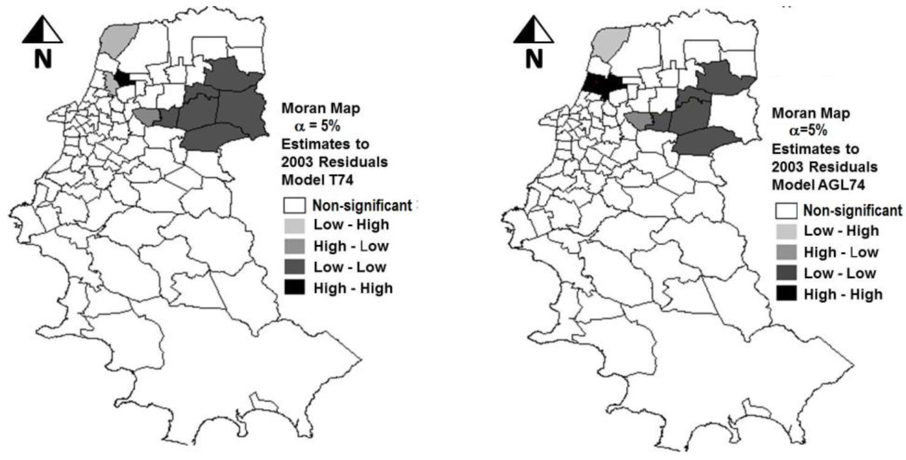
The sequence of the study was the application of the model AGL74 for future estimations. The dataset of the 2003 O-D survey was then used to check the performance of the model. Those actual values were also compared to the estimates obtained with the model T74. The HBTP values estimated with the two models for 2003 were considerably lower. They represented 59% (model AGL74) and 55% (T74 model) from those observed in reality (EDOM 2003). Those results may indicate that the coefficients of the variables in the two models adjusted for 1974 are underestimating the phenomenon under analysis. 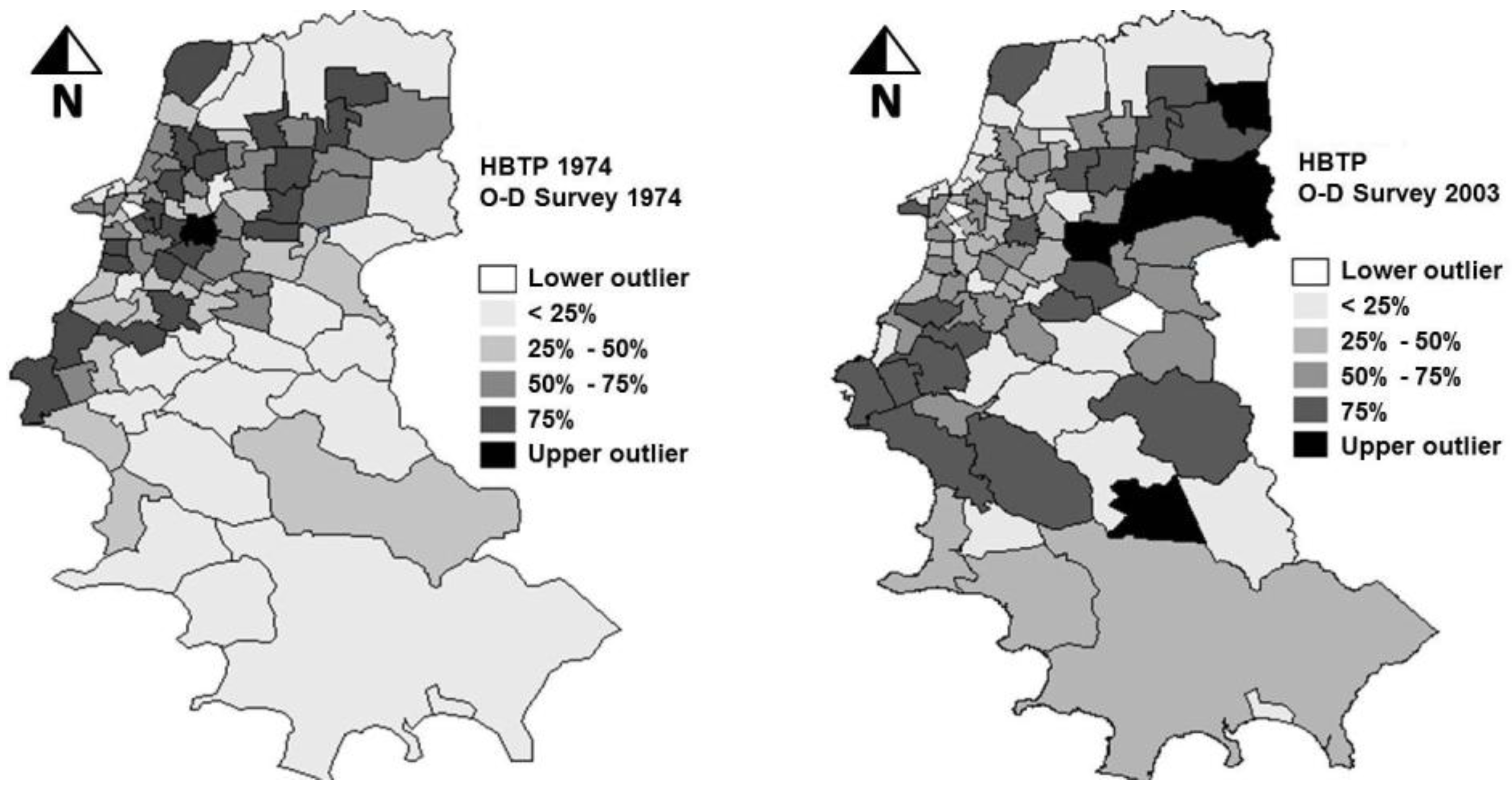The high values of errors in the estimations for 2003 can be confirmed by the analysis of Figure 2, in which clusters of zones with significant High-High residual values (high values surrounded by high values) were found. That could have been caused by the dynamics of urban development, in two ways: through changes in the relationships between different variables affecting the phenomena under study, and also through changes in the spatial patterns over that period of nearly 30 years. The thematic maps of Figure 3 show the changes in spatial patterns of home-based trip productions that actually occurred from 1974 to 2003. While in 1974 the areas with the largest number of trips were predominantly concentrated around the CBD, in 2003 they were distributed over the eastern, southwestern and southeastern parts of the city.

Figure 1. Spatial distribution of the residuals of the estimates obtained with models T74, ERR74 and AGL74 when compared with the actual data of 1974 (α = 5%; calibration phase).

Figure 1. Spatial distribution of the residuals of the estimates obtained with models T74, ERR74 and AGL74 when compared with the actual data of 1974 (α = 5%; calibration phase).

4.5. Multiple Regression-Traditional Model with the 2003 Dataset (T03)

The traditional modeling approach applied to the 1974 dataset, and described in Section 4.1, was also used to build the model T03 with the 2003 dataset (as shown in the right part of Table 2). The comparison of the coefficients of the two models, however, has shown large differences in the values. There was a considerable difference for the variable POPst (3.4 times higher for T03 than for T74) and for the constant term of the model (1.8 times higher for T03 than for T74). The variable FLEETst, which was the second traditional variable included in the model, however, had similar values for both models, in terms of magnitude. Considering that the values of the variables were standardized in both periods, these results indicate that the impact of the population (POPst) on transport demand was larger in 2003 than in 1974, while the impact of the car fleet (FLEETst) was nearly the same in both time periods.

As can be seen in Table 2, the adjusted R-squared value of model T03 was equal to 0.97. This is an indication that the variance of the dependent variable HBTP is satisfactorily captured by the model. Student’s t-tests indicated that all parameters of the T03 model were statistically significant at the 0.05 level. The multicollinearity condition number was 2.975, suggesting that the independent variables were not highly correlated. The same tests used to analyze the errors of the other models were also applied to model T03. The results of these tests confirmed that the hypotheses of normal distribution and homoscedasticity were not rejected at a level of 5% of significance. As the hypothesis of no spatial autocorrelation was rejected, the formulation of spatial models was indicated. A spatial lag model and another spatial error model, called LAG03 and ERR03, respectively, were built (as detailed in Table 2).

Figure 2. Spatial distribution of the residuals of the estimates obtained with models T74 and AGL74 when compared with the actual data of 2003 (α = 5%; validation phase).

Figure 2. Spatial distribution of the residuals of the estimates obtained with models T74 and AGL74 when compared with the actual data of 2003 (α = 5%; validation phase).

Figure 3. Spatial distribution of home-based trip productions HBTP in 1974 and 2003. Map based on the Box Plot with outliers above and below 1.5 times the interquartile range.

Figure 3. Spatial distribution of home-based trip productions HBTP in 1974 and 2003. Map based on the Box Plot with outliers above and below 1.5 times the interquartile range.

4.6. Spatial Regression-Spatial Autoregressive Model with the 2003 Dataset (LAG03)

The estimated value of the spatial autoregressive coefficient (λ) for the LAG03 model was 0.084. The z test has indicated λ, as well as the other parameters of the model, as significant. Moreover, the Breusch-Pagan test rejected the hypothesis of constant variance for the residuals and the log-likelihood (LIK) rejected the hypothesis of non-existence of spatial autocorrelation. Thus, the results suggested that this model (LAG03) was not appropriate to replicate the 2003 data.

4.7. Spatial Regression-Spatial Error Model with the 2003 Dataset (ERR03)

For the ERR03 model, the λ (W_HBPT) value of 0.457 and the other estimated parameters were indicated as significant by the z test. The hypotheses of homoscedasticity and non-existence of spatial autocorrelation were rejected by the Breusch-Pagan test and by the log-likelihood (LIK), respectively. As a result, the model ERR03 was also not accepted for the purposes of this study.

4.8. Multiple Regression-Alternative Global Local Model with the 2003 Dataset (AGL03)

The next step was the addition of local and global indicators of spatial dependence as independent variables, in the same way it was done for the 1974 dataset (as discussed in Section 4.3), what resulted in the model AGL03 (Table 2). With the exception of the estimated coefficients for LISA_DPOPst and LISA_DHHst, all other parameters were significant at a significance level of 5%. The adjusted R-squared value obtained was equal to 0.98 and the assumptions of normality and homoscedasticity of the errors were not rejected at a level of 5% of significance. The multicollinearity condition number was 9.386, suggesting that the independent variables were not highly correlated. The hypothesis of spatial autocorrelation was rejected.

A summary of the models’ characteristics and the results of the respective statistical tests are presented in Table 2. The best results are highlighted. Given that model AGL03 presented the highest LIK value and the lowest AIC and SC values, the model is better than the other three attempts with the 2003 dataset, regarding the quality of the adjustment. As in the case of the 1974 dataset, the inclusion of spatial variables and the subsequent adjustment by ordinaries least squares led to a better quality of adjustment also for the 2003 dataset.

As discussed earlier, the idea of calibrating the models with the 2003 dataset but considering the same variables of the model adjusted to the 1974 dataset was to determine the impacts of the model structure on its coefficients and performance. However, despite the good results of model AGL03, two of the three spatial variables included were not significant. That suggested the need for further investigation in order to look for additional variables that could better represent the 2003 data. Thus, a model for 2003 was also built by means of a stepwise algorithm, similarly to what has been done with the 1974 dataset and that resulted in model AGL74.

4.9. Alternative Global Model with the 2003 Dataset (AG03)

The very last model tested was a multiple regression model including global indicators of spatial dependence as exploratory variables. The search for the best model began with 18 candidate variables. Six were traditional variables, three were local indicators of spatial dependence and nine were global indicators of spatial dependence. The process resulted in a model named AG03, which is presented in Table 3. After the application of the stepwise forward regression method, a global indicator of spatial dependence (DPOP_Q2) was also found significant. Therefore, it was included in the model, in addition to the traditional variables POPst, FLEETst and HHst. The traditional variables represent, respectively, the standardized values of population, car fleet, and households per TAZ. The spatial variable DPOP_Q2 represents TAZs with population density values in quadrant 2 (i.e., the Low-Low values in a Moran scatterplot), which is an indicator of global spatial association. The model performed satisfactorily in all tests, as can be seen in Table 3. Also, the values of LIK, AIC and SC, as well as the MRE, were better than those found for the previously adjusted model AGL03.

Table 3. Summary of the best adjusted model for HBTP when considering 2003 data.

Results of the Calibration			Alternative Model
			AG03
Coefficients	“Traditional” variables	Constant	22,947.23 (<0.0001)
		POPst	7386.85 (<0.0001)
		FLEETst	1305.66 (0.0040)
		HHst	7385.37 (<0.0001)
	Global indicator of spatial dependence	DPOP_Q2	−1538.43 (0.0027)
Goodness-of-fit		R2	0.98
		Adjusted R2	0.98
		LIK	−815.86
		SC	1654.23
		AIC	1641.73
		MRE	10%
Presence of multicollinearity		Multicollinearity condition number	13.307
Absence of spatial dependence supposition (α = 5%)		LM (error)	Accepted (0.750)
		Robust LM (error)	Accepted (0.628)
		LM (SARMA)	Accepted (0.577)
		LM (Lag)	Accepted (0.352)
		Robust LM (Lag)	Accepted (0.317)
Identification of spatial dependence (α = 5%)		Moran’s I (error)	0.02 (0.455)
Normal distribution supposition (α = 5%)		Jarque-Bera	Accepted (0.866)
Homoscedasticity supposition (α = 5%)		Breusch-Pagan	Accepted (0.126)
		Koenker-Bassett	Accepted (0.171)

Note: ( ) p-value of the respective significance test.

Table 3. Summary of the best adjusted model for HBTP when considering 2003 data.

Results of the Calibration			Alternative Model
			AG03
Coefficients	“Traditional” variables	Constant	22,947.23 (<0.0001)
		POPst	7386.85 (<0.0001)
		FLEETst	1305.66 (0.0040)
		HHst	7385.37 (<0.0001)
	Global indicator of spatial dependence	DPOP_Q2	−1538.43 (0.0027)
Goodness-of-fit		R2	0.98
		Adjusted R2	0.98
		LIK	−815.86
		SC	1654.23
		AIC	1641.73
		MRE	10%
Presence of multicollinearity		Multicollinearity condition number	13.307
Absence of spatial dependence supposition (α = 5%)		LM (error)	Accepted (0.750)
		Robust LM (error)	Accepted (0.628)
		LM (SARMA)	Accepted (0.577)
		LM (Lag)	Accepted (0.352)
		Robust LM (Lag)	Accepted (0.317)
Identification of spatial dependence (α = 5%)		Moran’s I (error)	0.02 (0.455)
Normal distribution supposition (α = 5%)		Jarque-Bera	Accepted (0.866)
Homoscedasticity supposition (α = 5%)		Breusch-Pagan	Accepted (0.126)
		Koenker-Bassett	Accepted (0.171)

Note: ( ) p-value of the respective significance test.

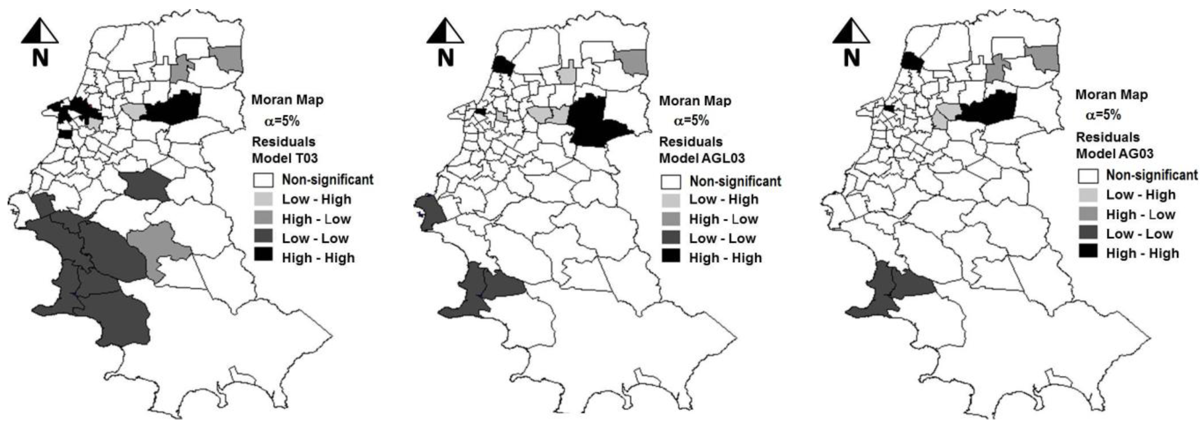
Figure 4. Spatial distribution of the residuals of the estimates obtained with models T03, AGL03 and AG03 when compared with the actual data of 2003 (α = 5%).

Figure 4. Spatial distribution of the residuals of the estimates obtained with models T03, AGL03 and AG03 when compared with the actual data of 2003 (α = 5%).

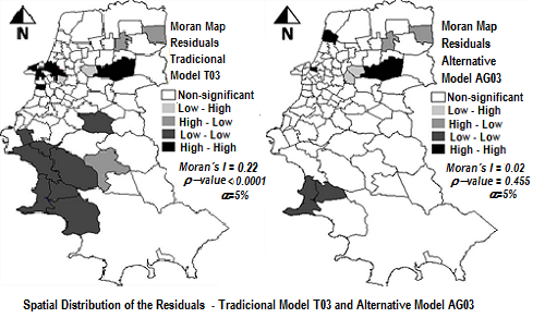
Therefore, this study confirmed the assumption that the inclusion of indicators of spatial dependence among the variables could improve the predictive power of the model. The Moran Maps in Figure 4, which highlight the areas with significant groupings of high or low values of estimation residuals, also show the superiority of the alternative models AGL03 and AG03 in comparison to the traditional model T03. The T03 model shows several areas grouped in regions with high absolute values of residuals, indicating a tendency to underestimate or overestimate the number of trips in certain regions.

5. Conclusions

The results of the application in the city of Porto Alegre indicated that the alternative models (i.e., spatial regression models or regression models including spatial variables) performed better than the traditional models. Therefore, the effects of spatial dependence in regression models are important and must be explicitly considered. That was observed in the models built using both 1974 and 2003 datasets.

AGL models are multiple regression models that contain spatial variables (both global and local) as independent variables. AGL74 was the model that best fitted the data of 1974. Similarly, AGL03 was initially the model that showed the best results for the 2003 dataset. Subsequently, however, the examination of the most significant variables for 2003 led to the development of model AG03, which become the best adjusted option for the 2003 dataset. Hence, the inclusion of spatial variables, such as global and local indicators of spatial dependence, in the specification of the model and a subsequent adjustment by Ordinaries Least Squares was the best alternative in the case analyzed. Also, according to Getis and Griffith [37], this approach makes results more directly comparable with those of more traditional statistical methods.

However, long-term forecasts in fast growing cities, such as in the case discussed here, may not be well represented by the models. The significant changes observed in the urban settings of Porto Alegre are certainly among the reasons why the results obtained with model AGL74 were only slightly better (and not significantly better) than the results obtained with the other models. We believe that the consideration of the effects caused by the dynamics of urban development in transportation demand modeling can further improve the results.

A comparison of the coefficients of the models adjusted for 2003 with those adjusted for 1974 has shown significant changes in the variables’ relationships in that period of nearly three decades. The weight of population, for example, which is an explanatory variable to home-based trip productions, was much higher in 2003 than in 1974. There were also changes in the spatial patterns of the trips in the different periods. Their analyses may help to better understand the dynamics of urban development, for later improving the models discussed here.