Article

Model for Determining Geographical Distribution of Heat Saving Potentials in Danish Building Stock

Department of Management Engineering, Technical University of Denmark, Frederiksborgvej 399, Building 130, Roskilde 4000, Denmark
*
Author to whom correspondence should be addressed.
ISPRS Int. J. Geo-Inf. 2014, 3(1), 143-165; https://doi.org/10.3390/ijgi3010143
Submission received: 30 November 2013 / Revised: 15 January 2014 / Accepted: 20 January 2014 / Published: 5 February 2014
(This article belongs to the Special Issue GIS for Renewable Energy)

Abstract

:
Since the global oil crisis in the 1970s, Denmark has followed a path towards energy independency by continuously improving its energy efficiency and energy conservation. Energy efficiency was mainly tackled by introducing a high number of combined heat and power plants in the system, while energy conservation was predominantly approached by implementing heat saving measures. Today, with the goal of 100% renewable energy within the power and heat sector by the year 2035, reductions in energy demand for space heating and the preparation of domestic hot water remain at the top of the agenda in Denmark. A highly detailed model for determining heat demand, possible heat savings and associated costs in the Danish building stock is presented. Both scheduled and energy-saving renovations until year 2030 have been analyzed. The highly detailed GIS-based heat atlas for Denmark is used as a container for storing data about physical properties for 2.5 million buildings in Denmark. Consequently, the results of the analysis can be represented on a single building level. Under the assumption that buildings with the most profitable heat savings are renovated first, the consequences of heat savings for the economy and energy system have been quantified and geographically referenced. The possibilities for further improvements of the model and the application to other geographical regions have been discussed.

1. Introduction

The Danish energy system could be seen as flexible, highly efficient, with a large amount of renewables, and almost self-sufficient. However, in order to gain a full overview of the Danish energy system, it should be seen from a historical point of view and should be put in the context of a never-stopping transition towards a 100% renewable energy system.
Before the first global oil crisis in 1973, Denmark was almost entirely dependent on imported oil. At that time, oil was responsible for 92% of total primary energy consumption. A large part of the transportation and residential heating sector was based on oil, while at that time, the oil share in electricity production was close to 78%; the rest of the electricity was produced from coal [1]. Denmark did not have a ministry of energy to create medium- and long-term planning strategies, so “energy planning” was based on the analysis of historical demand for energy, without attempting to “put the bound” on the raising demand. The proclamation of an oil embargo by the Arab petroleum-exporting countries harmed the Danish economy at that time, but it also denoted the beginning of energy planning.
heat savings in the building (if not specified otherwise, the term building is used in a general way and denotes any kind of construction that has an energy demand for heating and hot water preparation, disregarding the size, number of floors or use) stock have been introduced as a part of the Danish energy strategy in the first major policy statement published by the Ministry of Trade in 1976. That strategy had declared two main directions for fighting the dependency on imported oil energy efficiency and energy conservation. The plans for energy efficiency improvements included converting existing power plants to CHPs (combined heat and power) and installing district heating technologies. Plans for energy conservation were mainly based on heat savings within the building sector. The burning issue of dependency on imported fuel was approached by introducing coal, natural gas, nuclear power and renewable energy as a primary energy substitute for imported oil. Soon after, nuclear power was taken off the agenda in Denmark, and societal consensus about this topic is maintained until the present time.
From a current point of view, the Danish energy system has been successfully converted from an inefficient, oil-based one to an efficient energy system based on renewable energy. Transition is still ongoing as Denmark is heading towards a 100% renewable energy system by 2050, which is a widely accepted societal consensus in Denmark. If the building sector is analyzed as a separate system, then Lund [2] points out an extraordinary result: even though the heated area in buildings increased by more than 50% during the last four decades, the total heat demand has decreased by 27%. In 2011, the final energy consumption for space heating was around 202 PJ, corresponding to one fourth of the total energy consumption in Denmark. Therefore, there is still room for reductions in energy demand for space heating and domestic hot water preparation. In theory, almost the entire energy consumption for space heating could be avoided. Naturally, the extremely high costs of insulating such buildings limit the applicability of these solutions in theory. The results of comprehensive analysis presented in [3] show that it is economically feasible to reduce energy demand for space heating by 30% in the next 15 years and by 80% until 2050. Net zero energy buildings described in [4] with a space heating demand of around 15 Ijgi 03 00143 i017 and 18 Ijgi 03 00143 i017 of hot water demand provide an indication of how far it is possible to go with new buildings. Due to the high share of district heating in Denmark, which covers around 60% of Danish heating needs, an important aspect of any system-changing measure is its ability to work alongside district heating. Several studies [5,6,7] have concluded that heat savings in the building stock will work well with district heating, today, as well as in a future renewable energy system, when the share of district heating increases even more. A lower heat demand in buildings will enable the introduction of fourth generation district heating technologies with lower supply and return temperatures, thus reducing the major disadvantage of district heating transmission losses.
Denmark’s striving towards a 100% renewable energy system could be seen as a part of a general, European tendency to develop towards a more energy-secure and efficient, low-emission, renewable energy future. In 2009, as a supporter of the common future, Denmark was among the EU member states to adopt mid-term targets in areas of renewable energy, energy efficiency and emission reductions (commonly known as EU 20-20-20 goals):
  • Decrease the emission of greenhouse gasses by 20% in comparison to 1990 levels by 2020.
  • By 2020, 20% of the EU’s final energy demand should be covered by renewable energy, such as wind, solar, wave and biomass. Denmark went even further with its renewable energy targets, setting the 2020 goal for the share of renewable energy of final energy demand to 30%.
  • Decrease total energy consumption by 20% by improving energy efficiency in the whole chain of production-transmission-distribution-end-use compared to the business-as-usual scenario [8].
The objectives of the present article are:
  • To identify potentials and associated costs of heat savings within the Danish building stock and to assess its effects on the energy system and environment.
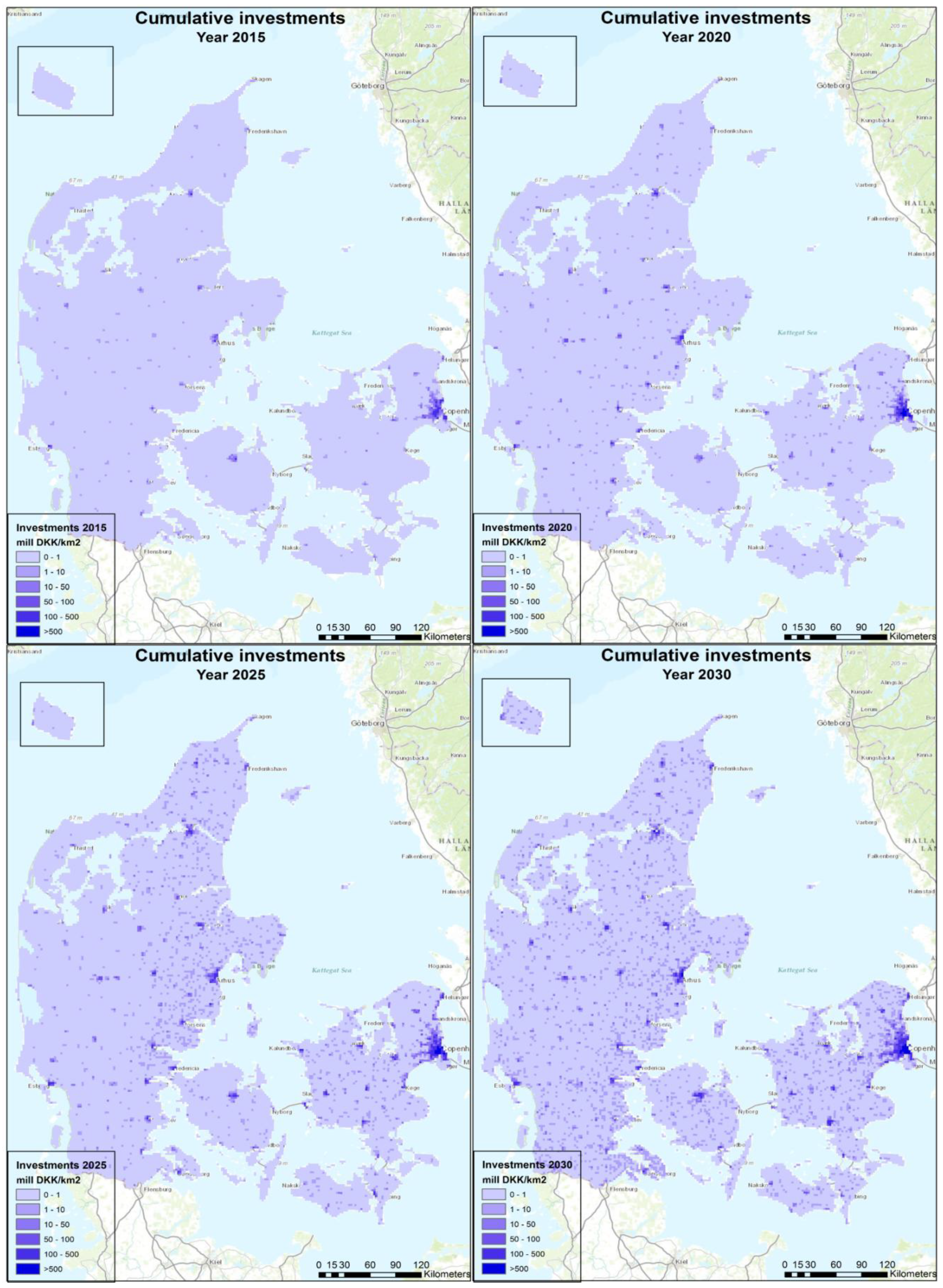
  • To put the effects of heat savings on the economy and the energy system into a spatial context.

2. Methodology and Tools

To reach the first objective of the present article, a model based on the physical properties of buildings is created. Buildings are put into groups in order to represent the different variations of physical characteristics within the building stock. The heat demand was calculated on a monthly level by using simple physical equations and summed to get the yearly demand. Different steps of heat saving measures (in the present paper, called “levels”) have been selected, and associated energy savings and costs have been identified. These results have been translated into marginal cost curves. In order to be able to compare these with the costs of current ways of supplying heat, the costs of heat saving measures have been discounted over their respective lifetimes using a socio-economic discount rate.
To reach the second objective of the paper, the Danish heat atlas [9] was used as a backbone. Since the model’s results have been calculated within a Microsoft Access database on a single building level, the spatial coordinates of buildings have been used to spatially represent the obtained results in ArcMap 10.1 software. An economically rational scenario about the renovations of buildings has been assumed, and its consequences have been used to present both spatial and temporal changes in a geographical context.
The heat atlas for Denmark will shortly be described in the following section, while a detailed description of the heat savings model will follow in subsequent sections.

The Danish Heat Atlas

The heat atlas for Denmark has been developed at Aalborg University and used in multiple studies (unless otherwise specified, the Danish heat atlas refers to this version of the heat atlas throughout this paper) [5,6,7,10]. It contains spatially referenced information about Danish building stock, including data about age, area, use, installation and fuel used for heating, preservation status, etc. It also contains calculated heat demand and the costs of different levels of heat savings. The research presented in the current paper uses the Danish heat atlas as a source of data about building stock; however, the calculated energy demand for heating and domestic hot water preparation and the costs of heat savings contained in the heat atlas are not used. Instead, a detailed model is created and thoroughly elaborated in the following sections.

3. The Heat Savings Model

To analyze heat demand for space heating and domestic hot water preparation within the Danish building stock, a stationary model based on monthly calculations of heat losses and heat gains is developed. Buildings are grouped according to age and use in order to account for variations in the physical properties of the building stock. The model requires a large amount of input data on physical variables, such as the areas of building elements (walls, roof, floor, windows), along with thermal characteristics (u-values), internal temperatures, ventilation rates, external temperatures, etc.
Different heat saving measures have been assumed, and for each of them, a new heat demand is calculated. Heat savings are defined as a difference between heat demands before and after undertaken measures. Empirical values obtained from a literature review have been used to calculate the costs of these measures.
The results from the model are presented in two ways, spatially and graphically. This is done in order to underline the duality between the results presented on a map and the results presented in graphs; each point on the map could be uniquely transferred to the graph, and vice versa, each point on the graph has its spatial origin.

3.1. Grouping of Buildings

For the purpose of modelling the heat demand of the Danish building stock, buildings have been grouped into nine groups by common construction period, five groups by common use and eight groups by a common temperature region, which gives a total of 360 groups of buildings, as presented in Table 1 and Table 2 and Figure 1. The Building codes shown in Table 2 represent the way the Danish Buildings and Dwellings Register (BBR) classifies buildings according to common use. The main reason for dividing buildings in this way is the availability of data, as this is the way buildings are grouped in reports made by the Danish Buildings Research Institute (SBi), which are often used as the main source of data about the physical properties of buildings. These values have been collected during the sale and rental of existing buildings and extrapolated using BBR’s and Danish Statistics’ data to match the five groups presented in Table 2. By grouping the buildings into these five groups, this analysis includes around 68% of all buildings, 64% of all building area, but 84% of the heat demand in Denmark, according to values from the Danish heat atlas. Heat demand contained in the Danish heat atlas has been previously calculated according to [11,12] and verified by comparing it with Danish Energy statistics.
Table 1. Grouping of the Danish building stock by common construction period.
Construction YearBefore 18501850–19301931–19501951–19621962–19731973–19781979–19981998–2006After 2007
Year group123456789
Table 2. Grouping of the Danish building stock by common use.
Building CodeUse of buildingsUse group
110FarmhousesFarmhouses
120Detached housesDetached houses
130Terrace housesNon-detached houses
140, 150, 160, 190Blocks of flats, hostels, residential institutions, other dwellingsMultistory buildings
320, 330, 390, 420,
430, 440, 490, 530
Trade and commerce, hotel and service, other trade, cultural buildings, schools, hospitals, kindergartens, other public buildings, sports buildingsOffice/public buildings
Figure 1. Temperature regions in Denmark [13].
Ijgi 03 00143 g001

3.2. Heat Demand in Buildings

The heat demand in a single building is based on [14] and is calculated as:
Qheat(c, u, t) = Qtr(c, u, t) + Qvent(c, u, t) − Qadd(c, u) + QDHW(c, u)
where the symbols used have the following meanings.
Qheat(c, u, t): Net heat demand in a building that belongs to construction period c, usage group u and temperature region group t.
Qtr(c, u, t): Transmission losses through the building envelope.
Qvent(c, u, t): Ventilation losses.
QDHW(c, u): Heat demand for the preparation of domestic hot water.
Qadd(c, u): Heat gain received from solar radiation, human body heat and surplus heat from electrical appliances.
Transmission losses through the building envelope are calculated as:
Ijgi 03 00143 i001
where the used symbols have the following meaning.
uelem(c, u, t): u-value Ijgi 03 00143 i012 of a specific element of the building envelope (wall, floor, roof, window).
A: Heated area of a specific building.
tind(c, u): Indoor temperature; the values are based on [15].
k24 = 0.024: The coefficient that incorporates multiplying by 24 h in a day and dividing by 1,000, so that Qtr is expressed in kWh.
Ijgi 03 00143 i020: The reduction factor due to the possibility that the temperature on the external side of a building envelope’s element is different from the outdoor temperature. A value of 0.7 is taken for floors and one for walls, roofs and windows. The numerical values are based on [16].
felem(c, u): The ratio between the area of a specific building element and the heated area of the building. It has been calculated based on example buildings from [17].
tout,m(t): Average outdoor temperature in months, m, and temperature region t. Values are based on [13] for eight temperature regions in Denmark.
dm: The number of days with heating in months, m. It is assumed that heating is provided from September to May, as stated in Table 3.
Table 3. The number of days with heating per month.
Month in Heating SeasonNumber of Days with Heating
January31
February28
March31
April30
May18
September6
October31
November30
December31
Ventilation losses from buildings are calculated as:
Ijgi 03 00143 i002
where the symbols used have the following meaning.
ƞ(c, u): The efficiency of heat recovery; natural ventilation or ventilation without heat recovery is assumed as stated in [17]. Same values for the efficiency of heat recovery have been assumed for multi-story and office/public buildings.
Ijgi 03 00143 i013: The density of indoor air.
Ijgi 03 00143 i014: The thermal capacity of indoor air.
Ijgi 03 00143 i015: The air flow rate.
n(c, u): The air exchange rate. The numerical values are based on [15].
H (u): The average room height. The numerical values are based on [15].
Other symbols used in Equation (3) have been explained above.
Heat gained from solar radiation, human body heat and waste heat from electrical appliances is calculated as follows:
Ijgi 03 00143 i003
where the used symbols have the following meaning
Qint, Qsol: The internal heat gain (from human body heat and electrical appliances) and the solar heat gain, respectively.
Ijgi 03 00143 i016: The heat gain from human body and waste heat from electrical appliances. The same value is assumed for residential and office/public buildings. The values are taken from [14].
ƞh: The utilization factor of heat gains; based on a graph from [18].
psol: The solar radiation per area of windows. For calculations presented in the current paper, the average values for all orientations of windows are calculated from [14].
Fs: The reduction factor due to shadowing effects, based on [18].
Fa: The reduction factor due to the entire glass area being less than the total window area, based on [18].
Fg: The reduction factor due to the solar transmittance of windows, based on [18].
All other factors are used earlier and have already been explained.
Heat demand for domestic hot water is calculated as follows:
  • for office/public buildings:
    Ijgi 03 00143 i004
  • for residential buildings:
    Ijgi 03 00143 i005
where Q Ijgi 03 00143 i024 and Q Ijgi 03 00143 i023 denote the energy demand for hot water in office/public and residential buildings, respectively q Ijgi 03 00143 i024. is heat consumption for hot water per unit of heated area in office/public buildings, while q Ijgi 03 00143 i023 represents heat consumption for domestic hot water per apartment in residential buildings. r(c,u) represents the average area of households in usage group u, constructed in time period c. It is calculated as a ratio between the total number of households of a specific type and the total heated area of buildings of the same type. The total number of households of a specific usage group and construction period is obtained from Danish Statistics, while the total heated area of buildings of a specific type is taken from [19]. As before, A represents the heated area of a building.
The reason for using different ways of calculating Q Ijgi 03 00143 i024 and Q Ijgi 03 00143 i023 in Equations (5a) and (5b) is that q Ijgi 03 00143 i024(c) is calculated in Ijgi 03 00143 i017 per year, while q Ijgi 03 00143 i023(c, u) is calculated in Ijgi 03 00143 i021 per year, and the intention was to present both in Ijgi 03 00143 i017 per year. Both q Ijgi 03 00143 i023(c, u) and q Ijgi 03 00143 i024(c) are based on actual measurements published in [20,21].
The calculated energy demand for space heating and domestic hot water has been compared with data in Danish Energy Statistics and data previously contained in the Danish heat atlas prior to calculation. It has been observed that the mismatch between total heat demands amounts to 0.2%, while mismatches divided in five building groups presented in Table 2 amount to 25.2% in the case of non-detached houses. Comparison is done only for buildings included in the calculation. The results of the comparison are presented in Table 4. When compared to Danish Energy Statistics, this analysis shows that the analyzed buildings make up 78% of the heat demand in Denmark.
Table 4. Comparison between the calculated heat demand and the heat demand previously contained in Danish heat atlas.
Use GroupQheat (TWh)Qheat atlas (TWh)Ratio (%)
Detached houses16.6417.6294.4
Farmhouses2.62.49104.4
Multi-story buildings12.5410.79116.2
Non-detached houses2.323.0675.8
Office/public buildings9.699.9197.8
SUM43.7943.8799.8

3.3. Heat Savings

After determining energy demand for space heating and domestic hot water, the next step is to determine the possibility for reducing energy consumption. In theory, it is possible to reduce the heat demand almost to zero, but clearly, this cannot be economically justified. Therefore, a list of heat saving measures is made, and the heat savings and associated costs are calculated for each of these measures. The complete list of heat saving measures is presented in Table 5.
Heat savings are separately calculated for all elements and all levels listed in Table 5 using the following equations:
Equation (1) for exterior walls, floors and roofs is:
Ijgi 03 00143 i006
Table 5. Description of different heat saving measures
ElementLevelAdditional Insulation Thickness 1 (mm)
wallLevel 1100
wallLevel 2150
wallLevel 3200
roofLevel 150
roofLevel 2100
roofLevel 3150
windowLevel 11.5
windowLevel 20.8
windowLevel 3 21.3
floorLevel 1100
ventilation systemsLevel 10.9
domestic hot waterLevel 140
domestic hot waterLevel 250
1 In case of windows, u-value of installed windows is written, while in case of mechanical ventilation systems efficiency of heat recovery of newly installed system is noted.2 In contrast with other heat saving measures where higher levels are denoting better insulated elements of building envelope, “level 3” in windows represents internal windows, which are used in case existing windows are worth preserving.
Heat savings in these elements are achieved by adding additional insulation, resulting in a lower u-value of the specific element. The nonlinear relationship between insulation thickness in walls, floors and roofs and their u-values is taken from [22,23]. It is assumed that in buildings that previously had an indoor temperature of tind,old = 19 °C, the indoor temperature had increased to tind,new = 20 °C and, thus, reduced the effects of heat savings but increased living comfort. For buildings with higher values for tind,old than 19 °C, no change in indoor temperature is assumed.
Equation (2) for windows is:
Ijgi 03 00143 i007
Heat savings in windows are achieved by installing windows with a lower u-value. As before, an increase in indoor temperature from 19 °C to 20 °C is assumed, while it is assumed that there is no change in indoor temperature in buildings with an indoor temperature greater than or equal to 20 °C before renovation. The effect of installing new windows on solar gains is acknowledged through the change in factors Fa and Fg. The change of factor Fa denotes the change in the glass area relative to the window area, while factor Fg (closely related with the g-value of the window) denotes the change in the solar transmittance of windows when switching to more energy efficient windows.
Equation (3) for ventilation systems is:
Ijgi 03 00143 i008
Reductions of ventilation losses are achieved by installing mechanical ventilation systems with heat recovery. An efficiency of heat recovery of 0.9 is assumed for all newly installed ventilation systems. An increase in indoor temperature from 19 °C to 20 °C is also assumed in the case of mechanical ventilation systems. Apart from the decrease in energy consumption for air heating, the installation of mechanical ventilation system can contribute to improved air quality.
Equation (4) for domestic hot water pipes is:
Ijgi 03 00143 i009
Ijgi 03 00143 i010
where po(%) and pr(%) denote the percentages of pipes being insulated in office/public and residential buildings, respectively. In heat saving calculations presented in this paper, a percentage of 20% is assumed for all types of buildings. This percentage is applied as a conservative one and should account for inaccessible hot water pipes in buildings. lo(c, u) and lr(c, u) are the average lengths of pipes per the heated area of building that belong to usage group u and are built in construction period c. These values represent calculated averages based on [20,21]. Ijgi 03 00143 i018 represents energy savings per length of pipe being insulated, depending on the insulation thickness. Assumptions from [17] have been applied.
As thoroughly explained in [20], energy consumption for domestic hot water represents a high percentage of the total energy consumption in residential buildings in Denmark: around 50 TJ out of a total of 200 TJ. Around 10% of gross energy consumption for domestic hot water is losses in hot water tanks, 40% are circulation losses, while net consumption represents only 50%. Although this calculation shows that the insulation of hot water pipes is an inexpensive solution, the total amount of energy that can be saved by this measure appears to be relatively low, as it changes from building to building, but does not exceed 5% of the total energy demand for hot water. Stopping the circulation of water during the night or reducing the length of circulating pipes would have a larger impact on the reduction of such losses, but these effects are impossible to include from a system point of view. On the other hand, solar heating appears to be a promising solution for supplementary heating of hot water, and analysis of this option for reducing energy consumption remains an open topic for further research. Additionally, the functionality of the Solar Radiation Toolset in ArcGIS 10.1 could be fully utilized for the benefit of this analysis.

3.4. Costs of Heat Savings

A logical question that follows from the results of the heat saving calculations is “How much does it cost?” As previously mentioned, it is theoretically possible to reduce heat demand for space heating almost to zero, but only if economic aspects are not taken into account. In order to make an economic assessment of heat saving measures, marginal and full costs are calculated. Marginal costs are supposed to account for additional costs when a scheduled renovation takes place, while full costs account for costs when renovations takes place only for the sake of saving energy. Because of the legal obligation to achieve high standards of energy efficiency when renovating buildings in Denmark, marginal costs are lower than full costs. As a drastic example, marginal costs of replacing windows to level 1 are considered to be zero, as would be done anyway when a scheduled renovation takes place. The numerical values assigned to marginal and full cost for walls, floors and roofs are based on [24,25], for windows on [16,24], for mechanical ventilation systems with heat recovery on [25] and for insulating hot water pipes on [16]. These values are grouped and presented in Table 6.
Table 6. Marginal and full costs of different heat saving measures.
ElementMarginal Costs Ijgi 03 00143 i0191Full Costs Ijgi 03 00143 i019
wall7 × ∆d 21,500 + 7 × ∆d
roof50 + ∆d100 + ∆d
floor350350
window, level 102,500
window, level 21,5004,000
window, level 32,0003,000
ventilation system with heat recovery300300
hot water pipes 3, level 1 100100
hot water pipes, level 2120120
1 exchange rate: 1 EUR = 7.45 DKK; 2d is additional insulation thickness; 3 In case of hot water pipes costs are expressed in DKK per m of pipe being insulated
In order to assess the economically feasible potential seen from a system point of view, the costs of heat saving measures have been discounted over the lifetime of each measure. Forty years is assumed as the lifetime of walls, floors and roofs, while 30 years has been assumed as the lifetime of windows, ventilation systems and the insulation of hot water pipes. A 4% socio-economic discount rate has been assumed, as stated in [26]. Lower interest rates [27,28,29] and longer lifetimes [3] of elements can be found in the literature, which makes the economically feasible potential higher.
Annualized discounted marginal and full costs have been calculated for all buildings included in this analysis and for all twelve heat saving options presented in Table 5, by applying the following equation:
Ijgi 03 00143 i011
where the used symbols have the following meaning.
IC: The investment costs calculated by using values from Table 6.
AC: The discounted annualized cost of a heat saving measure.
CRF: The capital recovery factor.
I: The interest rate.
N: The lifetime of the building envelope element.

4. Results of Analysis

After applying Equation (10) on the marginal and full costs of each level of each heat saving measure of each building included in the analysis, the marginal and full annualized costs of heat saving measures are obtained.
Figure 2. Cumulative potentials and marginal costs of different heat saving measures.
Ijgi 03 00143 g002
From knowing the discounted price of heat saving measures (in Ijgi 03 00143 i022
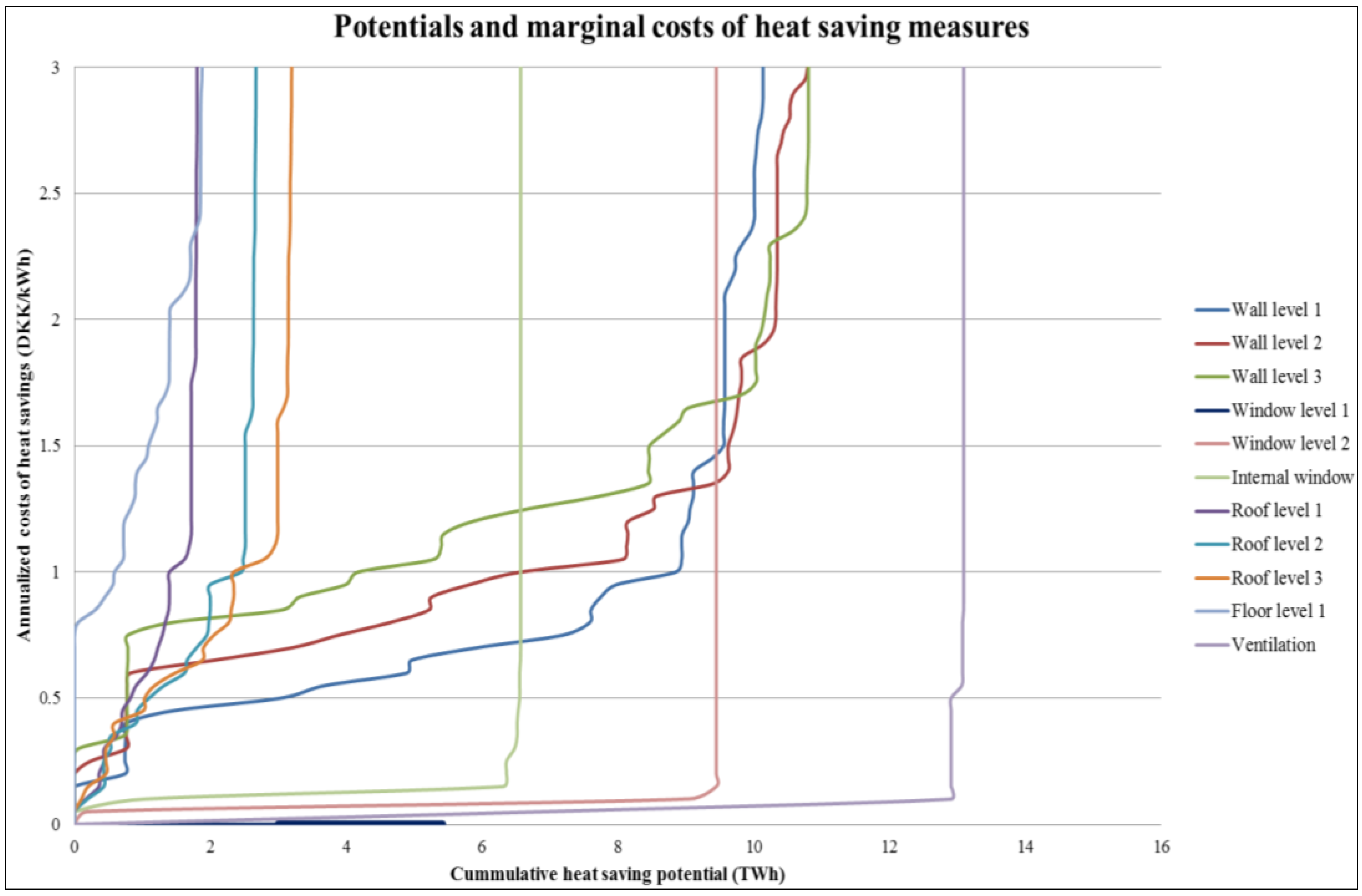
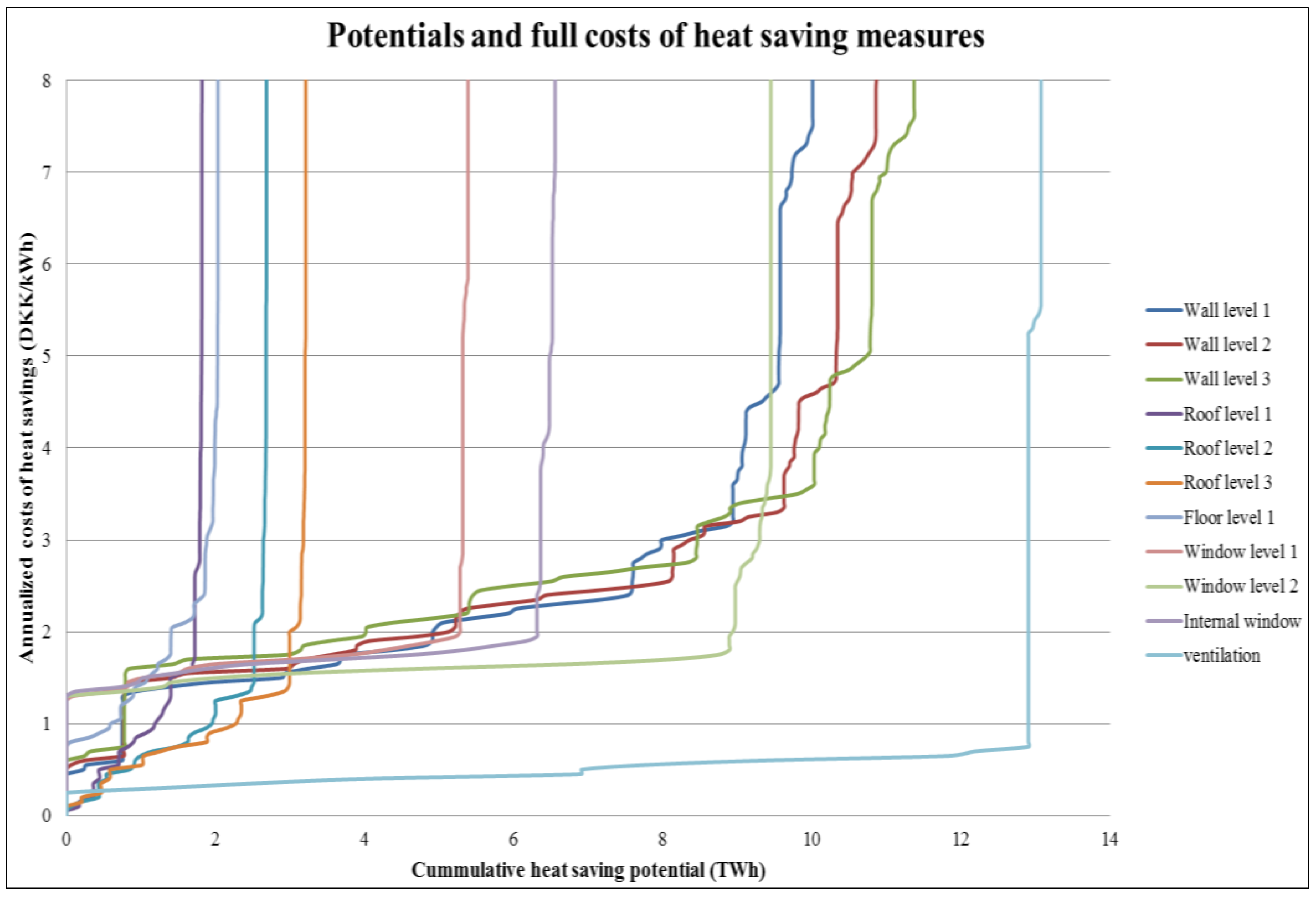
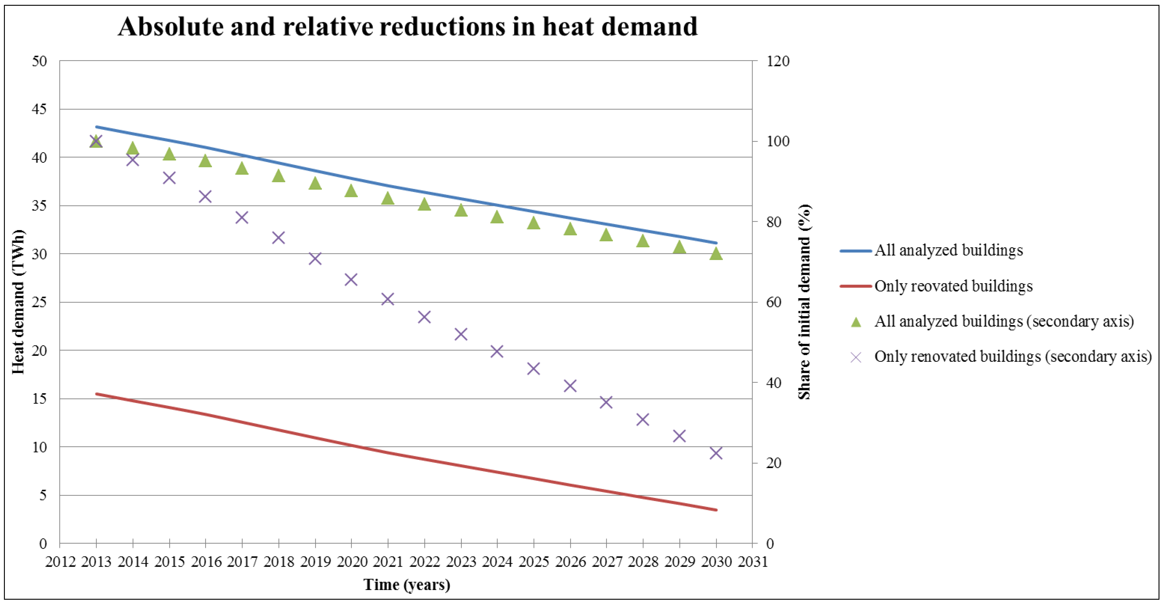
) for all buildings, the next step in the analysis is to answer the question “How big is the potential for heat savings?”. In order to provide an answer to this question, marginal cost curves have been created (It is important to make a clear distinction between marginal cost curves and marginal costs. Marginal cost curves show the costs of savings next to the unit of energy, while marginal costs denote the costs of heat saving measures when a scheduled renovation is taking place). For each heat saving level of each element on all buildings included in the analysis, costs have been sorted from the least to the most expensive one. These curves are presented in Figure 2 and Figure 3. Curves showing potentials and costs for energy savings in domestic hot water are not presented in Figure 2 and Figure 3, due to the small potential (0.1 TWh), even though they show moderate costs (around 1 DKK per saved kWh). After picking only the most profitable (the smallest amount of money that is needed to save 1 kWh of heat) heat saving measure for each element on all buildings, the curves in Figure 4 are obtained. This analysis allows for the possibility that on the same element in the same building, one level of savings appears more profitable when a scheduled renovation is undertaken, while some other level appears more profitable when renovation is undertaken solely for the purpose of saving energy. For example, it is possible that adding 100 mm of insulation on walls (level 1) appears as the optimal solution if marginal costs are calculated and 300 mm if full costs are considered. As a result of that, the total potential when renovation for energy saving purposes is considered is 12% higher than in the case of a scheduled renovation, as presented in Figure 4.
Figure 3. Cumulative potentials and full costs of different heat saving measures.
Ijgi 03 00143 g003
Figure 4. Cumulative potentials and marginal and full costs of heat savings without disaggregation on different building elements.
Ijgi 03 00143 g004

5. Analysis of Results

The calculations presented in previous chapters explained and quantified heat saving potentials within the Danish building stock and the associated costs. However, still, many issues are left open; some of these include the temporal and spatial distribution of heat saving measures and associated investment costs and the environmental and energy system consequences.
It seems that some of the mentioned questions have rather simple answers, which could be interpreted as follows: heat savings save energy, which is produced in a power plant and transmitted and distributed to buildings, with some losses, and consumed in the building. Another option is that heat is both produced and consumed locally, i.e., without transmission losses.
Furthermore, heat savings reduce the harmful environmental impact of heat producing technologies, such as CO2, CH4 and NOx emissions (even though CO2 is the most commonly known, others have a bigger global warming potential), except for technologies that use fuels that do not produce emissions (e.g., heat produced from electricity produced from wind power). Finally, it is evident that heat savings are not costless: new windows, ventilation systems, as well as materials for insulating walls, floors and roofs cost money, as previously presented in Table 6. However, in order to fully understand the effects of heat savings in the building stock on the Danish energy system, the previously mentioned effects should be quantified while spatial and temporal aspects should be explored. The following analysis is aimed at achieving these goals.
Economic rationality could be seen as a key underlying assumption of the decision-making process in this analysis. It is assumed that buildings with more cost-effective heat saving measures (measures that need the least DKK for saving 1 kWh of heat, placed on the bottom of the curves presented in Figure 2, Figure 3 and Figure 4) are renovated before the ones with more costly heat savings. Another factor that could greatly influence the profitability of heat saving measures is the cost of the current mean of supply, as heat savings could be deemed reasonable only if the costs of heat savings per saved kWh of heat are less than the current price of supplying heat. As an extreme case, if a building has a free heat supply, no heat saving measure would be seen as profitable. However, this effect has not been included in this analysis and should be addressed when comprehensive energy system analysis is undertaken. Gram-Hansen [30] gives another perspective to the issue of building renovations by exploring the reasons behind owner’s decisions against renovations, even in cases when it is economically feasible. The issue of the renovation rate has been addressed similarly as in [22]; it is assumed that an area corresponding to 1% of the total area of buildings is renovated as a scheduled renovation (marginal costs have been applied) and another 0.5% is being renovated for energy saving purposes (full costs have been applied). The effect of constructing new buildings has not been explored, but their effect on heat consumption is minor compared to old buildings, since these buildings are built according to the highest standards of energy efficiency. These assumptions clarify the temporal aspects of energy renovations. The present analysis looks at the results of renovation starting from the year 2013 up to 2030. Informations about the position of buildings contained in the heat atlas allow for the monitoring of spatial aspects of energy renovations; financial investments and energy savings can also be spatially referenced.
The results of the analysis have been presented in the form of density maps changing over time. The density of cumulative heat savings in milestone years has been presented in Figure 5, and the density of cumulative financial expenses in the years 2015, 2020, 2025 and 2030 have been presented in Figure 6. The Kernel density tool in ArcGIS 10.1 has been used for producing these maps. One kilometer is used as a raster cell size and as a search radius within the Kernel Density tool. A land map of Denmark has been converted to raster cells (a value of one for land and zero for the surrounding sea) and used within the Raster calculator to “remove” densities from the sea, where buildings do not exist. This kind of visual appearance is achieved by using Classified Symbology and six colors scale within Layer Properties.
Figure 5. Temporal change in cumulative heat savings within the Danish building stock.
Ijgi 03 00143 g005
Figure 6. Temporal change in cumulative financial expenses for renovations within the Danish building stock.
Ijgi 03 00143 g006
Although it could be expected that change in densities from one milestone year to another follow identical spatial patterns, it is evident from the maps shown in Figure 5 and Figure 6 that this is not entirely the case. An explanation of this phenomenon will arise from the following discussion.
Let us assume that the changes of cumulative energy saved over time, presented in Figure 5, represent the basic maps and that the other group of maps will be compared with it. Maps showing the time change in the cumulative financial expenditures for building renovations presented in Figure 6 differ from maps presented in Figure 5. There is a sound reason for that. Buildings are supposed to be renovated on the basis of the lowest costs per saved unit of energy, irrespective of the area of the buildings and the total amount of energy saved, so it is possible that inexpensive-to-renovate buildings with high a heat demand are located in one region, while expensive-to-renovate buildings with a smaller heat demand are located in another region. That is why, even though large heat savings are achieved in one region, financial expenditures are not as large and vice versa.
To underline the duality between the spatial and the graphical way of representing the results, graphs are presented in Figure 7, Figure 8 and Figure 9. The graph in Figure 7 shows the absolute (on the primary axis) and relative (on the secondary axis) change in heat demand after renovations of buildings are undertaken. It could be seen that if 1.5% of the building area is renovated annually (1% as scheduled renovation and 0.5% as energy saving renovation), the total heat demand in the analyzed buildings will decrease by 28%, while the heat demand in the renovated buildings will decrease by 78%.
Figure 7. Absolute and relative change in heat demand over the observed period.
Ijgi 03 00143 g007
Figure 8 and Figure 9 show how saved thermal energy and investments are spread over different types of buildings and different administrative regions in Denmark. When compared with the temperature regions presented in Figure 1, the Capital region is composed of Copenhagen and Bornholm, South Denmark of Fyn and South Jutland, Central and East Jutland of Central Jutland, while the temperature regions of Zealand and North Jutland correspond to homonymous administrative regions. Red points in Figure 8 denote heat savings in a certain region as a share of initial consumption in all analyzed buildings, while dark squares denote heat savings as a share of initial heat consumption in buildings that are subjected to renovation until 2030. Red points in Figure 9 are used to mark the share of a single region in total investments. It could be observed from these figures that the biggest amount of heat savings, achieved in multi-story and office/public buildings, are followed by correspondingly big investments. Detached and farmhouses make up a somewhat important share of heat savings in Zealand and South Denmark. After comparing the figures, it appears that North Jutland and Zealand have the biggest share of heat savings per invested funds.
Figure 8. Heat savings in the Danish building stock divided by administrative regions and building use. Red points denote heat savings as a share of initial consumption in all analyzed buildings, while dark squares denote heat savings as a share of initial heat consumption in buildings that are subjected to renovation until 2030.
Ijgi 03 00143 g008
Figure 9. Investments in heat savings in the Danish building stock divided by administrative regions and building use. Red points denote the share of a single region in total investments.
Ijgi 03 00143 g009

6. Conclusions

A detailed model for determining the heat demand in the Danish building stock, potentials for heat savings and associated costs is presented. One-point-six-seven million buildings are included in this analysis. An annual demand for space heating and domestic hot water of 43.8 TWh is identified. It is concluded that if all elements of the buildings are renovated (including the insulation of hot water pipes and installing mechanical ventilation systems with heat recovery), reductions in heat demand between 75% and 85% could be achieved. Internal temperature is seen as the main source of uncertainty, as calculations show that an increase in indoor temperature by 1 °C in the entire building stock entails an increase in heat demand of 8.2%.
Combining the use of the Danish heat atlas alongside a heat savings model gave the possibility to put savings and costs into a spatial context. Duality between the results presented on a GIS map of Denmark on one side and charts and graphs on the other side is discussed, and it is concluded that if spatial phenomenon are presented, there is a bi-directional connection between the results.
A single scenario of building renovations is assumed, and its costs and energy savings have been quantified. This scenario is not considered to be optimal, but its aim is to give an indication of how energy saving potentials could be utilized. In order to find an optimal scenario, a complete energy system analysis should be undertaken. Optimization energy system analysis tools, such as TIMES (The Integrated MARKAL-EFOM System) [31,32] and Balmorel [33,34], which minimize the sum of the total investment and operation costs under given constraints, are seen as a good solution for handling such a complicated task. Such a TIMES model for Denmark is currently being developed at the Department of Management Engineering, Technical University of Denmark and will be used in further research.
Even though this model in theory is applicable to any region or country, due to its clear structure and open set of equations, the need for a high amount of input data could limit the applicability of this model to areas with high standards in data collection and management.
Modelling of the rest of the building stock and its inclusion in the model alongside with the inclusion of social parameters, such as property values, number of inhabitants, their age and levels of education or income, are also seen as areas for further research. These data will be used for assessing the affordability of heat saving measures (the property value or level of income) and improved modelling of heat demand (the number and age of inhabitants greatly influence hot water consumption).

Nomenclature

Indices

c
construction year group
u
usage group
t
temperature region group
m
month in heating season
elem
element of building envelope
new
property of building after renovation
old
property of building before renovation

Inputs

uelem
u-value for a specific element of the building envelope
𝐴
heated floor area of a specific building
felem
ratio between the area of a specific building element and the heated area of the building
tind
indoor temperature
tout
average monthly outdoor
Ijgi 03 00143 i020
temperature heat loss reduction factor
dm
number of days with heating in months m
ƞ
efficiency of heat recovery
n
air exchange rate (h−1)
H
average room height
pi
internal heat gain per unit of area
ƞh
utilization factor of heat gains
q Ijgi 03 00143 i024
heat consumption for domestic hot water per heated area of office/public buildings
q Ijgi 03 00143 i023
heat consumption for domestic hot water per apartment in residential buildings
r
average area of household
𝐹s
shadowing reduction factor
𝐹a
glass area reduction factor
𝐹g
solar transmittance reduction factor
psol
average solar radiation per unit of window area

Outputs

Qheat
annual net heat demand for space heating and domestic hot water
Qtr
annual transmission losses through the building envelope
Qvent
annual ventilation losses
Qadd
annual heat gains
QDHW
annual demand for the preparation of domestic hot water
Qint
internal heat gain from electrical appliances and human body heat
Qsol
heat gain from solar radiation
Q Ijgi 03 00143 i024
annual demand for the preparation of domestic hot water in office/public buildings
Q Ijgi 03 00143 i023
annual demand for the preparation of domestic hot water in residential buildings

Constants

k24
W to kWh conversion coefficient
c
thermal capacity of indoor air
ρ
density of indoor air

Acknowledgments

The work presented in this paper is a result of the research activities of the Strategic Research Centre for Fourth Generation District Heating (4DH), which has received funding from The Danish Council for Strategic Research.
The authors would like to thank Bernd Möller from Aalborg University for discussions about the spatial aspects of energy planning in Denmark.

Author Contributions

Stefan Petrovic developed the model for calculating heat demand, heat saving potentials and associated costs, made graphs and maps for representing results. Kenneth Karlsson contributed by giving instructions how to improve parts of the model and by instructing which results should be presented in the final version of the paper and which should be addressed within further research. Stefan Petrovic wrote the manuscript, while Kenneth Karlsson improved parts of the manuscript by commenting on it. The authors had constant discussions on the model development and writing process.

Conflicts of Interest

The authors declare no conflict of interest.

References

  1. Danish Energy Agency (DEA). Energy Statistics 2011; Danish Energy Agency (DEA): Copenhagen, Denmark, 2012.
  2. Lund, H. Introduction. In Renewable Energy Systems: The Choice and Modeling of 100% Renewable Solutions; Academic Press (Elsevier): Burlington, VT, USA, 2010; pp. 1–12. [Google Scholar]
  3. Svendsen, S.; Tommerup, H. Energy savings in Danish residential building stock. Energy Build. 2006, 38, 618–626. [Google Scholar] [CrossRef]
  4. Nielsen, S.; Möller, B. Excess heat production of future net zero energy buildings within district heating areas in Denmark. Energy 2012, 48, 23–31. [Google Scholar] [CrossRef]
  5. Munster, M.; Morthorst, P.E.; Larsen, H.V.; Bregnbaek, L.; Werling, J.; Lindboe, H.H.; Ravn, H. The role of district heating in the future Danish energy system. Energy 2012, 48, 47–55. [Google Scholar] [CrossRef]
  6. Moller, B.; Lund, H. Conversion of individual natural gas to district heating: Geographical studies of supply costs and consequences for the Danish energy system. Appl. Energy 2010, 87, 1846–1857. [Google Scholar] [CrossRef]
  7. Lund, H.; Moller, B.; Mathiesen, B.V.; Dyrelund, A. The role of district heating in future renewable energy systems. Energy 2010, 35, 1381–1390. [Google Scholar] [CrossRef]
  8. European Commission. Directive 2009/28/EC of the European Parliament and of the Council of 23 April 2009 on the promotion of the use of energy from renewable sources and amending and subsequently repealing directives 2001/77/EC and 2003/30/EC. Off. J. Eur. Union 2009, L140, 16–62. [Google Scholar]
  9. Möller, B. A heat atlas for demand and supply management in Denmark. Manag. Environ. Qual.: Int. J. 2008, 19, 467–479. [Google Scholar]
  10. Sperling, K.; Moller, B. End-use energy savings and district heating expansion in a local renewable energy system—A short-term perspective. Appl. Energy 2012, 92, 831–842. [Google Scholar] [CrossRef]
  11. Wittchen, K.B. Energy Calculations. In Assessment of the Potential for Heat Savings in Existing Dwellings; Danish Building Research Institute: Hørsholm, Denmark, 2004; pp. 40–42. (In Danish) [Google Scholar]
  12. Næraa, R.; Karlsson, K. Appendix; Heat Loss from Buildings—Computation of k-Values for SESAM-Computations; Department of Civil Engineering, Technical University of Denmark: Lyngby, Denmark, 1998; pp. 17–37. (In Danish) [Google Scholar]
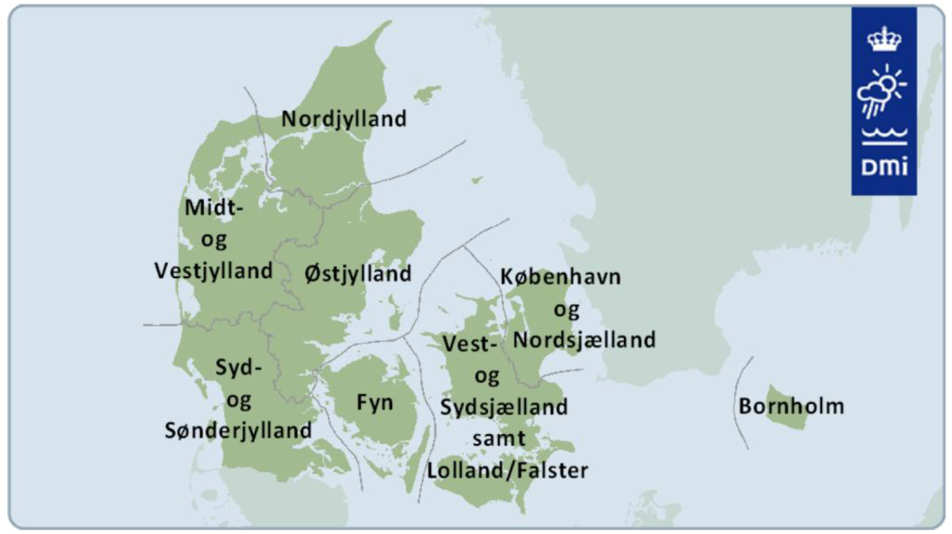
  13. Wang, P.W. Reference Values. In Technical Report 12-22-Reference Values: Hourly, Monthly and Yearly Values for Temperature, Relative Humidity, Wind Speed, Global Radiation and Precipitation for Regions and the Whole Country Denmark, in Period 2001–2010; Danish Meteorological Institute (DMI): Copenhagen, Denmark, 2013; pp. 6–8. (In Danish) [Google Scholar]
  14. Christensen, K. Calculation of Heat Demand. In Calculation of Gross Energy. Simplified Calculation. Teaching Notes; Department of Civil Engineering, Technical University of Denmark: Lyngby, Denmark, 2004; pp. 4–11. (In Danish) [Google Scholar]
  15. Kragh, J.; Wittchen, K.B. Calculation Assumptions. In Energy Demand of Danish Buildings in 2050. SBi 2010:56; Danish Building Research Institute: Copenhagen, Denmark, 2010; pp. 9–10. (In Danish) [Google Scholar]
  16. Tommerup, H.; Laustsen, J.B. Energy Saving Measures in Public Buildings. In Energy Savings in Buildings of Public Sector; Department of Civil Engineering, Technical University of Denmark: Lyngby, Denmark, 2008; pp. 10–39. (In Danish) [Google Scholar]
  17. Wittchen, K.B.; Kragh, J. Annex II—Display Sheets. In Danish Building Typologies. Participation in the TABULA Project. SBi 2012:01; Danish Building Research Institute: Copenhagen, Denmark, 2010; pp. 38–91. [Google Scholar]
  18. Wittchen, K.B.; Aggerholm, S. Calculation of building heating demand in EPIQR. Energy Build. 2000, 31, 137–141. [Google Scholar] [CrossRef]
  19. Wittchen, K.B.; Mortensen, L.; Holøs, S.B.; Björk, N.F.; Vares, S.; Malmqvist, T. Available Information in the Nordic Countries. Annex 1—Denmark. In Building Typologies in the Nordic Countries. Identification of Potential Energy Saving Measures. SBi 2012:04; Danish Building Research Institute: Copenhagen, Denmark, 2012; pp. 8–40. [Google Scholar]
  20. Bøhm, B.; Schrøder, F.; Bergsøe, N.C. Appendix; Domestic Hot Water. Measuring Consumption and Heat Losses from the Circulation Pipes. SBi 2009:10; Danish Building Research Institute: Copenhagen, Denmark, 2009; pp. 11–210. [Google Scholar]
  21. Bøhm, B. Production and distribution of domestic hot water in selected Danish apartment buildings and institutions. Analysis of consumption, energy efficiency and the significance for energy design requirements of buildings. Energy Convers. Manag. 2013, 67, 152–159. [Google Scholar] [CrossRef]
  22. Dyrelund, A.; Fafner, K.; Ulbjerg, F.; Rambøll Danmark; Aalborg University. Statistics and Prognosis. In Heat Plan for Denmark. Appendix Report; Rambøll and Aalborg University: Copenhagen, Denmark, 2010; pp. 173–186. (In Danish) [Google Scholar]
  23. Tommerup, H.M. Energy Saving Mesures in the Existing Buildings. In Energy Savings in Existing and New Buildings; Department of Civil Engineering, Technical University of Denmark: Lyngby, Denmark, 2004; pp. 17–43. (In Danish) [Google Scholar]
  24. Wittchen, K.B. Scenarios for Energy Savings. In Potentials for Energy Savings in Existing Buildings. SBi 2009:05; Danish Building Research Institute: Copenhagen, Denmark, 2009; pp. 17–34. (In Danish) [Google Scholar]
  25. Tommerup, H.M. Isolation of Building Envelope. Windows. In Energy Renovation Measures. Catalogue; Department of Civil Engineering, Technical University of Denmark: Lyngby, Denmark, 2010; pp. 10–15. (In Danish) [Google Scholar]
  26. Danish Energy Agency. Updated Sheet on Discount Rates, Lifetime and Reference for Guidelines for Socio-Economic Analyzes of Energy from April 2005 (Calculation Examples Revised July 2007). (In Danish)Available online: http://www.ens.dk/sites/ens.dk/files/info/tal-kort/fremskrivninger-analyser-modeller/samfundsoekonomiske-analysemetoder/notat_om_kalkulationsrenten_juni_2013.pdf (accessed on 27 October 2013).
  27. Ostergaard, P.A.; Mathiesen, B.V.; Moller, B.; Lund, H. A renewable energy scenario for Aalborg Municipality based on low-temperature geothermal heat, wind power and biomass. Energy 2010, 35, 4892–4901. [Google Scholar]
  28. Lund, H.; Mathiesen, B.V. Energy system analysis of 100% renewable energy systems—The case of Denmark in years 2030 and 2050. Energy Oxf. 2009, 34, 524–531. [Google Scholar] [CrossRef]
  29. Mathiesen, B.V.; Lund, H.; Norgaard, P. Integrated transport and renewable energy systems. Util. Policy 2008, 16, 107–116. [Google Scholar] [CrossRef]
  30. Gram-Hanssen, K. Existing buildings—Users, renovations and energy policy. Renew. Energy 2013, 61, 136–140. [Google Scholar] [CrossRef]
  31. Loulou, R.; Labriet, M. ETSAP-TIAM: The TIMES integrated assessment model Part I: Model structure. Comput. Manag. Sci. 2008, 5, 7–40. [Google Scholar] [CrossRef]
  32. Loulou, R. ETSAP-TTAM: The TIMES integrated assessment model Part II: Mathematical formulation. Comput. Manag. Sci. 2008, 5, 41–66. [Google Scholar] [CrossRef]
  33. Balyk, O.; Hedegaard, K. Energy system investment model incorporating heat pumps with thermal storage in buildings and buffer tanks. Energy 2013, 63, 356–365. [Google Scholar] [CrossRef]
  34. Zvingilaite, E. Modelling energy savings in the Danish building sector combined with internalisation of health related externalities in a heat and power system optimisation model. Energy Policy 2013, 55, 57–72. [Google Scholar] [CrossRef]

