1. Introduction
The environment affects agricultural production, via soils, weather, water availability, etc. and agriculture affects the environment via its impact locally on landscape, water, soil nutrition and biodiversity and more widely via its impact on climate change. Locating agriculture within its spatial environment is thus very important in making decisions by farmers, policy makers and other stakeholders.
Farm data availability is quite good, particularly in European countries as the collection of data within the Farm Accountancy Data Network (FADN) is a compulsory requirement of the EU Common Agriculture Policy. Within the EU, countries collect detailed farm data to understand the technical and financial performance of farms. The Farm Accountancy Data Network is designed to collect detailed farm management, financial and technical data representing the major agricultural enterprises. Its approach on collection and dissemination of data has always been by farm sector and enterprise type. The data, which is representative at the national level, is primarily used for comparing the financial performance of farms in different countries.
However, relatively limited information has been available at the spatially (NUTS 3 level only). Geo-referencing the data has the capacity to enable an improvement in the understanding of the interaction between environment and Agriculture. Kokic
et al. (2007) identify a number of advantages of geo-referencing farm data [
1].
The ability to ground truth models based on satellite data for natural resource management.
Improved measurement of greenhouse gas emissions such as carbon sequestration and emissions from agriculture.
An increased capacity to generate small area estimates that reflect the heterogeneity within and across landscapes.
An ability to undertake economic analysis of changes in land management practices based on the reliability of water supply and rainfall.
Improved methodologies for providing higher quality and more timely production forecasts through the capacity to analyse spectral signatures of crops and pastures using satellite imagery.
A better understanding of the economic impacts of pest and disease incursions on farms using finer resolution spatial data to improve the evaluation of post-incursion management options.
A reduction in the number of variables that need to be collected in surveys, resulting in reduced response burden.
Corbett (1996) argues that modelling within a GIS framework offers a mechanism to integrate the many scales of data developed in and for agricultural research, where an accurate spatial (and temporal) database enables the characterization of agro-ecosystems and is vital for efficient resource allocation in agricultural research. He notes that as agro-ecosystems are complex entities, a dynamic characterization requires both biophysical and socioeconomic data [
2].
Where farm survey data contains geo-referenced data, then it is technically straightforward to link environmental data to farm production data. Kokic
et al. (2007) describe a methodology for collecting spatial data. Many surveys, particularly in development situations, contain geo-referenced data [
3].
However, even where farm or postal address data is available, there are may be technical challenges in relation to geo-referencing farms. This is due to the fact that single grid references may not necessarily represent the spatial location of the farm, due to either multiple parcels or large size [
4]. There can also be challenges in relation data confidentiality, which prevent the sharing of data between the farm survey data collection agency and the researchers who hold spatial data.
Currently the knowledge of the spatial-environmental attributes of farms in survey data is quite poor as the spatial location of farms within these surveys is very limited. The only geographic information collected was the address of the correspondent. Delivering results on a sectoral basis satisfies the national FADN reporting requirements and also guarantees the confidentiality of the correspondents [
5]. Thus far these confidentiality objectives have limited the linkage of spatial-environmental data with these farm account and management data.
It is however intended that future EU-surveys such as the FADN and the Farm Structures Survey will be geo-referenced where the geo-referenced point will be the farmhouse [
6]. However, in order to be able to undertake farm productivity analyses as a function of environmental characteristics, it is useful to combine spatial and temporal data, in order to get both spatial and temporal variation. While in time, this data will become available, it would be useful now to look at alternative mechanisms to geo-reference historical farm survey data.
In this paper an address-matching methodology to geo-reference farm survey data is applied. Ireland is a good choice as a case study as the dominant farm systems are pasture based mainly animal systems and because the geo-referencing of addresses poses particular challenges outlined in
Section 2.1. As a pastoral system the local environment is particularly relevant to output. Agriculture in Ireland is also amongst the largest as a proportion of the size of the economy in the E.U. and thus the environmental impact is likely to be more important. The data used in this paper is the Irish variant of FADN, the Teagasc National Farm Survey (NFS) from 2008 [
7].
Since the establishment of the NFS methodology in the early 1970s, there have been major developments in Geo-Informatics such that the majority of agri-environmental data now has a spatial element and information is managed spatially with large geo-databases. In the last decade the use of explicit geo-spatial analysis within agri-economics has grown in importance [
8].
Retrospectively spatially-enabling the NFS would allow the records collected to be used more easily within this new geospatial environment. Allotting each farm correspondent in the NFS with a geographic coordinate would allow for the allocating of data to each farm from geo-spatial or map sources [
9] (for example, calculating actual road distance to the nearest mart for all beef farms in the NFS). With a Geo-spatially enabled NFS historical weather records can be ascribed to each farm or see how decisions year-on-year are influenced by weather. There have been attempts in Europe to downscale the published national and regional accounts to provide an ersatz spatial FADN [
10], this paper is the first example of a national farm accounting system to be fully geo-referenced and analysed.
An earlier Teagasc programme had success matching addresses to Districts and linking farm soil samples to ED maps via addresses attached to sample [
11]. Also there are a number a number of firms in Ireland that offer matching to the national address database, the GeoDirectory, as a service (see
Section 3.1). However while these services are available for sale their algorithms are not available for research purposes. In this paper the geo-referencing of addresses specifically within the Irish Farm Accountancy Data Network is described and the particular challenges the of the Irish address system are outlined.
Applying this methodology has a number of challenges because Ireland does not have a system of post (zip) codes. In addition there are complications in relation to place names which may be in English or Irish or a combination, often with non-harmonised spellings and with non-unique place names. The conventional SQL based methodology shown in this paper overcomes these difficulties.
The primary objective of the NFS is to provide a nationally representative picture of farm outputs and outcomes for different farming systems it is not intended to be geographically representative. As a result the survey may not represent all agri-climatic zones in the country and may not necessarily be representative spatially of the distribution of environment x farm system. Within the paper the geographic representativity of the data with respect to climate is assessed. This is important; FADN data is often used as the basis for studies of the impact of future climate change on agriculture [
12]. If the FADN sample is significantly different environmentally than the average farm in any given national report (with Ireland as the example in this paper), these predictions of climate change on farm production could be skewed at a national scale (its less likely to have an impact when analysed at a regional European scale [
13]).
2. Technical Challenges
2.1. Geo-Referencing
There is a significant challenge in geo-referencing farm survey data in Ireland. Firstly, the country does not have postcodes (unlike most other European states) and at the same time for linguistic, cultural and measurement reasons there is a significant degree of uncertainty in relation to place names with frequent differences in spelling and occasional duplication of the same name. Future Geo-coding of FADN data across Europe is likely to be based upon parcel identification reducing the dependence on address matching.
The history of Irish toponymy is a complicated story of local place-names surviving against imposition of standards by different authorities. The official allocation or recognition of place names (vested in An Coimisiún Logainmneacha) is based upon the historical development of administrative units [
14]. In practice Irish addresses have a wide range of forms. In rural Ireland they tend to conform to the following type:
As locality/townlands contain a multitude of households; if the household does not have a street number (as is the case in most rural areas) then the address given does not uniquely identify a building/home in rural Ireland. In practice the successful operation of the postal service relies upon the knowledge of the local postal worker regarding the names of occupants.
The “official” registry of addresses maintained by the postal service is the GeoDirectory, which attempts to impose a structure on addresses. Each system uses the Central Statistical Office/Ordnance Survey of Ireland address system, it is in four parts:
Building no./street/locality, townland/town, town/county, county
For example: Teagasc Research Centre, Malahide Rd, Kinsealy, Co. Dublin
However examples of common alternate address forms for the same location include:
Teagasc, Kinsealy, Malahide, Co. Dublin
Teagasc, Kinsaley, Malahide, Co. Dublin
Teagasc, Mullach Ide, Baile Atha Cliath (Irish version)
All of these addresses are “official” and correct. On top of these official variations there are accidental misspellings, colloquial alternative spellings and reversals. With that proviso a more formalised addressing system would be useful and the GeoDirectory attempted to provide this.
The Teagasc National Farm Survey (NFS) used in this study uses the same address coding as the GeoDirectory, which makes the task relatively easier. Also, as the use of Irish names of localities more commonly referred to in English in the collection of the NFS was not widespread and therefore the alternate automation of English/Irish place names was not necessary.
In order to link local environmental data to the financial data in the NFS, a challenge therefore in this paper is to identify the location of addresses in the NFS to data points in the GeoDirectory.
2.2. Geographic Sampling
Once addresses are identified, there remain a number of potential sources of geographic sample issues—the tendency of the NFS to sample in particular regions rather than randomly across the country. These include a number of reasons.
Firstly, agriculture is not the main land use across all of the physical space. Other land use and land cover include buildings, roadways, water, land areas not suitable for agriculture such as higher altitude, bog and poor land quality, etc.
A second reason is that the farm survey data utilised does not optimise its sample geographically. Rather the objective of the sampling is to maximise the volume of output. It also ignores certain types of farms such as smaller farms, and farms with particular types of enterprise such as pig, poultry and horticulture farms. If the spatial pattern of the types of farms is spatially non-random, then one will observe a geographic bias.
A third potential reason may result from the spatial pattern of data collectors, which, although spatially distributed is spatially non-random, which may result in non-response bias due to time taken to reach destinations.
A challenge therefore is to compare the geographic distribution of farms in the survey versus farms in the country.
4. Methodology
There are three parts to the problem of spatially enabling the farm survey for allocation of environmental attributes:
Matching addresses in the NFS to possible addresses in the GD.
Allocating a geographic point that represents the matched GD addresses that deals with the one-to-many matching possibilities and retains an element of confidentiality in the data.
Ascribing a representative sample of the environmental attribute to the point.
4.1. Address Matching
The first task required is to match the NFS addresses to the GD addresses and resulting GIS coordinates. As the order of complexity is quite high, the algorithm was tested initially on a pilot sample of 51 addresses. These were examined manually and matched against the GD. The 51 addresses were matched using Access SQL. In order to cope with the alternate spellings and truncated address already identified, the scripts were written to give a positive match against first (initial) and last two letters of a locality and townland or to match the first five letters or the last five letters of the locality to the townland—matching always against county. The number five was used to allow bally* names (bally is an anglicised version of baile, the Irish word for town) to be identified and *stown name to be identified (town is possessive in an Irish placename context and thus is often preceded by “s”, e.g., Abbotstown).
This resulted in the automatic matching of 44 of the 51 NFS records—three more records could be manually matched (the names were very different but recognisable) and the remaining four points are manually matched against the most likely address(s). The NFS records were matched to GD clusters of addresses ranging from 1 to 45 houses.
After this pilot, we proceeded to the geo-enabling of the whole of the 2007 NFS address database. The full list supplied contained 1,350 records. Detailed examination of this list revealed a number of data capture issues, such as different formats for the county name: Dublin or Co Dublin or Co. Dublin. These issues and others could have been dealt with in SQL but it was decided to do a preliminary clean of the input addresses in MS Excel. Rules were refined and added to. A common source of confusion in this set was the swapping of address elements. Thus the rules had to be expanded to include these permutations. An extra set of rules that matched against the first two letters of the first three address elements was also introduced.
A detailed examination of a subset of the unmatched set showed that the sources of confusion were many and that to incorporate these as SQL rules and run on the entire database would take longer than manual checking. Therefore the remaining names were checked and matched manually. Even with manual matching 85 addressed could not be identified with any confidence and have not been included in subsequent analysis.
4.2. Geo-Locating
The majority of NFS addresses match to multiple building points thus a method to ascribe one point to the NFS address, with the assumption that in a one-to-many match one of the houses is the actual farm house, is needed.
Because of the inherent resolution in the environmental datasets, there is no need for accuracy greater than 1km as the climate models have a 1 km cell size and a point to bear in mind is that the GD point is allocated to the
farmhouse not the farm, see the discussion in
Section 1.
When trying to assess the environmental drivers of farm performance for an individual farm then ascribing its location to a point is a poor choice- farms are areas that vary enormously even within themselves. However, for this study, investigating the spatial distribution of farms nationally, points are adequate.
As outlined above there are potentially many possible households that can represent the NFS address for the reasons given above. For our purposes the geographic centre of each cluster is chosen as the representative location.
4.3. Geographical Sampling
One of the objectives of this paper is to test the geographical sample of the farm survey data. In other words; to see if the spatial spread of sampled farms is equivalent to the spatial spread of actual farms. One potential way of doing this is to break the country up into grids and to test the distribution of farms across grids relative to the true distribution of farm addresses. However as the survey is a sample of about 1%, this method is not feasible due to the scarcity of the data.
An alternative method of assessing the any trend is to consider a uniformly distributed population across a square or parallelogram, as is the case with coordinates expressed in the Irish National Grid. If the x coordinates are plotted against the y coordinates in rank order, then in an evenly spread population, the outcome is a straight diagonal line plot. In this case a graphical illustration of trends for an alternative population would be a deviation from this line (see
Section 5.2).
Thus the spatial coordinates x and y are treated as matched sample pairs and plotted as the equivalent of p-p diagrams, i.e., in practice, the x coordinates and the y coordinates of the sample farms are sorted independently minimum to maximum and the ranked paired up and plotted.
However the terrestrial landmass of the country is only a subset of the national grid and is an irregular shape and is thus not a parallelogram. Therefore a plot matched ranked pair plot of random points on land is not quite a straight line. Nevertheless the geographical trends can still be observed if there is a deviation from this line. Comparing the plot for sampled farms, the distance between the two plots indicates the geographical trends.
This approach has parallels with non-parametric ranked tests of difference. Compare with the Kolmogorov-Smirnov test for examining if two samples are similar, where the data points are combined and ranked and the maximum cumulative difference is calculated.
An advantage of this method is that it can be used to compare distributions with different underlying sizes. So for example there are about 120,000 farms in the population, but only 1,350 in our sample. Nevertheless, the x and y coordinates can be plotted and compared against each other. At present we have not developed a method to test the statistical properties of this comparison and so are not in a position to test the statistical significance of the difference.
5. Results
The degree of impression, as outlined below, within the matching algorithm is less than the resolution of the climate data (1 km Square cells) and thus it can be used for our purpose- testing the geographic NFS sample with respect to agri-climatic variables. In this section spatial-environmental representativity is tested. To do this the spatial pattern of geo-referenced NFS points are compared against national geographic and environmental datasets.
5.1. Assessment of Geo-Referencing
Utilising the method described in
Section 4, the pilot analysis is extended, running the rules sequentially; matching 1,350 addresses to a database of over 1.5 million resulting in approximately 1,000 positive matches. These positive matches sometimes included false positives but these are easy to eliminate by hand.
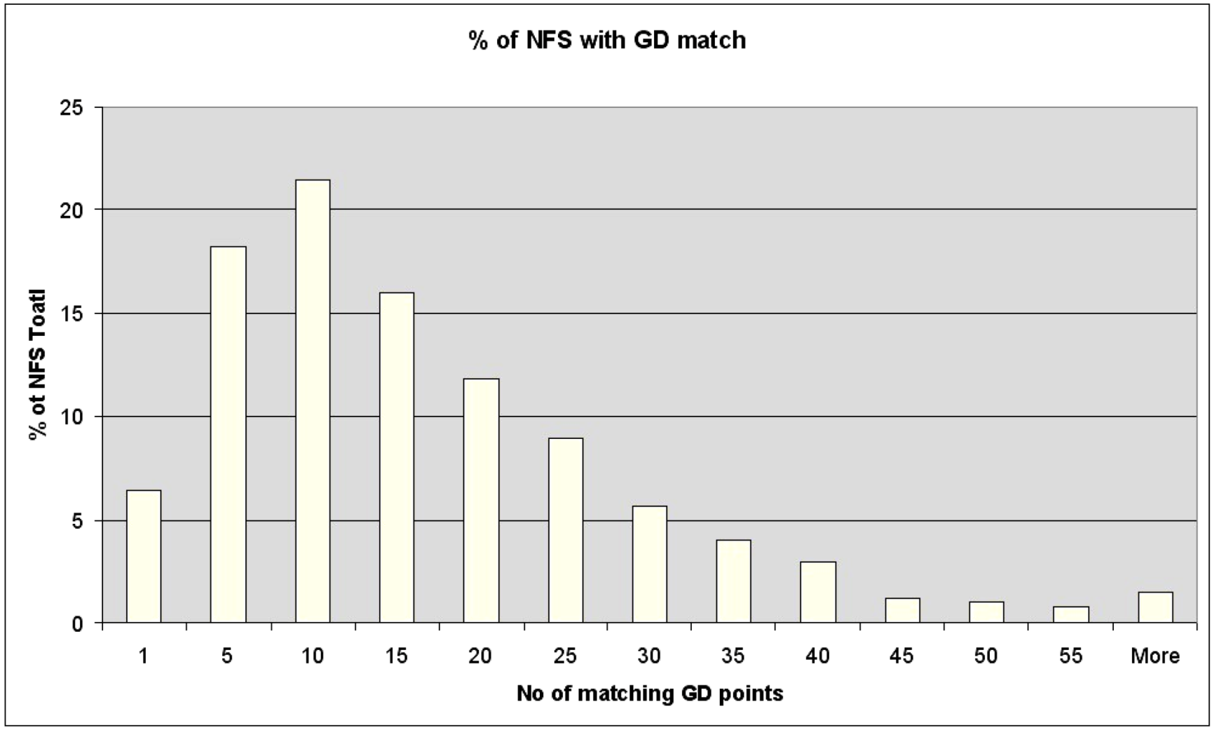
In
Figure 2, are reported the percentage of NFS addresses that automatically match with a given number of buildings in the GD. We can see that only 6% of NFS addresses match on a one-to-one basis with a GD building, the rest match against a range of numbers of buildings, with NFS addresses matching to 10 GD buildings on average. It should be noted that this is not an “error” as all 10 of the buildings in the GD have exactly the same address.
Figure 2.
Frequency histogram percentage of the National Farm Survey (NFS) addresses that match to a cluster of houses of a given size.
Figure 2.
Frequency histogram percentage of the National Farm Survey (NFS) addresses that match to a cluster of houses of a given size.
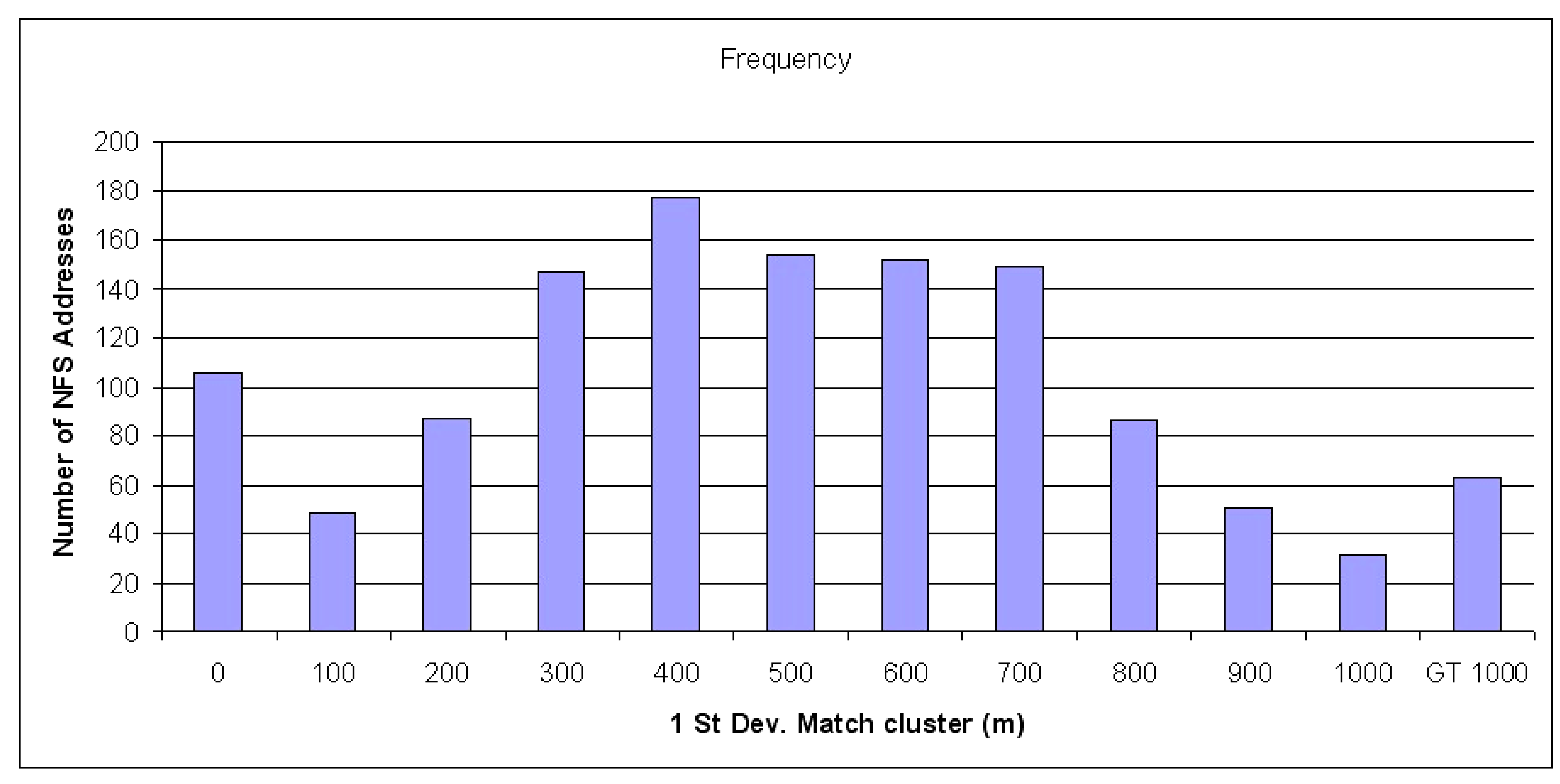
A frequency histogram in
Figure 3 shows the distribution of 1 standard deviation cluster sizes. The average cluster of GD buildings associated with a NFS address has a standard deviation from the mean of 475 m. This implies that the automatic geo-coding method described here has an inherent precision of 1 km. This is adequate for environmental/climate studies being undertaken.
Figure 3.
Frequency histogram showing the size of 1 standard deviation from the geographic mean of each building cluster.
Figure 3.
Frequency histogram showing the size of 1 standard deviation from the geographic mean of each building cluster.
Note: A value of zero means that the NFS address was matched to a unique address in the GD.
5.2. Assessment of Geographical Sampling
To examine the geographic distribution of the NFS farms, we compare the spatial pattern of NFS farms with the actual distribution of farms, that of non-NFS farms. The data was created in the following way:
A national geographic distribution was established by randomly selecting 1,000 points across the Republic of Ireland (this is the NATional dataset).
This is also done for the other two data sets (the NFS points and the NON-nfs farming control set).
Address points for non NFS farms was created by taking data from the CSO Census of Agriculture 2000 at the district level, showing number of farmers, and average size of farm have been used in testing the spatial characteristics of the NFS (CSO, 2002). Centroids for all Districts were calculated. All the districts with NFS points within them (~900) were eliminated and so too were all the districts that, according to the CSO Census of Agriculture 2000, had no farmers. This left ~1,900 points (the district centroids) to act as dummy farms—the non-nfs set. This sample set is geographically weighted but is not weighted to population of farmers.
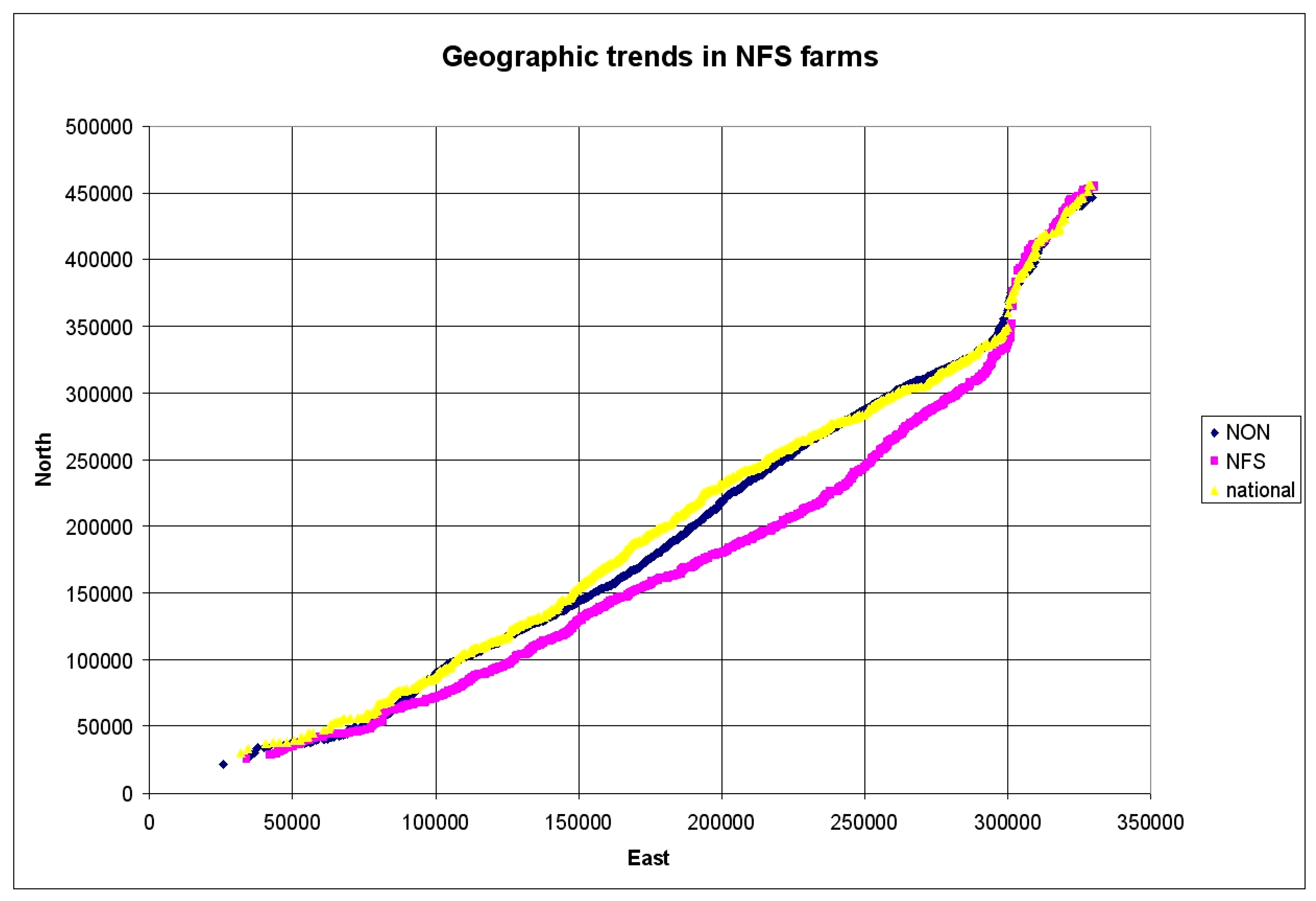
An examination of possible
geographic sample in
Figure 4 indicates differences between the NFS set, the non nfs and a national set. The plot is created as outlined in
Section 4 above—the x and y coordinates of the different samples are ranked independently lowest to highest—than corresponding ranked pair are plotted
Figure 4.
Spatial distribution of National point set, NFS point set and NON point set.
Figure 4.
Spatial distribution of National point set, NFS point set and NON point set.
Note: The axes are ING coordinates in x and y. In the ING the bottom left of the National Grid is 0,0 and the value increases to the East and to the North. Thus the ‘kink’ in the plot beyond 350,000N and 30,000E is caused by the lack of samples in Northern Ireland.
This plot has to be interpreted carefully. As can be seen the National random set (yellow) has a very similar spatial distribution to the NON NFS farm points (blue). The pink NFS points are distinctly different. The plot is read as increasing east left to right and increasing North bottom to top. So the kink in the top right hand quadrant is a caused by the lack of points in Northern Ireland and is interpreted as above 350,000N the points sampled are tending westward (County Donegal). This should help in interpreting the NFS data points. We can see, as the pink bulges below the national trend, that the GNFS points trend both more easterly and southerly than the national and non-nfs sets.
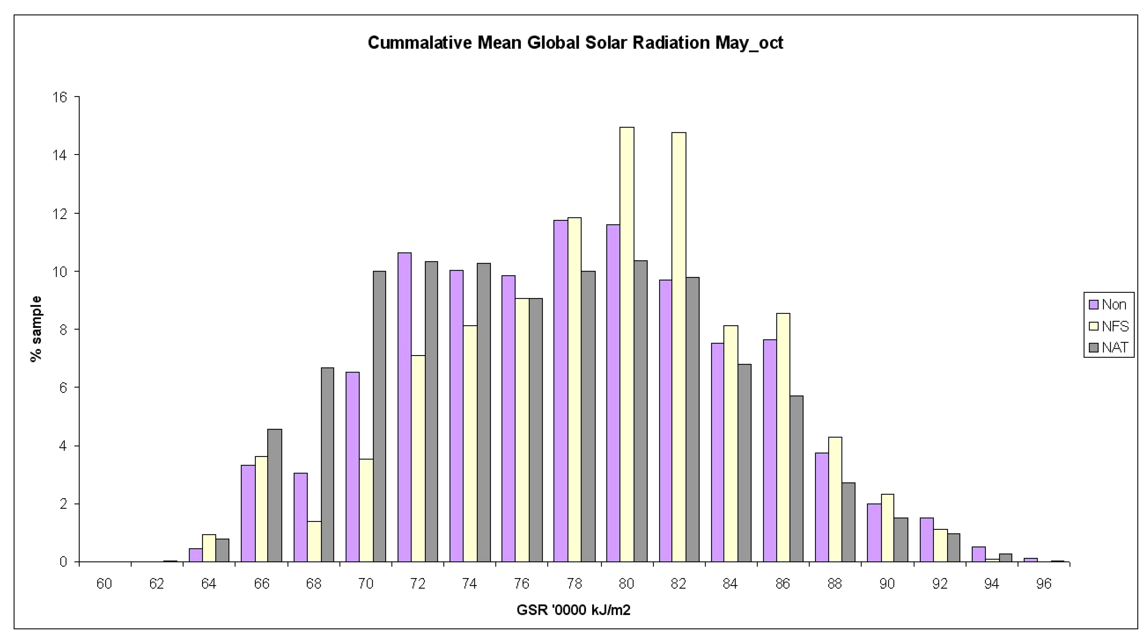
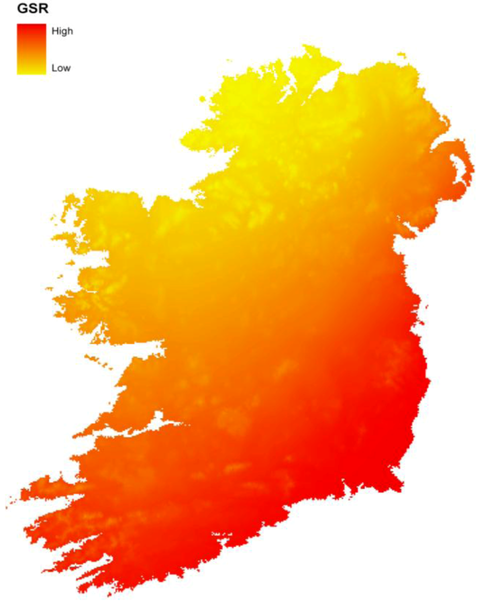
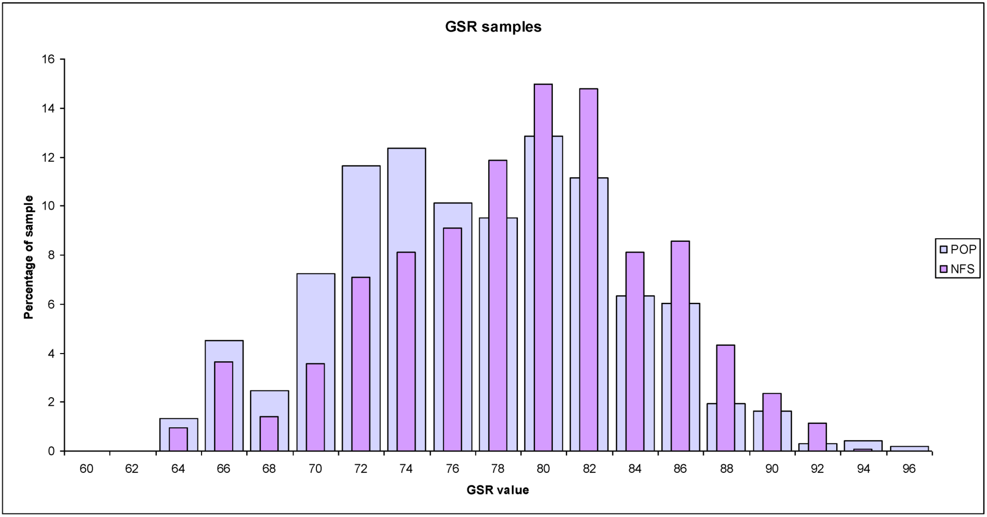
In order to test the spatial-environmental representativity of the survey, we link our data points to from the NFS-GD match to environmental data. A test on using the NFS points to extract climate information was also carried out. Climate surfaces as outlined above were used. We take from an interpolated surface based on climate station trend data against elevation data. For each NFS the value for the coincident 1 km cell was attributed to the NFS point as the levels of precision are the same. The actual values are unimportant in this case we are interested in the trend; high levels of GSR in the South East and lower levels in the North West of the country.
Figure 5 shows the distribution of values of the annual average accumulated summer GSR for the three test sets, national, NON-NFS and NFS. In this case the national set is the values for all the grid cells in the ROI map (every fourth value, 5,240 in total).
Figure 5.
The Distribution of Global Solar Radiation.
Figure 5.
The Distribution of Global Solar Radiation.
Note: Frequency histogram showing distribution of Global Solar Radiation values associated geographically with points from a NATional set, NON NFS set and NFS farm set.
We can see that the distribution of the non-NFS dummy farms nearly matches that of the national distribution. The Distribution of the NFS set is quite different, skewing toward higher values.
Is the skewing significant? The samples here are very large compared to the national sample (1,260 to 5,200) and thus tests based on the mean could give an erroneous impression. Examining the plots draws us to the hypothesis that the standard distribution of GSR values in the NFS sample is significantly different to the national set. To test, a two-sided F-Test was applied to both the National vs. Non NFS samples sets and the National vs. NFS sample sets.
For the NON-NFSpoints (
Table 1): Formally the null hypothesis is σ
NAT = σ
NON and the alternate hypothesis σ
NAT ≠ σ
NON.
Table 1.
Summary two sided F-test for National/NON-NFS sets.
Table 1.
Summary two sided F-test for National/NON-NFS sets.
| | Nat | Non |
|---|
| Mean | 75.74340295 | 77.08326 |
| Variance | 41.21613302 | 39.67419 |
| Observations | 5246 | 1898 |
| Df | 5245 | 1897 |
| F | 1.038865058 | |
| P(F ≤ f) one-tail | 0.318 | |
| F Critical one-tail | 1.077814282 | |
The F value (1.038) is less than the critical f value (1.077 at 95% confidence limit) therefore the null hypothesis is not rejected and we can say the standard deviation of both is the same. Thus, the NON-NFS sample set is a reliable sample of the national climate data examined.
For the NFS points (
Table 2): Formally the null hypothesis is σ
NAT = σ
NFS and the alternate hypothesis σ
NAT ≠ σ
NFS.
Table 2.
Summary two sided F-test for National/NFS sets.
Table 2.
Summary two sided F-test for National/NFS sets.
| | Nat | Nfs |
|---|
| Mean | 75.7434 | 78.03912656 |
| Variance | 41.21613 | 35.11558417 |
| Observations | 5246 | 1156 |
| Df | 5245 | 1155 |
| F | 1.173728 | |
| P(F ≤ f) one-tail | 0.000638 | |
| F Critical one-tail | 1.095755 | |
In this case the F value (1.173) is greater than the critical value (1.09 at 95% confidence) therefore the Null hypothesis is rejected in favour of the alternate, that the standard deviation of the NFS sample is significantly different to national sample.
A non-parametric test was applied to test the hypothesis that, of the two samples, the NFS climate variable contains significantly higher values than the national sample. The Mann-Whitney U test makes no assumptions about the distribution of the data (other than the null hypothesis that the distributions are the same) and in the test the two samples are ranked and the ranking compared. The U statistic is a measure of how different the ranks are. In the U test the null hypothesis is that the samples are the same—the results of the application of this test is that NFS sample of GSR is significantly different from the national set with P < 0.001 (two sided test).
Difference in farm characteristics between the NFS and the non-NFS datasets are also evident, by looking at farm characteristics of the Districts with NFS points and compare to those without. Average farm size is covariant with many other economic variables and thus was selected as a test variable.
Figure 6 shows the frequency histogram of average farm size within NFS Districts and NON NFS Farm Districts. As we can see the distributions are similar (though the NFS has a slight skew toward larger farms). This is not unexpected as the selection of farms is matched against CSO census data.
Figure 6.
Frequency histogram of average farm size within NFS Districts and NON NFS Districts.
Figure 6.
Frequency histogram of average farm size within NFS Districts and NON NFS Districts.
8. Conclusion
In this paper, farm households in the Irish sample of the Farm Accountancy Data Network (FADN) were geo-referenced. Testing for statistical differences in agri-climatic variables as sampled by the NFS, we note a significant difference between the sample and the underlying distribution.
The National Farm Survey, as part of FADN, is designed to accurately represent farm systems. The geo-referencing of farm survey data enables future analyses of the distribution between farm output and cost data and environmental attributes. However, as we have shown here that, in Ireland’s case, it does not represent farm geography fully and the data may limit some analyses where particular combinations of environmental variables and farm variables are missing due to the nature of the sample. This could have implications if FADN data are used at a national level to predict the production and agri-economic impacts under different climate change scenarios.
This issue could also impact on those downscaling techniques that rely on establishing spatial covariance of regional FDAN data with regional spatial land use and environmental data if the model assumes that the FADN sample is a representative sample of the various agri-environmental geographies in the region.
As the European FADN system moves toward introducing a geospatial element to its reporting it may be necessary to adapt the current sampling strategies to ensure that the sample chosen equally represents geography (both European and national) as well systems performance. It cannot be assumed that a 1% sample of European farms systems will represent the full environmental geography of European agriculture. Importantly retrospective address matching of historical FADN survey data will ensure that the existing surveys will be fully compatible with future surveys that contain detailed geographic information.


