
A Novel Heuristic Emergency Path Planning Method Based on Vector Grid Map
by
Bowen Yang
1, 
Jin Yan
2,
Zhi Cai
1,
Zhiming Ding
1,2,3,*,
Dongze Li
1,
Yang Cao
4 and
Limin Guo
1 1
College of Computer Science, Beijing University of Technology, Beijing 100124, China
2
Institute of Software, Chinese Academy of Sciences, Beijing 100190, China
3
Beijing Key Laboratory on Integration and Analysis of Large-Scale Stream Data, Chinese Academy of Sciences, Beijing 100144, China
4
School of Information, Beijing Wuzi University, Beijing 101149, China
*
Author to whom correspondence should be addressed.
ISPRS Int. J. Geo-Inf. 2021, 10(6), 370; https://doi.org/10.3390/ijgi10060370
Submission received: 3 April 2021
/
Revised: 16 May 2021
/
Accepted: 26 May 2021
/
Published: 31 May 2021
Abstract
:Emergency path planning technology is one of the research hotspots of intelligent transportation systems. Due to the complexity of urban road networks and congested road conditions, emergency path planning is very difficult. Road congestion caused by urban emergencies directly affects the original road network structure. In this way, the static weight of the original road network is no longer suitable as the basis for path recommendation. To handle the dynamic situational road network, an equidistant grid emergency path planning framework will be designed. A novel situation grid road network model, based on situation information, is proposed and applied to an equidistant grid emergency path planning framework. A situational grid heuristic search will be proposed methodology based on this model, which can be used to detect the vehicles passing around the congestion area grid and the road to the destination in the shortest time. In the path planning methodology, a grid inspired search strategy based on quaternion function is included, which can make the algorithm converge to the target grid quickly. Three graph acceleration algorithms are proposed to improve the search efficiency of path planning algorithm. Finally, this paper will set up three experiments to verify our proposed method.
1. Introduction
In recent years, with the urban road network becoming more and more busy, emergency detour path planning is becoming more important overtime. Some road congestion often occurs on urban roads, in the morning and evening rush hours in the city, especially, road congestion is more serious. As a result of this situation, several studies have been conducted about how to successfully make cars avoid congested areas to ensure that the vehicle can travel to its original destination in a shortest time. Therefore, this path provides a detour for vehicles an emergency path [1,2].
At present, some researchers have proposed related evacuation models and models of evacuation congestion in this research direction [3,4,5,6,7]. The existing researches about path planning mainly focus on the dynamic path planning of static road networks. Kim et al. [8] proposed an evacuation route planning (ERP) model using the spatial structure of the road network to minimize computing time. The other kind is an emergency path planning system based on traditional scenes. Khalid et al. proposed that using an immune-based approach to solve the dynamic path planning problem [9]. This method reduces the computational complexity and optimal solution generation of the meta-heuristic method, and the heuristic method adopts the immune-based comprehensive evacuation planning (iEvaP+) method, which is dynamic. Zhang et al. [10] presented a collaborative situation model of people and vehicles. This model is a comprehensive linear model of the optimal design for a large number of mixed flow involve pedestrians and vehicles in the detour area.
Other studies focus on the short-term and long-term predictions of the road traffic [11]. Li et al. [12] studied an efficient method for spatio-temporal neural structure search-automatic search. This method is mainly to update the spatio-temporal correlation of each convolutional layer and the method of treaty learning between layers. Dai et al. [13] presented a hybrid spatio-temporal graph convolutional network (H-STGCN), which is able to “deduce” future travel times by using incoming traffic data. For example, when the information is disturbed or missing, this method can effectively predict the existing road traffic flow with reference to context information. Lin et al. [14] proposed that a dynamic switch-attention network (DSAN) with a novel multi-space attention (MSA) mechanism that measures the correlations between inputs and outputs explicitly. This method can effectively filter the noise to reduce the error of prediction. The method can effectively predict the traffic flow in the short-term and long-term.
However, all the above methods train and calculate the historical data. In the emergency scenario, the existing traffic flow cannot be predicted effectively through the historical data. The reason is that the randomness in the emergency scenario is relatively large, so the probability of the occurrence of emergency events in a certain road area of the city cannot be calculated through probability. For example, Figure 1 shows that when urban vehicles encounter road congestion, they need to make detours in advance. Therefore, the challenge of this paper is focused on how to give top-k detour paths on the road network diagram with situational dynamics, so that the vehicle can bypass the emergency area and drive to the destination in the shortest time.
To address these issues, an equidistant grid emergency path planning (EGEPP) framework will be introduced in this paper. This framework is an improvement of the grid map emergency path planning (GMEPP) framework proposed in our previous work [15]. The GEMPP framework is mainly applied to the evacuation path planning of emergency paths and does not consider the planning of detour paths. Therefore, we mainly rely on the road network speed and road capacity as the basis for path selection and grid selection in the EGEPP framework. What needs to be noticed here is the characteristics of the dynamic road network because the emergency time starts at random, but the development of the process is that the traffic flow in the vicinity gradually decreases over time, which means that the number of vehicles in the congested area is consistent with normal distribution [16].
Based on this situation, a novel situational grid road network model (SGRN) will be designed, the model maps the road network with the spatial-temporal characteristics of the situation into a dynamic road network diagram that changes with time. Then a situational grid heuristic search algorithm (SGHS*) based on SGRN will be introduced. This methodology will use the sum of the time consumption function, and a time heuristic function determines the path selection. It also contains a pruning strategy based on a dynamic road network. Finally, we propose a road network acceleration algorithm based on the situation grid to optimize the query path. In short, the contributions of this study are summarized below:
- (1)
- This paper introduce a situational grid road network model under the situation of the emergency called SGRN model;
- (2)
- A novel method called dynamic grid PageRank (DGPR) can sort all grids according to the traffic capacity of the road network at the current moment and assign different grade values to each grid;
- (3)
- A SGHS* algorithm will be introduced with a spatial-temporal dynamic map, this method plans the detour path according to the sorted grids and composes the overall planning result by planning the two parts between the grids. According to the SGHS* path planning algorithm, a pruning strategy based on time characteristics is proposed to ensure that the path results given in a given time window make the vehicle travel the least time-consuming;
- (4)
- Finally, three road network acceleration algorithm situational contraction hierarchies (SCH), situational grid contraction hierarchies (SGCH) and a situational grid multiple reverse contraction hierarchies (SGMRCH) will be is proposed based on situation grid. There are three methods can establish a road network contraction Hashtable and change the relationship between the shortcuts added after the road network vertices and the original edges [17].
The rest of this paper is organized as follows. In Section 2 introduces the primary related work. In Section 3, a new model for emergency path planning is presented. Section 4 introduces details of grid sorting DGPR algorithm based on grid map. Section 5 describes a detour path query SGHS* based on grid map and pruning is performed according to a given time window . In Section 6, three acceleration considering dynamic road network circumstances will be introduced based on situational grid map. In Section 7 presents the experiment to verify the efficiency of EGEPP is introduced. The conclusion of this paper is in Section 8.
2. The Related Worked
The is a search in the state space, evaluating each search position, which can be obtained in a single search for the best position, and searching from a given origin to the target. This can omit a lot of unnecessary searches and improve efficiency. Valuation of location is very important in heuristic search. Different valuations used can have different effects. Heuristic search has several advantages: (1) The search from the current location to the target, and the downward search ensures that the solution obtained in the same hierarchy is optimal. This eliminates a lot of unnecessary search paths. (2) In the process of searching the target vertex, the algorithm can converge quickly if the heuristic function is designed properly. (3) In a certain search area, the breadth of search vertices is guaranteed, i.e., as much information of search nodes as possible is obtained.
A* algorithm is good at solving the problem of the static path in the shortest distance and is different from the Dijkstra algorithm and Floyd algorithm, this algorithm combines advantages of breadth-first search (BFS) and Dijkstra algorithm [18]: in the heuristic search at the same time, enhance the efficiency of the algorithm can guarantee to find an optimal path (based on the evaluation function, such as the Manhattan distance, Euclidean distance), Floyd algorithm [19] using more scenes in robot path planning, game programming, satellite path search, and other fields.
Singh et al. [20] studied a real-time A* (RTA*) algorithm was used for online search and optimization. The minimum energy consumption function is established. This method realizes the navigation of mobile robots in static obstacles and generates the path of minimum energy consumption by constraining the robot to move in the optimal direction. Khalidi et al. [5,21,22] proposed a path planning method T* based on heuristic time dynamic monitoring. The T* algorithm does not focus on path optimality, but on reducing the computation time of finding the path. For example, sampling-based linear temporal logic (LTL) motion planning algorithms can effectively compute trajectories in a continuous state space, but do not guarantee optimality. Bhatia et al. [23] proposed a path planning technology based on multiple layers. The advantage of this method is to reduce the search space as much as possible in the path planning by constructing discrete trajectory, so as to reduce the time of path planning in turn and improve the search efficiency. Mashayekhi et al. [24] studied an rapidly-exploring random tree based A* (RRT*) algorithm for the unmanned vehicle, the algorithm increases the heuristic strategy and greedy thought, on the original rapidly-exploring random tree (RRT) algorithm [25], the algorithm improved the way of the parent vertex selection, the cost function is used to select minimum cost within the territory of expanding vertex to the parent vertex, at the same time, after each iteration will reconnect the existing vertex in the tree, so that the complexity of the calculation and progressive optimal solution.
Other studies have also proposed strategies based on breadth search graphs. Guo et al. [26] proposed the Dijkstra algorithm path planning strategy based on the dynamic road network, and analyzed the effect of the algorithm under the conditions of the shortest time, shortest distance, and least fuel consumption through simulation experiments, which ensured that reasonable vehicles are provided in cities with growing population path planning strategy. Fink et al. [18] adopted a multi-objective variant of Dijkstra algorithm based on terrain data to achieve the overall optimal traversal in the 3D surface. The gained results were employed in the global rover horizontal optimization planner (GRHOP) automation system to quickly and accurately set up optimized routes for multiple constraints at the same time. Souza et al. [27] applied the Dijkstra’s method to tree diagram analysis, using mining blocks as nodes of the tree for analysis, and used to calculate the lowest cost route to transport mining blocks to their destination. The transportation cost was rejected in the arc of the graph, and it could use Euclidean distance or transportation time to calculate the minimum path.
There are two points to consider in the case of emergency path planning on urban roads. One is dynamic path planning based on the situational road network. Situational information is first of all a dynamic variable that changes over time. At different times, the values of the situational variables change based on the current relevant information. The second factor is path planning in the step search (from the current node to other nodes search process), consider joining the breadth search node strategy, meet the conditions as far as possible to the needs of traffic congestion areas, make the vehicle road traffic conditions better. Table 1 shows the main parameters mentioned in this article. Table 2 presents the abbreviations and full names of the methods mentioned in this paper.
3. Two New Models Based on Emergency Path Planning
This section will describe two models; the spatial-temporal road network model and the situational grid road network model. Both models are improved based on the graph structure pattern. In particular, the SGRN model improves the original graph structure model to a model that uses the characteristics of regional roads to represent road weights.
3.1. Spatial-Temporal Road Network Model
A spatial-temporal graph based intersection can be represented as a directed Graph G = , where V is a set of intersections and is a set of ordered pairs of vertices and indicate that there is a path between to , and . Noted that the direction of each path is a vector and the time at point is ahead of time. One path means vehicles start form a source point and arrive at point , with a weight w:= defined as time cost for a pair of intersection i to j, w is a non-negative number is all lengths are positive.
It is emphasized that the time represents the average time of the vehicle passing through the road of two intersections, and the value of is a function represented as , which is not fixed and stands for the length of the road, S is the average speed of the vehicle. The speed of the road network S at the query time window is taken into consideration in the path planning method. The purpose of is to ensure the optimal path for users at this moment, because S of the road has a different value at different times.
3.2. A Situational Grid Road Network Model
A situational grid map is modeled as a = <, , ()>, where is the whole city map in gird × and represents ID in the map (the value of will be given in details in the experiment section), indicates a ratio of the number of intersections in the grid to the number of intersections in other grids. The value of this ratio will be considered as the commuting ability of the grid. The sorting algorithm will adopt a PageRank based grid sorting algorithm GPR (the implementation of the algorithm will be described in detail in Section 4). stands for all the vertices in the grid, the more intersections in a grid, the stronger the grid’s ability to communicate to other grids, the other is an out-degree set that contains all the vertices in each grid.
The grid map divides the entire map into several sub-maps, . There will be several intersections and roads in each grid, and these factors will be taken into account when assigning values to the grid. After dividing the map into multiple areas, the framework can assign values to each area according to the setting of parameters. These values provide an important basis for evacuation path planning. The change of these values exactly reflects the weight change of the region, and at the same time provides a reliable basis in theory, which guarantees that the method will quantify intersections and roads into computable weight problems when the algorithm search for paths later. This is exactly the advantage of doing a path search on a grid map. It is worth noting here that the irregular shape of the city map causes some grids to contain no intersection or road after our grid, so these grids ID will be deleted from the data during preprocessing.
In this paper, the means that the road network is a real-time change of road conditions commonly known [28,29]. The congestion level of urban road networks generally changes with the change of time, meanwhile, the congestion level at the same time is also different due to regional differences. This kind of changing road network condition affect by time and geographical location is called the situation road network with spatial-temporal characteristics. The reason that the situation information on the road network should be considered is that the congestion area is not fixed, and the degree of congestion is also different (In this paper, the road congestion will be expressed through the speed of the road network, so it is no longer relevant to the congestion).
4. Equidistant Dynamic Grid Map Based on Situational Road Network
In this section, a dynamic approach to the grid road network with equal spacing will be introduced. An equal-spacing grid means mapping the entire road network into two-dimensional plane coordinates and segmenting the road network as a whole. Figure 2 shows the road network grid layers, Figure 2 in the blue line represents the city’s roads, the shows the structure of road network, the shows the entire road network for cutting evenly spaced, divided into a grid intersection of road network the (red circle) will be divided into a different grid.
4.1. Grid Sorting Algorithm GPR
The sorting algorithm used in this paper is based on the improved DGPR algorithm of the traditional PageRank method and GPR method from paper [15]. In 1999, the paper [30] by Page et al. introduced an algorithm called PageRank. The main idea of this algorithm is that the more ‘effective’ a page is, the higher the quality of links of the Page, and the easier it is to other ‘effective’ pages. Therefore, the algorithm fully utilizes the relationship between web pages to calculate the importance of web pages. The uniqueness of this method is that it takes into account the correlation between all entities.
The grid map’s purpose is to map the entire city to different grids and calculate the number of intersections and the grid’s capacity as the weight of the grid. Figure 3 shows that the grid intersection (blue dots) is divided into different grids. According to GPR, with four intersections ranks higher than with two intersections, because has better evacuation ability than in terms of the number of intersections. However, the actual situation also needs to consider road connectivity, which is the in-degree and out-degree of each intersection and in the grid maps. To solve this problem, this article introduces a grid-based map GPR algorithm for grid rank value. In this method that intersections in each grid (vertices in the network) and specifies the number of vertices in each grid defined as , the size of is a factor for sorting the grid in the whole road network. The selection of plays a key role in grid sorting. Considering the number of lanes in each pair of vertices. The more lanes the road has, the greater the number of cars on the road at a certain time than the road with fewer lanes.
The rank value of the grid is iteratively calculated by the GPR method. GPR treats the number of edges as all the vertices in the grid connected to other grid vertices. The number of edges out of the grid is defined as . This value will be added to Equation (4) as a parameter to grid rank. The rank value of each grid can be calculated by Equations (1)–(3).
In Equations (1)–(3), the result of GPR∈ [0, 1) is the rank value of the grid (the range of values of GPR will be described in detail in the experiment section). If GPR()< GPR(), then GPR() will be recommended because it has a higher value. Where k:= the number of the grid in which vertices are directly connected, it indicates that the vertices in the grid are not necessarily connected to the adjacent grids. is the GPR value of ith grid, i stands for the ID of the grid, is defined as a collection of different vertices pointed to the same grid in one grid, the value is the number of edges. L is the number of lanes of the road. A damping factor e = 0.85 is to prevent local circulation between grids and increase the rate of convergence. is weight, and the larger the , the larger the number of intersections in the ith grid indicates bigger weight, stands ith grid, and V is vertices total number in the whole network. is a total number of vertices in ith grid, meanwhile the more likely it is to be selected when navigating. N is the number of grids, all of which contain at least one intersection.
The number of map grids dominates the running time of the algorithm after rasterization. Algorithm 1 describes the distribution and ranking of the grid, Line 2–6 divides the vertices in the road network into each grid in turn, and calculates the out-degree vertices of each grid. Line 8–17 calculates the rank value of each grid, and after a certain number of iterations the value is stabilized, and, finally, Line 18 returns a city grid road network with vector values. In one iteration with Algorithm 1, the algorithm needs to calculate the rank value of each grid in turn, i.e., . When calculating the value of a certain grid that need to consider the adjacent grid’s rank value. In this analogy, when calculating the rank value of each grid, the other grids must be calculated again, i.e., times, so the time complexity of the GPR algorithm is , i.e., , where n is the number of intersections in the road network.
| Algorithm 1 GPR |
|
4.2. Dynamic Grid Sorting Algorithm DGPR Based on Situational Road Network
4.2.1. Road Network Speed
A that we introduced the GPR algorithm, and then a novel dynamic grid PageRank algorithm (DGPR) will be introduced, which is to sort the regional traffic capacity according to the road network speed of each road in the road network. Before introducing the DGPR algorithm, the principle of road network speed used in this paper is described.
The extraction method and calculation method of road network speed are described in the paper [31,32]. The paper [31] studied a hybrid radial function (RBF) neural network algorithm to forecast road congestion for obtaining the road speed. However, predicting road speed may be helpful for path planning under normal traffic conditions, but it is no longer applicable for path planning already in case of emergency. The paper [32] proposed a mechanism of machine learning to obtain OpenStreetMap data to estimate the speed of the road network. However, the estimated road network speed is still not real-time, so emergency path planning needs to be particularly sensitive to the real-time road network speed.
The road network speed in this paper will be expressed as = , where is the time for the vehicle to pass the , stands for the vehicle speed, represents the distance with two adjacent crossings. It is worth noting that the speed here is averaged against all passing vehicles in the query time window T. Therefore, the network speed of the whole road is shown in Equation (4), where K is the number of vehicles that through the in time T.
4.2.2. Dynamic Grid PageRank
The purpose of dynamic grid sorting is to provide some relatively smooth roads and areas for the affected vehicles to avoid and bypass when traffic jams occur on urban roads or emergencies occur in areas that affect the roads.
Figure 4 shows that under different time stamps. The solid line in green indicates that the road is clear, the yellow indicates that there are many cars on the road, and the red indicates that the road is congested. The road network speed will change with time. For example, the road connected by junction A and junction B in the figure shows that the road is in good condition at time t1 and t2. However, with the change of time, when the time comes to t3 and t4, the road network of the road has a large traffic flow and the road is crowded. Then, when the time-stamp is t5 and t6, the road condition is worse and congestion occurs, in other words is the road network speed stands for low at this time and the vehicles move slowly.
Based on the real-time dynamic changes of the road network, dynamic grid sorting is presented. In this paper, we adjust the GPR algorithm to adapt to the real-time changes of the road network. According to the real-time traffic capacity (road network speed) and road carrying capacity, the whole urban road network is sorted regionally. The convergence time of the GPR algorithm under different grid conditions is mentioned in the paper [15]. This paper still divides the road network into six distributions. Therefore, the road network speed of each road is different under different time windows. DGPR sorts and as points values for each region according to the road network speed of the roads connected from inside to outside of each region (roads connected from two different regions) and the road carrying capacity inside the region. Algorithm 2 describes the operation mechanism of DGPR.
| Algorithm 2 DGPR |
|
T in Algorithm 2 represents the query time window. Since DGPR is constantly iterating to calculate the capacity value of each region, the algorithm will re-read the road network data and sort the regions when the time reaches T. The value of T will be discussed in the experimental section. Line 4–7 calculate the average road network speed for each road (according to Equation (4)), assign the calculated road network speed to each road and serve as the initial weight for each road ranking calculation. It is important to note that not every path is involved in the calculation of the sorting values between the grids, which greatly reduces the calculation overhead. stands for the initial rank value of very grid and use average road speed value, is the number of edge in one grid. is a rank matrix of real-time dynamic changes, the rank value of regional road network speed of each grid is stored in the matrix. is the capacity of the road network factor with ith grid. Line 9–19 describe that each grid calculates its own rank value in each iteration, the result obtained by subtracting the actual road network speed is the maximum relaxation speed of the road at this time. is a ∗ grid road network. Finally, the grid sorting value is stored in a , with , where is kth grid, is kth grid rank value. In the actual road network, if the road is more unobstructed, the speed of traffic flow will increase at the same time. On the contrary, the less unobstructed the road is, the slower the traffic flow will be.
This article notes that although there may be more than one path from one grid to another, the rank value passed still selects the overall network speed value for the grid. Because congestion tends to be regional, when the network speed of the grid is low, the network speed value of the nearby grid will decrease over time. Therefore, the speed of road network is transitive. The number of network grids determines the running time of the algorithm. In each iteration, the algorithm still needs to calculate the rank value of each grid in turn, i.e., . When the grid calculates its rank value, it also needs to calculate the rank value of adjacent grids, i.e., times, so the time complexity of the DGPR algorithm is , i.e., .
5. Emergency Path Planning Algorithm Based on Situational Road Network
The key to emergency path planning lies in the sudden and real-time changes of the road network conditions. However, the traditional path planning method obviously can not meet the current situation changes of road network. Therefore, a novel situational grid heuristic search algorithm is proposed in this section. This method is used to plan the path of vehicles by considering the changing factors of the current road network. The spatio-temporal characteristic road network is introduced before describing the algorithm.
5.1. The Characteristics of Road Network with Spatio-Temporal Characteristics
Figure 5 shows that the road network is divided into different grids (the rectangle circled by the dotted line in the figure represents a grid). In the example diagram, the green solid line represents the road with relatively high speed of the road network, that is, the road condition is relatively smooth and the vehicle speed is close to the maximum speed limit of the road, the yellow solid line represents the situation of more vehicles on the road, and the red solid line represents the road congestion.
In the real road network, usually the congested road section will cause the road in the nearby area to follow the congestion. With the change of time t, the degree of congestion will be transmitted to each other through the road intersection. For the division of road network area, it is conducive to real-time dynamic path planning for vehicles under emergency conditions. Therefore, this paper compares the capacity of each area by ranking the entire urban road network.
According to Figure 4, the road network changes with time, and the state of congestion is persistent and random. Therefore, a novel SGHS* is proposed to carry out path planning under emergency conditions for the road network with spatio-temporal characteristics.
5.2. Heuristic Search and Breadth Traversal Search Algorithm
From Figure 6, the green solid line ( → → → → → → → → → ) and blue solid line ( → → → → → → → → ) represent the results of the heuristic search (the representative algorithms are A*, RTA* and D*) [33,34] and the breadth-first traversal search (the representative algorithm is Dijkstra) [35,36], respectively. The advantage of heuristic search is that it can quickly and effectively obtain an optimal path solution (on the premise of static directed positive weight graph), and the search time of breadth-first traversal is longer than that of heuristic search, but its advantage is that it can obtain a relatively comprehensive relaxation edge comparison in each search.
In heuristic search, the heuristic function is often related to the target vertex. Generally speaking, vehicles choose the shortest path as the alternative path, so the heuristic factor will choose to search the Euclidean distance or Manhattan distance between the current vertex and the target vertex (the actual search results have little effect on the search results of the path). However, in emergency path planning, two factors should be considered: the dynamic of the road network and the shortest timeliness. On the one hand, the occurrence of emergency events will inevitably cause road congestion in one or more areas. On the other hand, vehicles in the area need to drive out of the area and nearby vehicles immediately in case of emergency events in the congested area and drive to the destination at the shortest time cost.
However, according to the actual road network situation, the paths provided by the two kinds of search modes should be driven to the congested area (usually, vehicles will choose the road with higher road network level), so avoiding the congested area is conducive to the shortest time for vehicles to drive to the destination.
5.3. Situational Grid Heuristic Search to Path Planning Based on DGPR
Situational grid heuristic search is called SGHS* will be introduced in this section. In Section 4, we mentioned the principle of the dynamic grid road network, and SGHS* algorithm will carry out emergency path planning for urban vehicles based on this principle.
Figure 7 describes the path planning results of SGHS* algorithm. It can be seen from Figure 7 that when SGHS* initially selects the path, it will first determine the grid ID of the current vertex. The ranking result of the whole urban road network area obtained by the DGPR algorithm is based on the road network speed. The advantage of the grid is that it can carry out regional management of the urban road network.
The grid of the source vertex is . In the first search, SGHS* will access the adjacent grids. It is worth mentioning that in the original GEMPP framework, the grid search will search eight adjacent grids each time. However, in the actual grid division, although some grids are adjacent, there is no actual road network connection. We call these grids Virtual-Grid, while if there are some of the road network connected with the actual road network is called Entity-Grid. However, only Entity-Grid are accessible in EGEPP framework.
As shown in Figure 5 and Figure 7, the green solid line represents the road with higher road network speed, and the grids directly connected with are , , and . When DGPR algorithm assigns values to these four grids, the order can be (from to congestion) > > > . When SGHS* gets the grid ID to search, it will be recommended to plan the path preferentially, that to search a path to , because has a higher ranking. However, in the actual positioning, it will be found that the vehicle is moving in the direction of thinking the opposite. At this time, a kind of turning back situation is formed. This is not recommended in the actual scene. If the vehicle does not change the direction in time, it is likely to appear a kind of circle phenomenon.
In order to avoid this situation, quaternion function is designed. The result of is a flag of TRUE or FALSE, not a numeric value, the non-congested area is TRUE, and the congested area is FALSE. is the activation function, and only when is TRUE, SGHS* algorithm will compare the last three function values. When is TRUE will be discussed in Section 7. is the minimal step size between grids. The result is equal to the number of grids between the current search grid and the target grid. The number of steps in a grid is 1. It is noted that the search for step size is an adjacent grid and an Entity-Grid is a valid grid, and if the Virtual-Grid is an invalid grid. is the line between the center coordinate of the current vertex grid and the center coordinate of the next search grid and the angle between the center coordinate of the next search grid and the center coordinate of the target vertex grid. The value of is the result of DGPR. Equation (5) describes the step function.
where is the number of searches, stands for The grid ID of the target vertex, is the count number from source grid to destination grid. Equation (6) represents the angle formula.
Equation (6) is a formula of the angle between two straight lines. Where slopes which function is the grid center coordinates of the current vertex and the grid center coordinates of the next search grid, is a slope which function the grid center coordinates of the next search grid, and the grid center coordinates of the target vertex (two vertices make a straight line).
Definition 1.
Given two and , and two grid ranking values are similar, the step value of , the grid where is located will be preferred as the grid candidate set.
As shown in Figure 8, both and have better traffic capacity, but the step size of is plus 2 compared with , i.e., , so in the actual path planning, it is equivalent to that vehicles have to detour a long way, which is not accepted in the actually recommended path.
Lemma 1.
Given two and , When the activation functions and are all true, the priority of step size is higher than the angle value, and the angle value is higher than the DGPR value.
Proof.
Assuming that is the current starting grid, when only and are left as candidate grids, from Figure 8 can see that > , but according to the Euclidean formula, and > , is closer to D. Next, when is the current starting grid, and are the candidate grids for the next search, = , = . At this time, it is impossible to determine which grid is the best grid to search. At this time, it is necessary to judge according to the sorting results of DGPR. The higher the value of DGPR, the better the road capacity in the grid. The reason why DGPR has low priority is that when and are candidate grids, it is assumed that only the DGPR values of two grids are considered, and when < , the vehicle will travel to grid, which leads to a return or repeated road (for example, the vehicle was previously driven from the grid to S grid). □
Definition 2.
Given two and , the > ⋀ ≠ , then the grid of is closer to the target grid than the grid of .
From Figure 8 shows the > > > , is adjacent to the target grid, and is one grid away from the target grid. Then compare and . Assuming that the side length of the grid rectangle is 2, the length of is 4 and the length of is 2, 4 < 2 is obviously. Therefore, is closer to spatially. The advantage of a square grid is that it’s easy to work the geometric calculations. However, the area of the triangle is not used as a reference function in this paper.
Lemma 2.
Given two and are the area values of two triangles, respectively, if is less than , the candidate grid is not necessarily closer to the target grid.
Proof.
According to Figure 8, it can be seen that the area of , , and is equal to that of when compared, since the area of the triangle can be calculated by the length and height of the bottom side, as can be seen from Figure 8. The lengths of line segments and are equal, and the heights of triangle and are line segments . Therefore, according to the area formula of the triangle, the area of is equal to that of . However, the grid is closer to the D grid than the grid in terms of physical distance. Next, the areas of triangles and will be compared. According to , the grid is closer to the D grid. However, the area of is larger than that of , and the area of is equal to that of , so is larger than that of . □
Definition 3.
Given two candidate grids and , is closer to the target grid when the step size and angle value of function ∂ in is < , > .
According to the candidate grids shown in Figure 8, the < , and the > . However, the opposite is not necessarily true. For example, for grids and , assuming that there is no between and D, = (according to the parallelogram, the diagonal is equal), but the < . In the actual road network, is closer to the target grid D. In the same way, the = , but > . According to the diagonal and side length of the rectangle, is closer to the target grid . Therefore, < , > are the necessary and insufficient conditions for to be closer to the target grid than , i.e., < ⋀ > ⟶ > (the > means that is recommended higher than ).
The following path planning within the grid will be introduced. A heuristic function to calculate the estimated driving time according to the road network speed. For this purpose, the search graph needs to query the path according to different times. The characteristic of the situational road network is that the weights of the paths that change with time are different. Therefore, our method needs to query the current road network according to the given time window and return the s optimal path. So in order to meet the requirements that a search function will be designed, i.e., Equation (7).
where represents the actual time from the source vertex to the nth vertex, i.e., Equation (8). and form the currently queried road and d is destination vertex.
where stands for the actual time when the vehicle passes through two intersections and , i.e., Equation (9). is the maximum capacity of the road with value range form (0, 1) (detail in Section 7), is the distance from to , and represents a value of the average speed of the road from to , the value is extracted from the trajectory dataset.
where = is a heuristic factor, i.e., Equation (10). Equation (11) uses the Manhattan Distance divided by the average speed of the vehicle, which is the distance traveled divided by the total time (value of represents the overall average speed of all candidate paths explored by plus the paths that the vehicle has traveled). Therefore, it is noted that using this estimation method can better judge the path to be explored in the next step.
The SGHS* method selects a road based on the sum of the actual time of the road plus the estimated time. The value of guarantees that the elapsed time of the vehicle is the smallest of all candidate path usage times, which is guaranteed by the principle of BFS search, i.e., ≤ *. The heuristic function is monotonically decreasing.
Lemma 3.
Given a query time window , heuristic path planning methodology is used to find the shortest path subset within time window in G, and when ≤ *, the more close to the target vertex, the fewer vertices are extended.
Proof.
There must be the shortest path between any two vertices in a directed connected graph G. Therefore, a subset of the most path must be found within a given query time . Using the heuristic principle, the closer the search vertex is to the target vertex, the smaller the value of will be. When ≤ *, it satisfies the monotonic decreasing property, so in the process of searching for vertices, the repeated search of vertices is prevented. Therefore, the smaller the the fewer vertices to explore. □
where is the Manhattan Distance between two points to d, and represent latitude and longitude, respectively, i.e., Equation (11). we will use the estimated time as the heuristic because vehicles always want to reach their destination in the shortest time.
A BFS search process will perform with function [36]. If only one vertex is searched down at a time in this way, the method becomes A* search mode and the searching efficiency is not better. In the SGHS* search process, the only limits were a one time window . Determine the stopping condition of by the following Equation (12).
Where , is a temp source vertex and temp destination vertex within one grid. It is worth noting that when < in the , the search will continue. The search will stop when ≥ . In this status, the SGHS* must return the previous vertex because the GPS may not be able to collect the vehicle’s current position accurately when the vehicle is driving between two intersections [35], such as the vehicle entering a tunnel or driving under a bridge. Line 7–12 of Algorithm 3 describe the calculation process of Equation (12):
Algorithm 3 illustrates the path planning process of SGHS*. Line 4 and Line 29 to determine whether the source vertex and the destination vertex are in the same grid. Line 5–27 describes the heuristic search of SGHS*, which includes a pruning strategy, which will be described in detail in Section 5.4. In storage, each vertex needs to be searched once. Line 20–23 is calculated by Equations (7)–(10). Line 30–41 describes the search between grids. The purpose of setting the quaternion function ∂ is to select the nearest grid to the target grid as the candidate grid as far as possible when the regional road is clear.
The time complexity of Algorithm 3 is analyzed as follows. When searching from a vertex, the search is started, and unvisited vertices are accessed. In the worst case, every vertex is visited at least once, and every edge is visited at least once. The worst case happens if a vertex is searched downward in the search process, all its children have been visited, and then it will fall back. The time complexity = of SGHS* planning between two points is defined, where n is the number of vertices, is current vertex and is search vertex. Therefore, the time complexity is asymptotic , and the time complexity of SGHS* between source vertex and destination vertex is . = is the time complexity of search grid, is the number of grid. Finally, the time complexity of SGHS* is + = .
| Algorithm 3 SGHS* |
|
5.4. Pruning Strategy
A pruning strategy based on SGHS* will be introduced in detail. The situational road weight is constantly changing. Figure 9 shows the pruning strategy results of the SGHS* algorithm. A vehicle in Figure 9 drives from S vertex to vertex D. Assuming that vehicles start from vertex S, the searchable edges are , , and , respectively. According to the search strategy of SGHS*, priority will be given to the road with the highest speed. However, the situation of the road network is changing at the moment, and in the context of emergencies that SGHS* hopes to search more paths as alternative paths for vehicles. Therefore, according to the query time window , the intersection vertex set that the vehicle can travel to is determined as the candidate path. In other words, the actual travel time can be obtained according to the known road length and road network speed, and the obtained time is compared with the query time window . If is not exceeded, the algorithm continues to search downward. If is equal to or exceeds the time , the search stops and returns to the candidate vertex. At this time, we delete the vertices that have not been searched from the priority queue, which is called the pruning strategy of SGHS*.
For example, the undirected graph has a high speed of edge in Figure 9, SGHS* will continue to search down to vertex if it does not exceed the query time window when searching vertex. The speed of and is low, so SGHS* judges that the time of driving these paths exceeds , so the three adjacent edges of vertex and one edge of will not be searched. In this way, the EGEPP framework can not only search more intersections in case of emergency but also delete the congested roads from the candidate paths. Equation (12) describes SGHS* calculates whether the time taken by the vehicle to drive the candidate path exceeds the given time window . It is worth noting that SGHS* will assign a label to each searched vertex, indicating that the vertex was relaxed at that time, which greatly reduces the time cost of searching. For example, if the vertex in Figure 9 is accessed by SGHS* during searching, will not be searched when is relaxed.
Figure 10 describes the path planning results of the SGHS* algorithm (purple solid line), Dijkstra breadth-first traversal algorithm (blue solid line), and RTA* algorithm (green solid line). The purple solid line ( → → → → → → → → → → → → → → ) represents the through number of vertex result of SGHS*. Although SGHS* passes through more intersections, which means that the driving time will be longer than that of the path with fewer intersections, the selectivity of the path is better than that of the other two algorithms. That is to say, the vehicle can choose to drive in other directions to bypass the congested area at the intersection. Therefore, the path planned by Dijkstra breath first and RTA* is larger than that planned by SGHS*.
6. Graph Acceleration Algorithm Based on Situational Grid Road Network
This section will introduce three vertex search algorithms SCH, SGCH, and SGMRCH based on road network speed. In [15], two vertex contraction algorithms, RCH and MRCH, based on an intersection type are proposed. MRCH is better than RCH in the case of global road network vertex contraction. However, in the case of a situation, the road network structure will change with time, so not all vertices need to calculate the contraction algorithm. Because in the static road network, the more contraction vertices, the search algorithm will search as few vertices as possible in the path planning, which will increase the search efficiency and reduce the path planning time. Of course, the more shortcuts were added, the longer it may take to recover the edges.
6.1. Situational Contraction Hierarchies Algorithm
The traditional CH algorithm contracts the vertices from a higher level to a lower level [17,37]. For example, assume that vertices of a graph G = are named as in ascending order in terms of . This property is achieved by replacing paths of the form by a shortcut , note that the is only required if is the only shortest path from u to w. The higher the capacity of the vertices, the higher the contraction level. Conversely, the lower the vertices capacity, the lower the contraction level. Therefore, contraction of the vertices in the road network by the traditional method is not required, so the order of contraction needs to be changed. Although other studies relatively focus on time and turn [38,39].
Figure 11 shows the effect of the hierarchical shrinkage algorithm on the road network structure. It can be seen from Figure 11a that there is no phase and no right graph. Assuming that only the number of nodes passing through is considered, V1 to V5 and V3 to V6 will pass through V4, which indicates that V4 is of high importance. V2 is also more important than V1 and V3. So V2 and V4 will be shrunk in one contraction. The result is the case of Figure 11b. Deleted edges , , , , , and . In Figure 11b have three shortcuts are added, which will be converted to the previously deleted edges when restoring the road network.
Algorithm 4 illustrates the calculation process of SCH, and Line 3 reads the speed of all road networks and assigns the value according to the speed of the road network of the side connected by the vertex. Line 4 searches the global road network for the shortest path in both directions. Line 5–9 is used to judge whether a vertex contracts or not and to deal with it after contraction. It is worth noting here that less than good in Line 5 means that the level of is low, so that it will be contracted. The time complexity of SCH is mainly the shortest path searching time when searching each vertex equal , where n is the number of the vertex.
| Algorithm 4 SCH |
|
6.2. Situational Grid Contraction Hierarchies Algorithm and Situational Grid Multiple Reverse Contraction Hierarchies Algorithm
The following will introduce two algorithms for the vertex contraction acceleration method based on grid graph. The idea of grid graph acceleration is to first use the grid as a vertex. If there are edges connected between the grids, an edge will be formed to connect the two grids, and this edge will not be weighted. In the GDPR algorithm, a network capacity ranking value of each grid is obtained, and the magnitude of this value is determined by the road network speed inside the grid. If a grid is internally congested, the grid is removed from the grid graph, along with the edges of the other grids. Shortcuts are not reserved or added. In this way, the remaining grids will form a new grid network graph based on which the SCH contraction will be performed.
Compared with Algorithm 4, Algorithm 5 adds a grid contraction process, which aims to contract more vertices. Because the congested area SGHS* will not be recommended, the grid graph contraction processing is carried out before the SGHS* algorithm. Line 3–9 is a breadth-first traversal of the grid graph, that after searching the congestion situation of each grid, the congested grid is deleted from the graph, and the connected edges with other grids are disconnected. Line 10–18 is a hierarchical ordering of each remaining vertex in the graph, and the vertices that meet the requirements of contraction will be deleted from the graph to reduce the number of vertices in the graph. The time complexity of graph search is = , where is the number of the grid, the time complexity of vertex search is , where n is the number of the vertex, so the time complexity of SGMRCH is + = .
| Algorithm 5 SGCH |
|
In the same principle, SGMCH algorithm is based on the original RCH algorithm to add a raster graph contraction strategy. The advantage of this method is that a large number of intersections in the graph are contracted, so that the path planning algorithm can minimize the relaxed edges in the vertex search. It should be noted that both CH algorithm and MRCH algorithm are carried out when the graph is initialized, so the calculation time of path planning will not be affected. However, in the SGRN model proposed in this paper, the road network speed changes with time, so the situation road network shrinkage algorithm must carry out the graph preprocessing program every time the road network changes. This requires that the graph contraction algorithm must be completed in an acceptable time.
Line 3–9 of Algorithm 6 is still a grid map search. It first deletes the grid in the congested area, and then disconnects the connected grid. This step is the same as the SGCH process. Line 10–28 is a traversal query for the entire road network. It contracts all vertices with degree 2 and adds a shortcut connection to the two vertices that were connected when the vertices were deleted. It adds the weights of the deleted edges together to give the shortcut. The time complexity of graph search is = , where is number of grid, the time complexity of vertex search is = , where n is number of vertex and m is number of edge, so the time complexity of SGMRCH is + = .
| Algorithm 6 SGMRCH |
|
One issue is highlighted that namely the weight weighting of SCH, SGCH, and SGRMCH. In previous studies, the road weight usually selects the length of the road so that the weight of the connected edges can be added when contracting a vertex. However, the weight of this paper is designed as the road network speed, and the speed values cannot be added, otherwise, it means that the wrong road network speed will be fed back to the vehicles. Therefore, taking the average of road network speed as the weighted result, it is more reasonable to assign the road network speed of two edges to one edge [40]. Figure 12 illustrates the schematic diagram of EGEPP framework.
It can be seen in Figure 12 that the existing road network data and vehicle trajectory data are fused in the data processing stage, and the dynamic partitioning of the entire urban road network is grid by the DGPR algorithm, and the grid road network is subjected to a graph contraction process, which is a process in which a total of three graph contraction strategies are proposed in this paper. Finally, the contracted road network is used to plan the emergency path by SGHS* and finally return a shortest detour path.
7. Experiment and Verification
In this section, the experimental process and parameter settings will be introduced in detail. The experiments will try grid size are = 288 [15] and the number of the vertex in the grid and the road density as different parameters to test the effect of path query efficiency. We will compare the detour paths and travel times of vehicles in the case of urban traffic emergency in the GMEPP framework and the newly proposed EGEPP framework, as well as the running time comparison of the emergency path planning algorithms under the two frameworks. At the same time, SGHS* algorithm, GBD algorithm, RTA* algorithm, RRT* algorithm, T* algorithm, A* algorithm, and breadth-first traversal algorithm are compared. Finally, this paper also needs to add the proposed graph acceleration algorithm to compare with other graph acceleration algorithms, so as to verify the efficiency of path planning on the original graph after adding the graph acceleration algorithm, and the impact of adding other graph acceleration algorithms on the proposed EGEPP framework.
7.1. Experimental Settings
The focus of this paper is the emergency path planning based on the road network of Beijing, so the grid network division of other cities is not included. In the verification stage of the experiment, the row energy of the experimental comparison algorithm with different top and bottom sizes and different road densities will be added, while the grid division results between different cities will not affect the efficiency of the algorithm.
In the emergency scenario, the vehicle needs to quickly bypass the emergency area and drive to the final destination, so it is very important to bypass the emergency area with the minimum cost and time. Therefore, the experiment in this paper mainly focuses on the path planning time and vehicle travel time to verify the feasibility of the EGEPP framework. The EGEPP will be mainly focused on quickly importing vehicles into the grid with a higher rank value and obtains an optimal path, i.e., the vehicle takes the shortest time to travel from the source vertex to the destination vertex. The rest of the paper will be conducted three kinds of experiments.
1. The effect of the number of grids on the proposed DGPR algorithm is discussed. Due to the continuous changes of the road network, the appropriate query window can make the driving path of the vehicle obtain a higher speed. Therefore, according to the sampling frequency of trajectory data, the appropriate time query window is selected to test and verify the proposed SGHS* algorithm;
2. By setting different lengths of starting and ending points, different algorithms are compared for path planning through simulation experiments to get the vehicle driving under different algorithms of the planned path time;
3. Different graph sizes were set to verify the efficiency of the three proposed graph acceleration algorithms and CH, and then the graph acceleration algorithm was imported into the path planning algorithm to compare the effect of the algorithm and set the single-vehicle condition and multi-vehicle condition algorithm comparison.
Our experiment environment is 16G memory, 64-bit Windows 10 operating system, and Intel i5 @3.30GHz CPU. The algorithm compilation language is Java and MATLAB, the visualization tool is QGIS. Datasets are Beijing city road network from OpenStreetMap (https://www.openstreetmap.org, accessed on 5 December 2020) that contains 83,884 vertices and 222,778 directed edges after processing refinement, suspension points, and lines are not included (suspension points and lines refer to those isolated points and edges in the graph, such points and lines usually appear in the villages on the edge). There are also about 500 G of vehicle trajectory data and microwave data in Beijing and use a with a grid size of (The effect of the size of the grid on the path planning algorithm has been discussed in paper [15]. It will not be discussed in detail in this paper).
7.2. Discussion of Query Time Window and the Effective of DGPR in Different Number of Grid
Before the demonstration experiment, the capacity of the urban road network is introduced. First, the OpenStreetMap dataset can be extracted and processed. Roads accessible to vehicles can be classified into five categories: , , , and . Secondly, Table 3 shows the capacity division of urban roads refers to the traffic conditions of roads. These are national standards. is city road grade, its value corresponds to . stands for road speed limit and stands for road capacity. For the convenience of calculation that normalizes it and called maximum , and, finally, the value of import into Equation (9).
The rank calculation of the grid can be obtained according to Line 14 of . Since OpenStreetMap stores a directional road structure, each vertex will have an outgoing and an incoming edge. The intersection ID has been preprocessed. Since the acquisition frequency of trajectory data is 2 min, the DGPR algorithm proposed by us should ensure that the calculation is completed in this time and the sorting value of each grid is obtained. Table 4 can be derived from Table 3.
After averaging the median value of the road network speed in Table 3, the vehicle capacity within all road network speeds can be obtained, and then normalized to obtain the final value. The DGPR algorithm calculates the PR ranking value of each grid, compares it with Table 4 and assigns the value, and obtains the final capacity factor of each grid. According to the capacity factor, it is stipulated in this paper that when the grid is 0.02, it is ; 0.09, 0.12, and 0.14 are (i.e., the road with changing colors in Figure 1, and when grid get this value that the flag of is TRUE); 0.17, 0.22, and 0.24 represent roads, and when the SHGS algorithm compares the grid, if it encounters a grid with the same label, it will compare the quadratic functions, and if is TRUE, it will compare the values.
Figure 13 shows the results of convergence comparison between the DGPR algorithm and GPR algorithm. The vertical coordinate of Figure 13 represents the interpolation of the results of the previous iteration of the algorithm with the results of the current iteration for each algorithm, and the horizontal sit represents the number of iterations of the algorithm. As the number of iterations increases, it can be seen that the algorithm is gradually converging. It can be seen from Figure 13 that both algorithms are close to convergence when the number of iterations reaches 15, but the convergence rate of the DGPR algorithm is higher than that of GPR, and DGPR has leveled off between 15 and 20 iterations.
Figure 14 shows the running time of DGPR and GPR, the two algorithms show a significant change in the number of iterations when it reach 50, with a smoother trend in the growth of DGPR, but a significant change in the acceleration of GPR. Since Figure 13 shows that both algorithms converge to 0 after the number of iterations is 30, the DGPR algorithm’s running time is 570 ms < 120,000,000 ms compared to the running time results shown in Figure 14, so it satisfies the refresh frequency condition of the trajectory data.
Since the collection frequency of the trajectory dataset in this paper is 2 min, but it may not be appropriate to specify a time window based on the situational refresh rate. For example, the change of road networks in a short time will not be obvious enough to affect the road network. Therefore, we will use = [2, 5, 15, 30, 45, 60] [41] as the time window, and use 500, 1000, 2000, 3000 start-end vertices pairs, abbreviation in Table 5. represents the average numbers of relaxation vertex in SGHS* with different start–stop vertices pairs, stands for the SGHS* running time of one iteration, represents the average iteration time for each run of SGHS*.
Table 5 shows the effect of different query time windows on the SGHS* algorithm for different start-end vertices pairs. According to different starting and ending point pairs, when the query time is certain, there is no great difference in the number of relaxed vertices, and then the number of relaxed vertices gradually becomes more as the query time increases. However, when the query time is less than 15 because the vertices of each search are queried according to the speed of the road network, there are many vertices in the iterative calculation that are not visited in one search because the given driving time is too short, which, eventually, leads to the algorithm not being able to search to these vertices.
However, when the query time window < 15, the number of relaxed vertices also decreases gradually, but its change value is not too significant. Comparing the algorithm runtime results for different query time windows, it can be concluded that when the query time window = 60, one iteration of the algorithm is too long due to the fact that the algorithm is almost doing a global search of the static graph by relaxing a large number of vertices in one exploration. Additionally, 45 min and 30 min also show the same result, both due to the relaxation of a large number of vertices. The running time decreases when query time window = 5 and = 2, but its change is not obvious, mainly because the vertices reached are too far from the target point, and SGHS* has to calculate the Manhattan Distance from the candidate vertex to the target vertex when calculating the heuristic function, so the SGHS* algorithm spends a lot of time overhead.
7.3. Verification of Algorithm Operation Efficiency
This subsection will set different length paths to compare the running efficiency of each algorithm. The SGHS* proposed in this paper is based on the dynamic posture raster map, so the concept of road network speed is added to the experimental setup in this section. Firstly, based on the proposed quaternion functions ∂ {, , , }, we will verify the combination of the quaternion functions and each parameter ∂ {}, ∂ {}, ∂ {}, ∂ {}, ∂ {, }, ∂ {, }, ∂ {, }, ∂ {, , }, and Euclidean distance (), separately.
We simulated a × = 34 × 54 grid map and the purpose of the test is to verify the efficiency of the proposed quadratic function ∂ when renewing the grid search. In order to prevent the algorithm from searching among the same grid, a label is set to the grid that passes by, and when the label is , it indicates that the raster has been selected as a candidate path grid, and, when it is , it means that the grid can be further visited by the algorithm. If the grid enters an impassable grid during the search (such as the red grid in Figure 15), the algorithm can reverse the search to the previous grid and search again.
In this experiment, 163 red grids are set to represent congestion grid, i.e., grids, where vehicles are the prohibition of travel, in order to verify the degree of influence of parameters on path planning and vehicle, can drive as long as the grids are adjacent to each other, including diagonally adjacent grids. The blue grid is the path from the s to d. The gray grids are non-congested grids, and the experimental setup randomly assigns the capacity values of the gray grids and changes them once in 2 min, and all the gray grids are vehicle-accessible grids and is always TRUE. It should be noted here that when the algorithm keeps searching among repeated grids, it will add the Manhattan Distance between the search grid and the target grid so that the algorithm can search for other grids that have been searched.
The results of the effects of different parameters on the search raster can be obtained by Figure 15. Figure 15a only has the step size of as the condition of the search grid when the path planning from the source grid to destination grid. From Figure 15a, it can be concluded that the algorithm is searching the grid effectively at the beginning, and, when it encounters an L-shaped obstruction area, the algorithm will enter a dead-end before it can bypass the congested area, and, in the later planning, also when it encounters a T-shaped obstruction area and an L-shaped obstruction area, the algorithm needs to backtrack. Figure 15b can show the result that the most selected basis for passing the angle is still the need to bypass a large number of obstruction areas.
Figure 15c shows the only has GDPR value as the condition for path planning, the result of the algorithm planning is that the vehicle walks through many repetitive areas and even searches for different grids in the same area in a circular manner, a phenomenon known as detouring, which is not allowed in emergency scenarios. Figure 15d–f show the significant improvement in that the path planned by the algorithm allows the vehicle to pass through fewer grids, but there are still a small number of detours. Figure 15g added three elements , , , the path planned by the algorithm is significantly better than the others. Although there are also a few detours around the grid, and the overall planned path results in a non-detour path into the obstacle area, and the overall directionality of the path towards the target grid is better. Figure 15h shows the path planning results considering only the Euclidean Distance and the search path occurs a large number of raster detours in the L-shaped congested area, that is because only the overall directionality is considered for the algorithm, and the congested area that will be encountered is not taken into account.
Secondly, the algorithm comparison of the experimentally tested bicycle under different path lengths, there to explain the road network density problem because the path lengths chosen for testing are different, so the road network density of the path span varies, so this point ensures that the algorithm is tested under different conditions of road network density. Therefore, four different road lengths P1 = 5.3 km, P2 = 17.5 km, P3 = 30.4 km, and P4 = 49.8 km (Manhattan Distance) will be involved in Table 6.
In Table 6, the represents the methods searched the number of grids, represents the methods searched the number of vertices, and runtime () is standing the effectiveness of the algorithm, ∗ is empty. Dijkstra’s algorithm as a breadth-first traversal algorithm in path planning increases exponentially as the path length increases the search vertices, the number of visited vertices when the search path is 49.8 km is as high as 19,311. The A* algorithm has a significantly smaller number of visited vertices in the search path because of the heuristic function as the basis for judging the visited candidate vertices, where we set the heuristic function to be the Euclidean distance from the search vertex to the target vertex. The number of vertices visited by T* will be a little less than the A* algorithm. RTA* is a variant of the real-time A* algorithm, which adds the function of searching paths in real-time, but the number of its search vertices is almost the same compared to A*. However, the RRT* algorithm adds a path pruning strategy to search for vertices, which is intended to add shortcuts to prune paths as much as possible when planning paths, but the number of vertices visited compared to A* is a similar quantity.
The GBD algorithm and the SGHS* algorithm join the raster judgment, so the two algorithms compare the number of grids. In the beginning, the number of grids searched is the same in planning path P1 because the path length is not large and the path length spans two grids. However, as the distance of the planned path increases, the difference in the algorithm’s search for grids becomes apparent. Since the SGHS* algorithm adds a quadratic function to determine the selection of grids, it enables the algorithm to select only grids with similar capacity for comparison before searching for them. Therefore, as the length of the path changes, the SGHS* algorithm has a significant change in reducing the number of grids. GBD and SGHS* algorithms have the limitation of the grid, so the number of search vertices is 3482 and 3369 and, thus, significantly reduced compared with other algorithms when the search distance has 49.8 km. However, this trend is not obvious in short distance path planning, because in short path planning is equivalent to all algorithms are searching in on grid, so the number of search vertices is almost the same. Except for the Dijkstra algorithm, which has a slightly longer running time, the other six algorithms have similar running times. Although the number of vertices searched by the GBD and SGHS* algorithms is about the same, the time for searching the grid is added, and GBD is required to compare neighboring grids each time, and the number of grids compared by SGHS* is smaller than that of GBD, but the running times of SGHS* and GBD algorithms are similar (347.5 ms and 340.9 ms) because the quadratic functions , , , have to be calculated.
Third, we will verify the use of the algorithm for simulation experiments in different road situations. Table 7 shows the different algorithms performing comparison experiments in non-congestion (the range of road speed is from 45 km/h to 120 km/h) and congestion (the range of road speed is from 10 km/h to 80 km/h), verified by the travel time of the vehicle (a random value will be assigned to each road without exceeding the speed range). The paths for the experiments are chosen p1 (5.3 km), p2 (17.5 km), p3 (30.4 km), and p4 (49.8 km) as the query path. Depending on the length of the path that can access the path planning comparing suburban and urban areas. Since the road density in the city is large and the road density in the suburbs is small, the operation results of the algorithm can be verified in the case of different road densities and compared according to the vehicle travel time, time unit in minutes (min).
From the simulation experiment results in Table 7, it can be seen that the time required when the vehicle travels on the road network at higher speeds does not vary much depending on the length of the path. When the road conditions are non-congested, Dijkstra’s algorithm uses the shortest distance between two vertices as the basis for path planning by searching for the shortest distance between two vertices, and the road provided is often the shortest path between two points. However, other algorithms are also the same, A*, T*, RTA*, and RRT* are also based on the shortest path between two points for planning. For A* and T* are simply added to the heuristic function, so the search time is faster when planning the path, RTA* is real-time dynamic planning, but the planning results are the same as A* when the speed of the road network is larger. The RRT* only adds a pruning strategy to the search, and the pruning strategy does not affect the planning results of the paths. The GBD algorithm has a grid, but its final planning path is still based on the shortest path between two points, SGHS* algorithm is based on the speed of the road network for road planning, because the overall speed of the city’s road network is similar, so the vehicle driving algorithm to provide the path of the time-consuming difference is not much.
The path results of the planned algorithms are compared between algorithms under congestion. The results of the paths planned by Dijkstra’s algorithm are found to be longer as the length of the path increases compared to non-congested conditions because the algorithm is only able to plan the shortest path and is not able to bypass those roads in congested areas. The A* algorithm and the T* algorithm have the same results. Although both RTA* and RRT* are real-time, the real-time refresh frequency of the algorithm is greater than the real-time refresh frequency of the road network, and the search path can only be searched in the next step, which cannot effectively determine the overall traffic situation in the region. The paths planned by GBD and SGHS* algorithms reduce the travel time of vehicles. GBD plans the paths for vehicles based on the maximum capacity of the area, but the paths are still planned based on the shortest path within the area because it is not guaranteed that the vehicles can effectively avoid the congested areas within the area. However, SGHS* algorithm selects the grids with higher road network speed to provide vehicles between regions and selects the roads with higher road network speed for vehicles to travel within the grids, so this strategy avoids vehicles to drive into the congested roads to some extent.
7.4. Impact of Graph Acceleration Algorithms on Path Planning
This section compares the impact of several graph acceleration algorithms on path planning. A comparison of different graph contraction methods for different vertex sizes is performed first. The experiment is validated using six graph sizes with vertex numbers of 500, 1000, 3000, 5000, 10,000, 20,000, and 83,884. The algorithm is evaluated by the running time of the algorithm and the number of contracted vertices. represents number of vertex; is number of edge; stands for number of grid; and are the number of contracted vertex and number of contracted grid, respectively; represents an edge that links two new vertices; stands for algorithm running time.
The results of the graph acceleration algorithm can be obtained from Table 8. The Table 8 shows that the CH algorithm is increasing the number of vertices searched as the graph size becomes larger, and the running time is also increasing exponentially, ∗ is empty. The SCH algorithm is used to contract the vertices according to the road network speed, it can be seen that the number of SCH contraction algorithm is not as much as that of the CH algorithm, but this is acceptable because, in the actual path planning the search algorithm not necessary to search the whole graph, it only needs to search the vertices according to the road network speed size.
Both the SGCH algorithm and SGMRCH algorithm perform contraction of the grid, so a comparison of the grid is added. Since both algorithms perform contracted based on the velocity of the road network, the contraction of the grid is performed first according to the DGPR results, followed by the contraction of the vertices, which makes the algorithm’s computational overhead greater than CH and SCH. However, for the contracted results it can be seen that SGCH and both SGCH and SGMRCH algorithms contracted a large number of grids and vertices. Since SGMRCH is are based on the MRCH algorithm with grid contraction, the number of contracted vertices is larger than that of SGCH after several iterations of SGMRCH. Both SGCH and SGMRCH contracted grids based on the gridded capacity value, so the number of contracted grids is not much difference between these two algorithms. It is important to note that the running time of SCH, SGCH, and SGMRCH less than 2 min (120,000,000 ms) of the road network refresh frequency.
Figure 16a compares the operational efficiency of each algorithm for different path lengths, which grows exponentially with increasing path length. Figure 16b incorporates the traditional contraction hierarchical algorithm, which contracted the graph according to the degree of access to the intersection. It is obvious from the figure that the running efficiency of the algorithm has decreased, but the running time of the algorithm still increases exponentially as the length increases. Figure 16c shows the SCH graph search algorithm, and compared to Figure 16b it can be seen that the operational efficiency of the algorithm is increased, because the SCH algorithm shrinks the intersections mainly based on the road network speed, so when there is a non-significant change in the road network speed contracted few vertices.
Figure 16d,e show the SGCH and SGMRCH graph acceleration algorithms, respectively. Since these two algorithms incorporate grid contraction, while the Dijkstra, A*, RTA*, and RRT* algorithms can’t progress the computation of the grid, the grid graph acceleration technique cannot be used. So these four algorithms still incorporate the CH graph acceleration technique. The following comparison of the running efficiency of the BGD and SGHS* algorithms. The running efficiency of both the BGD algorithm and the SGHS* algorithm has improved considerably and the running time has decreased significantly adding the SGCH algorithm. The running efficiency of BGD and SGHS* improves significantly adding the SGMRCH algorithm, and The running time increases linearly with the increase in the planned path length. It is worth noting that when the query path is less than 4km, the efficiency of path planning SGHS* + SGCH graph contraction algorithm is better. When the SGHS* algorithm searches the same length of the path (for example, when the length of the search path reaches 26km), the search time without graph acceleration method is 88.4ms, while the search time after adding the graph acceleration method is 38.6ms. Therefore, the search efficiency of the algorithm has been significantly improved.
Figure 17 show the efficiency of adding different graph acceleration algorithms to the query size, aiming at the operation efficiency of the path planning algorithm in the case of multiple vehicles. Figure 17a shows that the running time of the algorithm increases with the increase in the amount of text. When the amount of query text reaches 70 KB, the running time of the SGHS* algorithm grows slightly slower than other algorithms. Figure 17b,c add CH and SCH graph contraction algorithm, respectively, but the running time indicator of the path planning algorithm is still rising rapidly with the increase in query size. The SGCH and SGMRCH algorithms are added to Figure 17d,e, respectively. It can be seen that the growth trend of GBD and SGHS* algorithms has decreased significantly. Finally, the search efficiency of path planning algorithm is improved obviously by the graph acceleration algorithm.
7.5. Discussion
Firstly, the DGPR algorithm is an improvement on the original GPR algorithm, it is necessary to search every vertex in the grid. DGPR improves the calculation of weight to make it more in line with the real-time road network situation. The grid where the vertices are located is assigned and sorted, and each vertex still needs to be traversed. DGPR converges faster than GPR about 5 iteration times that mainly due to the simplification of the computational process of grid ranking, and same iteration times DGPR uses lower running time.
Secondly, compared with the GBD algorithm, SGHS* algorithm has higher space complexity because GBD algorithm searches vertices in two directions, while SGHS* algorithm searches vertices in one direction, the main reason is to avoid searching congested vertices. SGHS* excludes, as much as possible, the roads and intersections that are unnecessarily searched. Such processing improves the computational efficiency of the algorithm and reduces the running time of the algorithm. The pruning strategy is to reduce the search of vertices in one iteration, so SGHS* has less computing time than GBD, and when the test path distance is 49.8km, the time taken by the vehicle using SGHS* is 6.6 min faster than GBD in congested situation. The same principle applies to T*, RTA*, and RRT* algorithms. The purpose of T*, RTA*, and RRT* is for fast convergence of the path planning algorithm and considering the real-time dynamic changes of the road network, but there three algorithms do not consider exploring as many possibilities as possible, and SGHS* joins the pruning strategy to effectively exclude the possibility of redundant paths. In addition, the search time of SGHS* is higher than that of RTA*, RRT* and GBD algorithms when the search path length is about 5 km, but the running time of SGHS* algorithm is smaller than them as the length of the plan increases. Therefore, the main reason is that the number of vertices searched by SGHS* is much smaller than the other algorithms as the path length increases.
Thirdly, the time complexity of the three graph acceleration algorithms proposed in this paper is different. Compared to the baseline algorithm CH, the results of SGCH and SGMRCH contraction networks show a significant improvement for path planning. However, the difference between SCH and CH is not significant from the contracted results, this is mainly because the intersection situational case considered by SCH is similar with the intersection importance case of CH so that the number of contracted vertices is similar for each of the two algorithms. The time complexity of the SCH algorithm is smaller because of the bidirectional strategy used in the graph search, so it is . SGCH adds one-way graph traversal, so it is , The SGMRCH algorithm needs to traverse all the vertices in the road network once, and then the grid contracted and the vertex contracted according to the situational information, so the time complexity of SGMRCH is . However, compared with other graph acceleration algorithms, SGMRCH has the largest number of contraction vertices because it performs multiple road network contraction treatments, and its calculation time is less than 2 min of network sampling frequency, so it is the best choice for the overall path planning time and calculation cost. CH only considers the access degree situation of vertices singularly, and does not combine the actual road network traffic flow, so it contracted some unimportant intersections, which affects the calculation efficiency. Then SGCH and SGMRCH join the contraction of grid, which increases the number of search vertices to some extent (a grid contains multiple vertices), so that the congested area is no longer searched during path planning. So it increases the efficiency of path planning.
8. Conclusions
In conclusion, through the comparative experiments, it can be concluded that when the road driving conditions change, the path provided by SGHS* algorithm makes the vehicle travel to the destination in a shorter time, and when the path is less than 4 km, the efficiency of SGHS* + SGCH algorithm is higher, when the query path is more than 4 km, the operation efficiency of SGHS* + SGMRCH is higher. Moreover, the running time of SGCH and SGMRCH algorithm is less than the refresh time of situation information, so it meets the graph acceleration processing of DGPR after sorting the grid. In addition, SGHS* algorithm accelerates the convergence time of search target grid after adding quaternion function , , , as the judgment of grid.
In this work, we using the analysis of Beijing road network data and vehicle trajectory data, and the road network grid is = 288, the proposed EGEPP framework is verified. Under the condition of emergency, we add SGHS* + SGCH and SGHS* + SGMRCH algorithm based on the situation map SGRN model to plan the path, and provide vehicles with a road with large capacity to make the detour to the destination. The simulation results show that the best query time window of path planning is = 15 min. When the query time window is smaller than = 15 min, repeated path planning search is needed. When the query time window is larger than = 15 min, the path planned by the algorithm will often enter the congestion area. Finally, through a number of experiments, it is found that the EGEPP framework provides better detour path than GMEPP framework in case of an emergency on urban roads. In our future work, we will still focus on the impact of situational information on road network weight (e.g., slope or the maximum vehicle carrying capacity of the road), and the impact of related factors between the passing of urban road network on path planning.
Author Contributions
Writing—original draft preparation, Bowen Yang and Jin Yan; writing—review and editing, Bowen Yang and Zhi Cai; Methodology, Bowen Yang and Dongze Li; Software, Zhiming Ding and Limin Guo; Funding acquisition, Bowen Yang and Yang Cao; Validation. All authors have read and agreed to the published version of the manuscript.
Funding
This research was funded by Zhiming Ding.
Institutional Review Board Statement
Not applicable.
Informed Consent Statement
Not applicable.
Data Availability Statement
This data can be found here: https://www.openstreetmap.org, accessed on 5 December 2020.
Acknowledgments
This work is supported by the Beijing Natural Science Foundation (No. 4212016, 4192004), the National Natural Science of Foundation of China (No. 62072016).
Conflicts of Interest
The authors declare no conflict of interest.
References
- Hojjat, S.; Farhad, P.; Siamak, T. Intelligent navigation of emergency vehicles. In Proceedings of the 2011 Developments in E-systems Engineering, Dubai, United Arab Emirates, 6–8 December 2011; pp. 318–323. [Google Scholar]
- Meng, X.Z.; Zhou, H.; Hu, X.B. Many-to-Many Path Planning for Emergency Material Transportation in Dynamic Environment. In Proceedings of the 2020 IEEE Symposium Series on Computational Intelligence (SSCI), Canberra, Australia, 1–4 December 2020; pp. 276–280. [Google Scholar]
- Almeida, J.E.; Rossetti, R.J.; Coelho, A.L. Crowd simulation modeling applied to emergency and evacuation simulations using multi-agent systems. arXiv 2013, arXiv:1303.4692. [Google Scholar]
- Zhu, J.; Liu, S.; Ghosh, S. Model and algorithm of routes planning for emergency relief distribution in disaster management with disaster information update. J. Comb. Optim. 2019, 38, 208–223. [Google Scholar] [CrossRef]
- Venkat, I.; Subramanian, K.; Khader, G. Intelligent evacuation management systems: A review. ACM Trans. Intell. Syst. Technol. 2016, 7, 36:1–36:27. [Google Scholar]
- Lochhead, I.M.; Hedley, H. Mixed reality emergency management: Bringing virtual evacuation simulations into real-world built environments. Int. J. Digit. Earth 2019, 12, 190–208. [Google Scholar] [CrossRef]
- Yamabe, S.; Hasegawa, F.; Suzuki, T.; Kamata, K.; Hatakeyama, K.; Ito, O. Driver behavior response to information presentation based on the emergency evacuation procedure of the great East Japan earthquake. Intell. Transp. Syst. Res. 2019, 17, 223–231. [Google Scholar] [CrossRef]
- Kim, S.; George, B.; Shekhar, S. Evacuation Route Planning: Scalable Heuristics. In Proceedings of the 15th Annual ACM International Symposium on Advances in Geographic Information Systems, Seattle, WA, USA, 7–9 November 2007; pp. 1–8. [Google Scholar]
- Khalid, M.; Yusof, U. Immune-based approach for optimizing emergency route planning problem: Application to case studies. Int. J. Res. Surv. 2015, 9, 3291–3298. [Google Scholar]
- Zhang, X.; Chang, G. An Optimization Model for Guiding Pedestrian-Vehicle Mixed Flows During an Emergency Evacuation. J. Intellig. Transport Syst. 2014, 18, 273–285. [Google Scholar] [CrossRef]
- Ahmadi, K.; Allan, V.H. Scalable Stochastic Path Planning under Congestion. ICAART 2021, 1, 454–463. [Google Scholar]
- Li, T.; Zhang, J.; Bao, K.; Liang, Y.; Li, Y.; Zheng, Y. AutoST: Efficient Neural Architecture Search for Spatio-Temporal Prediction. In Proceedings of the KDD’20: Proceedings of the 26th ACM SIGKDD International Conference on Knowledge Discovery & Data Mining, Virtual Event, 6–10 July 2020; Association for Computing Machinery: New York, NY, USA, 2020; Volume 38, pp. 794–802. [Google Scholar]
- Dai, R.; Xu, S.K.; Gu, Q.; Ji, C.G.; Liu, K.K. Hybrid Spatio-Temporal Graph Convolutional Network: Improving Traffic Prediction with Navigation Data. In Proceedings of the KDD’20: Proceedings of the 26th ACM SIGKDD International Conference on Knowledge Discovery & Data Mining, Virtual Event, 6–10 July 2020; Association for Computing Machinery: New York, NY, USA, 2020; pp. 3074–3082. [Google Scholar]
- Lin, H.X.; Bai, R.F.; Jia, W.J.; Yang, X.Y.; You, Y.J. Preserving Dynamic Attention for Long-Term Spatial-Temporal Prediction. In Proceedings of the KDD’20: Proceedings of the 26th ACM SIGKDD International Conference on Knowledge Discovery & Data Mining, Virtual Event, 6–10 July 2020; Association for Computing Machinery: New York, NY, USA, 2020; pp. 36–46. [Google Scholar]
- Yang, B.W.; Ding, Z.M.; Yuan, L.; Yan, J.; Guo, L.M.; Cai, Z. A Novel Urban Emergency Path Planning Method Based on Vector Grid Map. IEEE Access 2020, 8, 154338–154353. [Google Scholar] [CrossRef]
- Zhang, X.Y.; Yu, X.B.; Wu, X.J. Exponential Rank Differential Evolution Algorithm for Disaster Emergency Vehicle Path Planning. IEEE Access 2021, 9, 10880–10892. [Google Scholar] [CrossRef]
- Geisberger, R.; Sanders, P.; Schultes, D.; Delling, D. Contraction Hierarchies: Faster and simpler hierarchical routing in road networks. Exp. Algorithms 2008, 5038, 319–333. [Google Scholar]
- Fink, W.; Baker, V.R.; Brooks, A.J.-W.; Flammia, M.; Dohm, J.M.; Tarbell, M.A. Globally optimal rover traverse planning in 3D using Dijkstra’s algorithm for multi-objective deployment scenarios. Planet. Space Sci. 2019, 179, 104707. [Google Scholar] [CrossRef]
- Pesic, D.; Selmic, M.; Macura, D.; Rosic, M. Finding optimal route by two-criterion Fuzzy Floyd’s algorithm—Case study Serbia. Oper. Res. 2020, 20, 119–138. [Google Scholar]
- Singh, V.; Barai, R.K.; Mandal, P. Real-time heuristic search based minimum energy path planning of wheeled mobile robot. In Proceedings of the AIR’15: Proceedings of the 2015 Conference on Advances in Robotics, Goa, India, 2–4 July 2015; ACM: New York, NY, USA, 2015; Volume 12, pp. 190–208. [Google Scholar]
- Khalidi, D.; Saha, I. T*: A Heuristic Search Based Algorithm for Motion Planning with Temporal Goals. arXiv 2018, arXiv:1809.05817. [Google Scholar]
- Khalidi, D.; Gujarathi, D.; Saha, I. T*: A Heuristic Search Based Path Planning Algorithm for Temporal Logic Specifications. In Proceedings of the 2020 IEEE International Conference on Robotics and Automation (ICRA), Paris, France, 31 May–31 August 2020; Voume 1; pp. 8476–8482. [Google Scholar]
- Bhatia, A.; Kavraki, L.E.; Vardi, Y.M. Motion planning with hybrid dynamics and temporal goals. In Proceedings of the 49th IEEE Conference on Decision and Control (CDC), Atlanta, GA, USA, 15–17 December 2010; Volume 12, pp. 1108–1115. [Google Scholar]
- Mashayekhi, R.; Idris, M.Y.; Anisi, I.M.H.; Ahmedy, I.; Ali, I. Informed RRT*-Connect: An Asymptotically Optimal Single-Query Path Planning Method. IEEE Access 2020, 8, 19842–19852. [Google Scholar] [CrossRef]
- Li, Y.J. An RRT-Based Path Planning Strategy in a Dynamic Environment. In Proceedings of the 2021 7th International Conference on Automation, Robotics and Applications (ICARA), Prague, Czech Republic, 4–6 February 2021; pp. 1–5. [Google Scholar]
- Guo, D.; Wang, J.; Zhao, J.B.; Sun, F.; Gao, S.; Li, C.D.; Li, M.H.; Li, C.C. A vehicle path planning method based on a dynamic traffic network that considers fuel consumption and emissions. Sci. Total Environ. 2019, 663, 935–943. [Google Scholar] [CrossRef]
- Souza, F.R.; Cámara, T.R.; Torres, V.F.N.; Nader, B.; Galery, R. Mine Fleet cost evaluation-Dijkstra’s optimized path. REM-Int. Eng. J. 2019, 72, 321–328. [Google Scholar] [CrossRef] [Green Version]
- Yu, H.J.; Liang, L.H.; Shi, P.; Jiang, Q. A Direct Approach of Path Planning Using Environmental Contours. J. Intell. Robot. Syst. 2021, 101, 3. [Google Scholar] [CrossRef]
- Wang, M.C.; Zhu, C.Y.; Wang, F.Y.; Li, T.T.; Zhang, X.Y. Multi-factor of path planning based on an ant colony optimization algorithm. Ann. GIS 2020, 26, 101–112. [Google Scholar] [CrossRef]
- Page, L.; Sergey, B.; Rajeev, M.; Terry, W. The PageRank Citation Ranking: Bringing Order to the Web; Stanford InfoLab: Stanford, CA, USA, 1999; pp. 1–14. [Google Scholar]
- Ai, C.; Jia, L.J.; Hong, M.; Zhang, C. Short-Term Road Speed Forecasting Based on Hybrid RBF Neural Network With the Aid of Fuzzy System-Based Techniques in Urban Traffic Flow. IEEE Access 2020, 8, 69461–69470. [Google Scholar] [CrossRef]
- Keller, S.; Gabriel, R.; Guth, J. Machine Learning Framework for the Estimation of Average Speed in Rural Road Networks with OpenStreetMap Data. ISPRS Int. J. Geo Inf. 2020, 9, 638. [Google Scholar] [CrossRef]
- Setiawan, Y.; Pratama, P.; Sang, K.; Duy, V.; Sang, B. Experimental Comparison of A* and D* Lite Path Planning Algorithms for Differential Drive Automated Guided Vehicle. Lect. Notes Electr. Eng. 2014, 282, 555–564. [Google Scholar]
- Yiu, Y.; Du, J.; Mahapatra, R. Evolutionary Heuristic A* Search: Pathfinding Algorithm with Self-Designed and Optimized Heuristic Function. Int. J. Semant. Comput. 2019, 13, 2–23. [Google Scholar] [CrossRef]
- Gao, Y.; Wu, J.W.; Arun, K.; Lim, S. Travel Route Planning with Optimal Coverage in Difficult Wireless Sensor Network Environment. Sensors 2019, 19, 18–38. [Google Scholar] [CrossRef] [PubMed] [Green Version]
- Dijkstra, E. A Note on Two Problems in Connexion with Graphs. Numer. Math. 1959, 1, 269–271. [Google Scholar] [CrossRef] [Green Version]
- Yang, K.S.; Shekhar, S. Evacuation route planning. In Spatial Network Big Databases; Springer: Cham, Switzerland, 2017; pp. 57–72. [Google Scholar]
- Tuin, M.S.; Weerdt, M.; Batz, G.V. Route planning with breaks and truck driving bans using time-dependent Contraction Hierarchies. In Proceedings of the Twenty-Eighth International Conference on Automated Planning and Scheduling, Delft, The Netherlands, 24–29 June 2018; pp. 356–365. [Google Scholar]
- Nowak, C.; Hahne, F.; Ambrosi, K. Contraction Hierarchies with turn restrictions. In Proceedings of the Annual Conference of the German Operations Research Society, Hannover, Germany, 5–7 September 2012; pp. 569–575. [Google Scholar]
- Yang, B.W.; Yuan, L.; Yan, J.; Ding, Z.M.; Cai, Z.; Guo, L.M. A Novel Heuristic Method for Emergency Path Planning Based on Dynamic Spatial-Temporal Characteristics Map. J. Phys. Conf. Ser. 2021, 1756, 012005. [Google Scholar] [CrossRef]
- Yao, R.; Ding, Z.M.; Cao, Y.; Ren, F.J. A Path Planning Model based on Spatio-Temporal State Vector from Vehicles Trajectories. In Proceedings of the 2019 IEEE 4th International Conference on Big Data Analytics (ICBDA), Suzhou, China, 15–18 March 2019; pp. 216–220. [Google Scholar]
Figure 1.
A detour diagram of city vehicles.

Figure 2.
Schematic diagram of grid road network division.

Figure 3.
Distribution of intersection on grid map.

Figure 4.
Situational the speed variation of road network in different time-stamp.

Figure 5.
Local map of the situational grid road network.

Figure 6.
Heuristic search and Dijkstra breadth-first search path results.

Figure 7.
Situational grid heuristic search path results.

Figure 8.
Schematic diagram of angle and area formed by end grid, start grid, and next grid.

Figure 9.
Prune strategy with SGHS* algorithm.

Figure 10.
Comparison results of situational grid heuristic search, heuristic search and breadth traversal search.
Figure 10.
Comparison results of situational grid heuristic search, heuristic search and breadth traversal search.

Figure 11.
Schematic diagram of contraction hierarchical algorithm. (a) Road network structure without vertex contraction algorithm. (b) Road network structure after vertex contraction.
Figure 11.
Schematic diagram of contraction hierarchical algorithm. (a) Road network structure without vertex contraction algorithm. (b) Road network structure after vertex contraction.

Figure 12.
Schematic diagram of EGEPP framework.

Figure 13.
Results of convergence comparison between DGPR algorithm and GPR algorithm.

Figure 14.
Running time comparison between DGPR algorithm and GPR algorithm.

Figure 15.
The effect of different parameters on the path planning algorithm is tested for the parameters that make up the quaternion function. (a) Impact of on path planning. (b) Impact of on path planning. (c) Impact of on path planning. (d) Impact of on path planning. (e) Impact of on path planning. (f) Impact of on path planning. (g) Impact of on path planning. (h) Only according to Euclidean Distance for path planning.

Figure 16.
Comparison of running efficiency of algorithms combined with different graph contraction algorithms based on different length paths.
Figure 16.
Comparison of running efficiency of algorithms combined with different graph contraction algorithms based on different length paths.

Figure 17.
Comparison of running efficiency of algorithms combined with different graph contraction algorithms based on different query size.
Figure 17.
Comparison of running efficiency of algorithms combined with different graph contraction algorithms based on different query size.


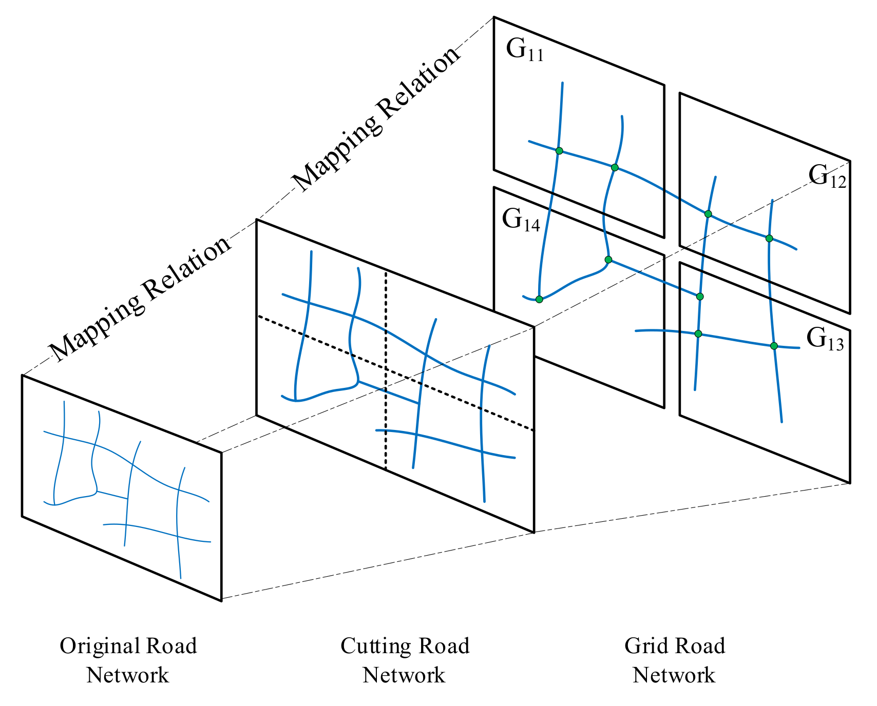
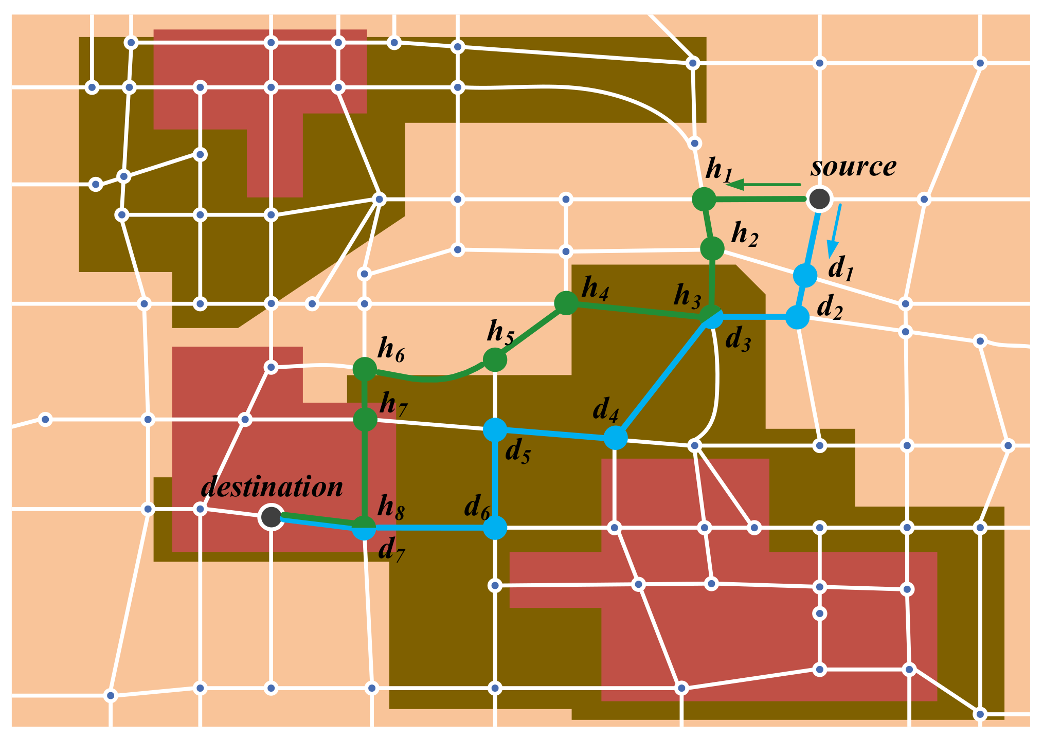
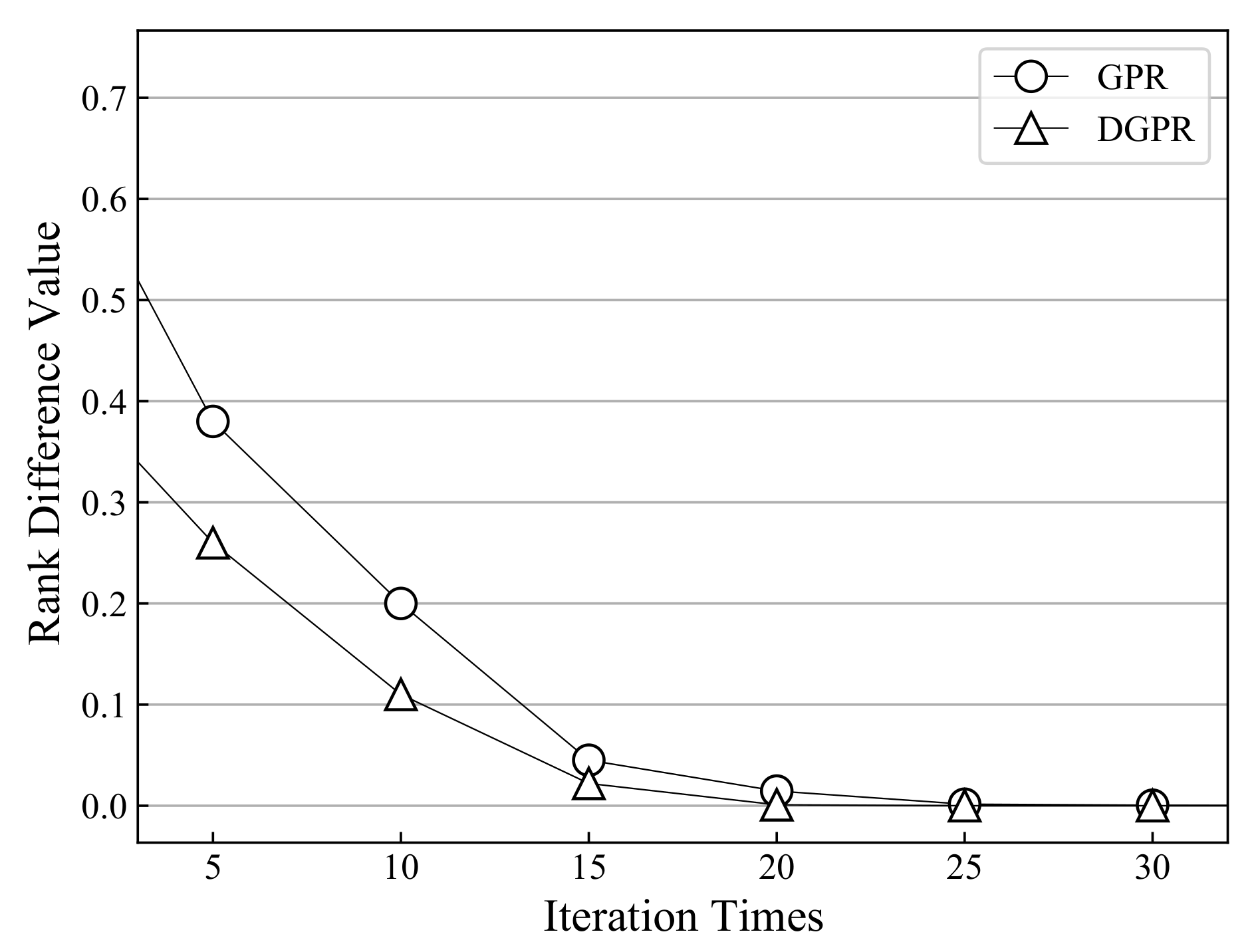
Table 1.
Notations.
| Notation | Definition |
|---|---|
| V | A set of intersection |
| A set of ordered pairs of vertices | |
| T | Represents the average time of the vehicle passing through the road of two intersections |
| The query time is taken into consideration | |
| Represents the average time of the vehicle passing through the road of two intersections | |
| Stands for the length of the road | |
| S | The average speed of the vehicle |
| Represents the number of partitions | |
| The whole city map in situational gird | |
| The grid map divides the entire map into several sub-maps | |
| Indicates a ratio of the number of intersections in the grid to the number of intersections in other grids | |
| The initial rank value of the ith grid | |
| The road weight with inbound the | |
| Stands a total number of vertices in ith grid | |
| N | The number of grid, all of which contain at least one intersection |
| Stands for the road network speed | |
| A rank matrix of real-time dynamic changes | |
| Represents a quaternion function of the ith grid | |
| Stands a activation function | |
| Represents the minimal step size between grids | |
| Represents the angle between two lines | |
| The result of grid DGPR | |
| Stands for road network maximum capacity factor | |
| The actual road network capacity factor |
Table 2.
List of Abbreviations.
| Abbreviation | Full Name |
|---|---|
| Evacuation Route Planning | |
| immune-based comprehensive Evacuation Planning | |
| Hybrid Spatio-temporal Graph Convolutional Network | |
| Dynamic Switch-Attention Network | |
| Multi-Space Attention | |
| Grid Map Emergency Path Planning | |
| Equidistant Grid Emergency Path Planning | |
| Situational Grid Road Network | |
| Grid Bidirectional Dijkstra | |
| Situational Grid Heuristic Search | |
| Contraction Hierarchies | |
| Situational Contraction Hierarchies | |
| Situational Grid Contraction Hierarchies | |
| Situational Grid Multiple Reverse Contraction Hierarchies | |
| Breadth-First Search | |
| Real-Time A* | |
| Linear Temporal Logic | |
| Linear Temporal Logic based A* | |
| Global Rover Horizontal Optimization Planner | |
| Rapidly-exploring Random Tree based A* | |
| Grid PageRank | |
| Dynamic Grid PageRank | |
| Hybrid Radial Function |
Table 3.
Comparison table of urban road network capacity.
| CRG | Unclassified | Tertiary | Secondary | Primary | Motorway |
|---|---|---|---|---|---|
| SL (km/h) | 30 | 4050 | 6070 | 80 | 90,120 |
| TC | 600 | 900 | 1060 | 1600 | 1800 |
| 0.10 | 0.15 | 0.18 | 0.27 | 0.30 |
Table 4.
The actual road network capacity mapping table.
| RS (km/h) | [0, 20) | [20, 30) | [30, 40) | [40, 60) | [60, 70) | [70, 80) | [80, 120) |
|---|---|---|---|---|---|---|---|
| TC | 150 | 600 | 900 | 1060 | 1330 | 1600 | 1800 |
| 0.02 | 0.09 | 0.12 | 0.14 | 0.17 | 0.22 | 0.24 |
Table 5.
Comparison with different query time window.
| SEVP | SGHS* | RV (avg) | RT (avg) | IT (avg) |
|---|---|---|---|---|
| 500 | = 2 (min) | 31,826 | 82.3 ms | 136 |
| = 5 (min) | 30,342 | 79.2 ms | 59 | |
| = 15 (min) | 34,721 | 85.8 ms | 27 | |
| = 30 (min) | 68,924 | 182.1 ms | 23 | |
| = 45 (min) | 101,936 | 242.4 ms | 11 | |
| = 60 (min) | 328,611 | 432.3 ms | 5 | |
| 1000 | = 2 (min) | 30,582 | 83.6 ms | 129 |
| = 5 (min) | 33,617 | 85.5 ms | 60 | |
| = 15 (min) | 36,436 | 84.7 ms | 25 | |
| = 30 (min) | 71,322 | 174.2 ms | 18 | |
| = 45 (min) | 131,936 | 302.3 ms | 9 | |
| = 60 (min) | 325,349 | 452.6 ms | 4 | |
| 2000 | = 2 (min) | 32,481 | 78.9 ms | 144 |
| = 5 (min) | 31,342 | 77.2 ms | 69 | |
| = 15 (min) | 36,552 | 81.7 ms | 21 | |
| = 30 (min) | 68,980 | 179.1 ms | 20 | |
| = 45 (min) | 126,450 | 212.4 ms | 12 | |
| = 60 (min) | 333,414 | 458.1 ms | 6 | |
| 3000 | = 2 (min) | 34,255 | 79.5 ms | 125 |
| = 5 (min) | 37,279 | 79.7 ms | 67 | |
| = 15 (min) | 35,727 | 83.2 ms | 24 | |
| = 30 (min) | 69,902 | 187.9 ms | 18 | |
| = 45 (min) | 123,592 | 202.4 ms | 10 | |
| = 60 (min) | 321,895 | 428.5 ms | 5 |
Table 6.
Different of Effect Based Different Distributions with Four Paths.
| Methods | P1 = 5.3 km | p2 = 17.5 km | p3 = 30.4 km | p4 = 49.8 km | ||||||||
|---|---|---|---|---|---|---|---|---|---|---|---|---|
| Dijkstra | ∗ | 98 | 23.3 | ∗ | 892 | 78.9 | ∗ | 5432 | 226.2 | ∗ | 19311 | 404.9 |
| A* | ∗ | 79 | 22.6 | ∗ | 781 | 68.8 | ∗ | 3572 | 189.7 | ∗ | 12477 | 362.7 |
| T* | ∗ | 71 | 21.4 | ∗ | 708 | 69.3 | ∗ | 3523 | 183.4 | ∗ | 11584 | 358.4 |
| RTA* | ∗ | 75 | 20.5 | ∗ | 774 | 73.1 | ∗ | 3629 | 165.8 | ∗ | 12831 | 346.3 |
| RRT* | ∗ | 84 | 19.8 | ∗ | 817 | 72.4 | ∗ | 3641 | 172.1 | ∗ | 11425 | 334.1 |
| GBD | 15 | 35 | 18.2 | 78 | 343 | 69.8 | 213 | 1710 | 179.9 | 354 | 3482 | 347.5 |
| SGHS* | 15 | 39 | 21.4 | 63 | 338 | 68.5 | 175 | 1696 | 173.5 | 247 | 3369 | 340.9 |
Table 7.
Comparison the results of vehicle travel time with clear and congestion in different path distances.
Table 7.
Comparison the results of vehicle travel time with clear and congestion in different path distances.
| Case | Methods | P1 (5.3 km) | P2 (17.5km) | P3 (30.4km) | P4 (49.8 km) |
|---|---|---|---|---|---|
| non-congestion | Dijkstra | 15.4 (min) | 30.2 (min) | 49.4 (min) | 65.5 (min) |
| A* | 16.5 (min) | 28.9 (min) | 48.5 (min) | 66.8 (min) | |
| T* | 15.1 (min) | 28.8 (min) | 49.6 (min) | 64.6 (min) | |
| RTA* | 15.7 (min) | 26.6 (min) | 44.1 (min) | 66.3 (min) | |
| RRT* | 15.4 (min) | 27.3 (min) | 42.7 (min) | 64.8 (min) | |
| GBD | 16.3 (min) | 25.5 (min) | 43.9 (min) | 65.5 (min) | |
| SGHS* | 16.0 (min) | 27.4 (min) | 44.3 (min) | 66.3 (min) | |
| congestion | Dijkstra | 17.2 (min) | 42.6 (min) | 94.3 (min) | 133.8 (min) |
| A* | 17.7 (min) | 38.5 (min) | 88.7 (min) | 122.9 (min) | |
| T* | 16.9 (min) | 35.9 (min) | 81.2 (min) | 113.5 (min) | |
| RTA* | 17.8 (min) | 37.1 (min) | 83.4 (min) | 124.1 (min) | |
| RRT* | 17.5 (min) | 39.4 (min) | 85.7 (min) | 127.2 (min) | |
| GBD | 16.1 (min) | 32.3 (min) | 79.4 (min) | 108.4 (min) | |
| SGHS* | 16.3 (min) | 30.7 (min) | 71.8 (min) | 98.7 (min) |
Table 8.
Comparison with different graph contraction methods.
| Methods | Vertex | Edge | Grid | CV | CG | Shortcut | RT (ms) |
|---|---|---|---|---|---|---|---|
| CH | 500 | 1548 | 70 | 76 | ∗ | 52 | 5 |
| 1000 | 3603 | 140 | 159 | ∗ | 104 | 9 | |
| 3000 | 9864 | 560 | 406 | ∗ | 321 | 59 | |
| 5000 | 16,926 | 700 | 887 | ∗ | 538 | 120 | |
| 10,000 | 32,510 | 1400 | 2193 | ∗ | 1384 | 692 | |
| 20,000 | 63,721 | 2800 | 4579 | ∗ | 3492 | 1501 | |
| 83,884 | 222,778 | 82,944 | 19,395 | * | 15,596 | 16,613 | |
| SCH | 500 | 1548 | 70 | 24 | ∗ | 19 | 6 |
| 1000 | 3603 | 140 | 95 | ∗ | 68 | 11 | |
| 3000 | 9864 | 560 | 169 | ∗ | 129 | 62 | |
| 5000 | 16,926 | 700 | 421 | ∗ | 335 | 168 | |
| 10,000 | 32,510 | 1400 | 1593 | ∗ | 1202 | 772 | |
| 20,000 | 63,721 | 2800 | 3979 | ∗ | 2874 | 1883 | |
| 83,884 | 222,778 | 82,944 | 12,599 | * | 9596 | 16,542 | |
| SGCH | 500 | 1548 | 70 | 95 | 8 | 79 | 9 |
| 1000 | 3603 | 140 | 209 | 29 | 175 | 18 | |
| 3000 | 9864 | 560 | 1092 | 81 | 321 | 139 | |
| 5000 | 16,926 | 700 | 1907 | 172 | 1274 | 308 | |
| 10,000 | 32,510 | 1400 | 3080 | 271 | 1983 | 992 | |
| 20,000 | 63,721 | 2800 | 5227 | 425 | 3062 | 2191 | |
| 83,884 | 222,778 | 82,944 | 25,612 | 1291 | 18,233 | 18,238 | |
| SGMRCH | 500 | 1548 | 70 | 107 | 8 | 82 | 11 |
| 1000 | 3603 | 140 | 359 | 32 | 186 | 29 | |
| 3000 | 9864 | 560 | 606 | 89 | 363 | 193 | |
| 5000 | 16,926 | 700 | 2589 | 186 | 1370 | 531 | |
| 10,000 | 32,510 | 1400 | 4185 | 281 | 1989 | 1592 | |
| 20,000 | 63,721 | 2800 | 7579 | 432 | 3296 | 3659 | |
| 83,884 | 222,778 | 82,944 | 29,341 | 1284 | 18,935 | 19,032 |
Publisher’s Note: MDPI stays neutral with regard to jurisdictional claims in published maps and institutional affiliations. |
© 2021 by the authors. Licensee MDPI, Basel, Switzerland. This article is an open access article distributed under the terms and conditions of the Creative Commons Attribution (CC BY) license (https://creativecommons.org/licenses/by/4.0/).
Share and Cite
MDPI and ACS Style
Yang, B.; Yan, J.; Cai, Z.; Ding, Z.; Li, D.; Cao, Y.; Guo, L. A Novel Heuristic Emergency Path Planning Method Based on Vector Grid Map. ISPRS Int. J. Geo-Inf. 2021, 10, 370. https://doi.org/10.3390/ijgi10060370
AMA Style
Yang B, Yan J, Cai Z, Ding Z, Li D, Cao Y, Guo L. A Novel Heuristic Emergency Path Planning Method Based on Vector Grid Map. ISPRS International Journal of Geo-Information. 2021; 10(6):370. https://doi.org/10.3390/ijgi10060370
Chicago/Turabian StyleYang, Bowen, Jin Yan, Zhi Cai, Zhiming Ding, Dongze Li, Yang Cao, and Limin Guo. 2021. "A Novel Heuristic Emergency Path Planning Method Based on Vector Grid Map" ISPRS International Journal of Geo-Information 10, no. 6: 370. https://doi.org/10.3390/ijgi10060370
Note that from the first issue of 2016, this journal uses article numbers instead of page numbers. See further details here.