Article

A Spatial Multi-Criteria Model for the Evaluation of Land Redistribution Plans

1
School of Geography, University of Leeds, Leeds LS2 9JT, UK
2
International Institute of Applied Systems Analysis (IIASA), Schlossplatz 1, A-2361 Laxenburg, Austria
3
Centre for Advanced Spatial Analysis (CASA), University College London (UCL), London WC1E 6BT, UK
*
Author to whom correspondence should be addressed.
ISPRS Int. J. Geo-Inf. 2012, 1(3), 272-293; https://doi.org/10.3390/ijgi1030272
Submission received: 18 August 2012 / Revised: 23 October 2012 / Accepted: 26 October 2012 / Published: 9 November 2012

Abstract

:
A planning support system for land consolidation has been developed that has, at its heart, an expert system called LandSpaCES (Land Spatial Consolidation Expert System) which contains a “design module” that generates alternative land redistributions under different scenarios and an “evaluation module” which integrates GIS with multi-criteria decision making for assessing these alternatives. This paper introduces the structural framework of the latter module which has been applied using a case study in Cyprus. Two new indices are introduced: the “parcel concentration coefficient” for measuring the dispersion of parcels; and the “landowner satisfaction rate” for predicting the acceptance of the land redistribution plan by the landowners in terms of the location of their new parcels. These two indices are used as criteria for the evaluation of the land redistribution alternatives and are transferable to any land consolidation project. Moreover, a modified version of the ratio estimation procedure, referred to as the “qualitative rating method” for assigning weights to the evaluation criteria, is presented, along with a set of non-linear value functions for standardizing the performance scores of the alternatives and incorporating expert knowledge for five evaluation criteria. The application of the module showed that it is a powerful new tool for the evaluation of alternative land redistribution plans that could be implemented in other countries after appropriate adjustments. A broader contribution has also been made to spatial planning processes, which might follow the methodology and innovations presented in this paper.

1. Introduction

Land fragmentation occurs when single landholdings consist of numerous spatially separated land parcels [1]. Land consolidation is considered to be the most effective land management approach for solving this problem and is undertaken in many countries around the world [2,3]. Land consolidation includes the process of land reallocation, which can itself be divided into two sub-processes, land redistribution and land partitioning. Land redistribution comprises the preparation of a preliminary plan to restructure land parcels in terms of their number, ownership, size, value and approximate location based on legislation, the existing land tenure structure, rules of thumb and the experience of the planner. For example, in Cyprus, the development of such a plan requires that a team of land consolidation planners meet with each land owner in order to understand their preferences, the most important aspect being where their new parcels should be located. An acceptable plan, determined from a set of alternatives is then drawn up, which forms the basis of land partitioning in which new parcels are created that consolidate the land holdings and minimize the amount of spatial separation between the parcels belonging to each landowner.
One problem with the land consolidation process is the amount of time needed to complete each land consolidation project. For example, the average project duration is 8–16 years in Germany, 10–12 years in the Netherlands, 8–12 years in Finland and 5–7 years in Sweden [4]. In Cyprus, a project takes on average from 6 to 10 years [5] with 2–3 years spent on the preparation of the land reallocation plan. The amount of time required is partly a function of the lack of adequate tools to support land consolidation, since proprietary geographic information systems (GIS) are not capable of handling the complexity involved. Demetriou et al. [6] have proposed a framework for an integrated planning and decision support system (IPDSS) which encapsulates the entire land reallocation process into an automated workflow. Using this framework embedded within a GIS environment, the LAnd CONsolidation Integrated Support System for planning and decision making (LACONISS) system was developed, which consists of three main sub-systems: a Land Fragmentation System (LandFragmentS) [7]; a Land Spatial Consolidation Expert System (LandSpaCES) [8]; and a Land Parcelling System (LandParcelS) [9].
This paper is specifically concerned with a methodology for evaluation but we must acknowledge that evaluation in the context of land consolidation may have different meanings according to whether it refers to suitability evaluation, comprehensive project evaluation or land reallocation plan evaluation. Suitability evaluation studies [10,11,12] are carried out before project implementation and aim to investigate the potential for applying land consolidation. Comprehensive evaluation studies [13,14,15,16,17,18] are broad based and consider the potential impacts of the whole project usually in terms of three main components: economic efficiency which is related to the improvement of land fragmentation indices and the consequent agricultural benefits (e.g., production, productivity, farmers’ income); environmental impacts; and social impacts covering the potential project impacts to landowners or a group of people or to society as a whole. This kind of evaluation can be applied ex-ante or ex-post with the latter being the most usual case. The third type of evaluation, i.e., land reallocation plan evaluation studies [19,20,21,22] has a narrow scope, focusing on the quality of the land reallocation plan during the design stage, i.e., ex-ante evaluation. However, existing studies do not present any methodological developments in this area because they use isolated indices regarding land fragmentation such as the size, shape and dispersion of parcels and hence they do not provide a systematic method for evaluating land reallocation or land redistribution plans. One reason may be that land reallocation plans are usually generated manually, resulting in a single (although not necessarily optimal) solution.
Thus, within the LACONISS system, the LandSpaCES sub-system consists of two components. The first is a “design module”, which is an expert system (ES) that can generate alternative land redistribution solutions [8] in an automated way. The second is an “evaluation module” that integrates GIS with a multi-attribute decision-making method (MADM) to evaluate these solutions efficiently and systematically according to the specific needs of each land consolidation project and to assist in the selection of an optimum solution. The purpose of this paper is to outline the methodology that we have developed for this evaluation process, which is embedded within LandSpaCES and which incorporates new concepts such as the “parcel concentration coefficient” (PCC) for characterizing parcel dispersion and the “landowner satisfaction rate” (LSR) which attempts to capture the preferences of each landowner in an automated way. The methodology is then demonstrated on a real land consolidation case study in Cyprus where ten alternative land redistribution solutions have been generated under a set of different scenarios. More details of the generation of these alternative land redistribution solutions can be found in Demetriou et al. [8].

2. Methodology

The evaluation of alternative land redistribution plans uses multi-attribute decision making (MADM) methods [23,24] which attempt to find the best solution among a discrete number of alternative solutions. The process is illustrated in Figure 1 where initially a set of alternative land redistributions is generated and the planner has to select a set of evaluation criteria to assess these alternatives. This produces an effect table with the alternatives in columns and the criteria in rows. The performance of each alternative for each criterion is represented by a score that constitutes an element of the effect table located in a cell of the matrix. The scores are standardized to values between 0 and 1 (representing worst and best performances of alternatives, respectively) and weights are chosen for each criterion by the planner. The decision rules comprise the evaluation method utilized in order to rank the alternatives. Finally, a sensitivity analysis is carried out aimed at assessing the robustness of the ranking order followed by the output of a final recommendation about the most beneficial solution. Each component of the process is now explained in further detail in the sections that follow. The entire process described above has been embedded in a GIS environment (i.e., ArcGIS) by utilizing VBA and ArcObjects [25,26]. Several authors refer to the integration of multi-criteria methods with GIS [27,28,29,30]. The role of GIS is critical in both designing and evaluating the alternative solutions [8]. In terms of the latter, GIS automatically provides all the metrics of each alternative for each of the evaluation criteria involved, a task that would be impossible to carry out manually or through using conventional non-spatial systems since the spatial component of the problem significantly increases the complexity of the calculations.
Figure 1. General model of multi-attribute decision-making method (MADM) (adapted from Sharifi et al. [31]).
Ijgi 01 00272 g001

2.1. Evaluation Criteria

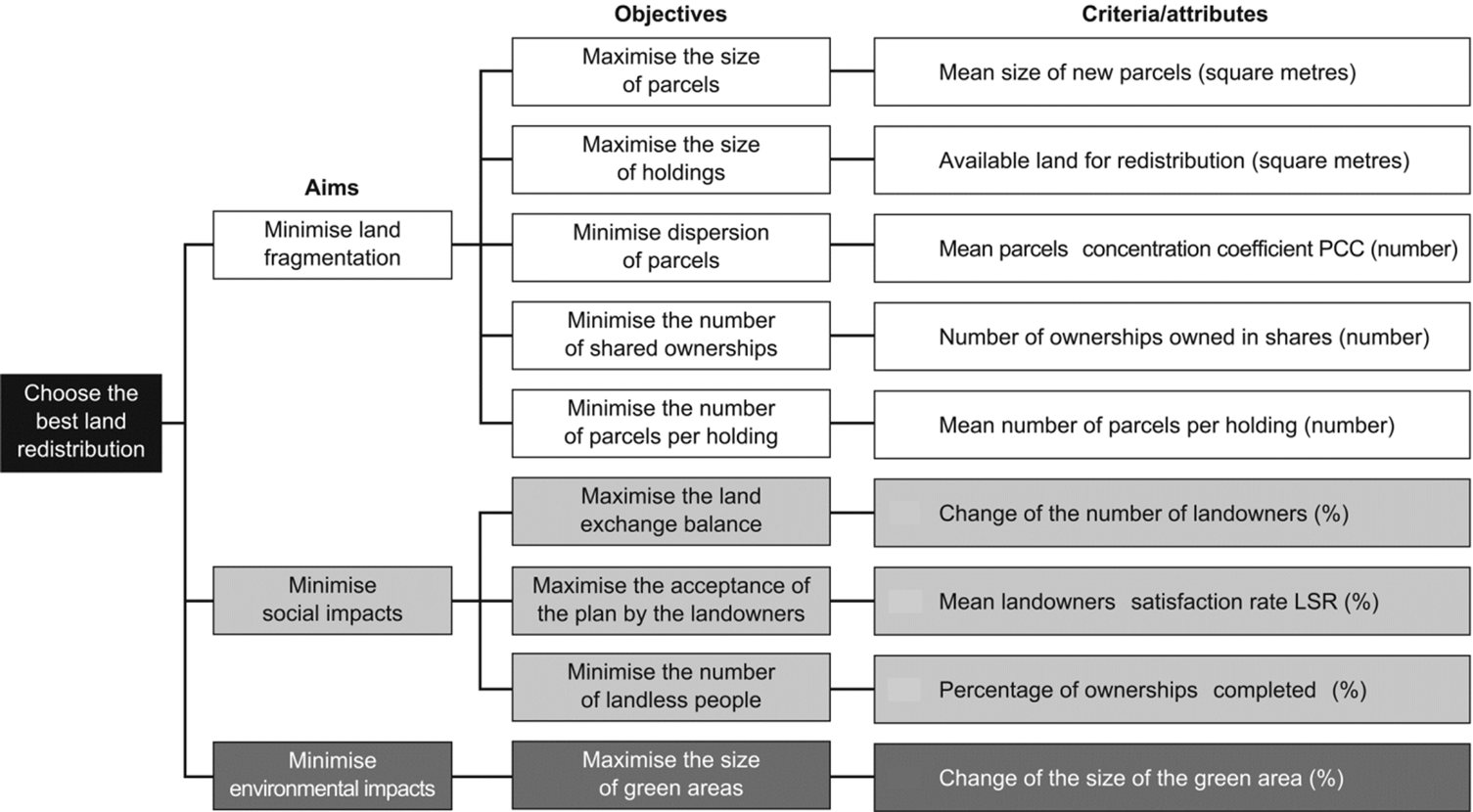
The selection of the appropriate criteria begins with the definition of a hierarchical objective tree specified via the goal, aims and objectives of the land consolidation problem [32]. Thereafter, a specific land redistribution objective tree can be formulated (Figure 2) which contains the aims, objectives and the corresponding criteria/attributes, which can be used in the evaluation of the alternative land redistribution plans.
Whilst 
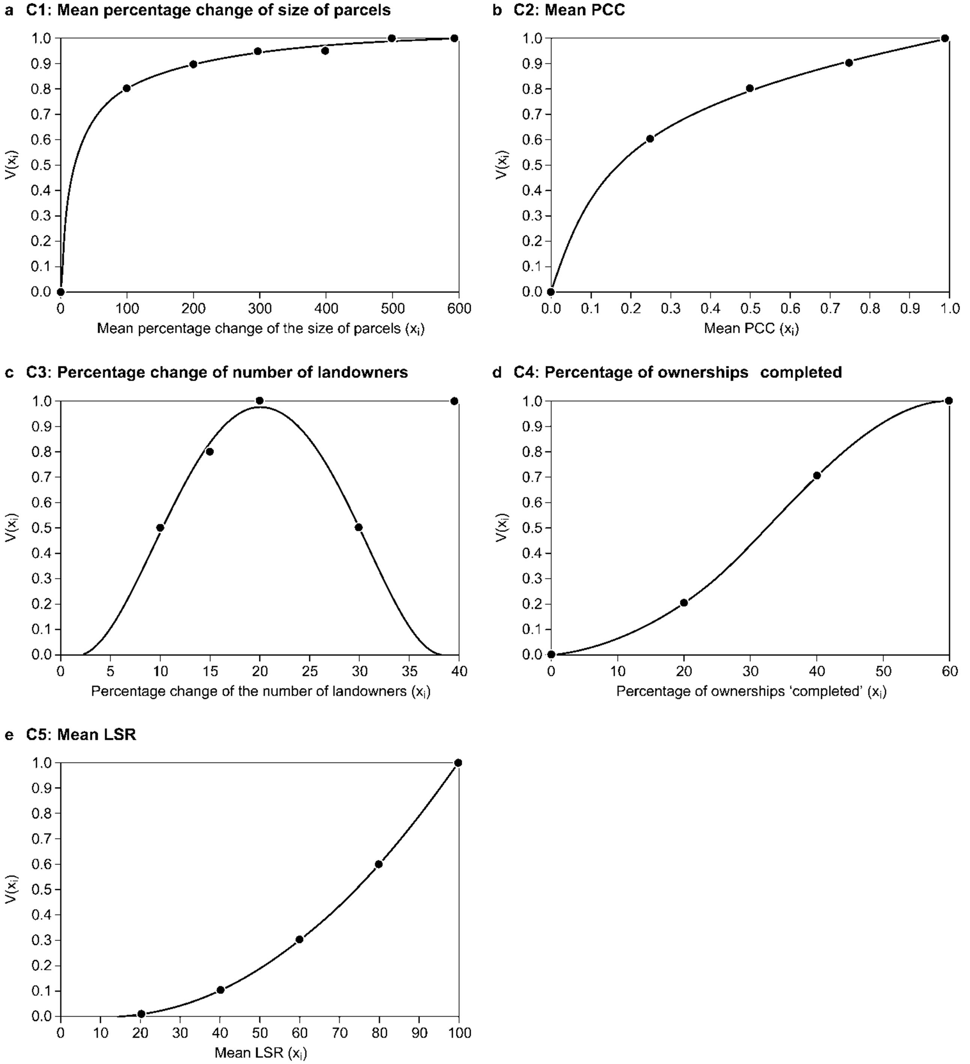
Figure 2 shows nine possible criteria, Demetriou et al. [32] suggest that only the following five criteria are required: the mean size (as a percentage change before and after applying a solution) of the new parcels (C1); the mean parcel concentration coefficient (C2); the change (as a percentage) in the number of landowners (C3); the percentage of ownerships “completed” involving the percentage of ownerships that had less than the minimum size limit provided by legislation and “complete” to reach that minimum limit (C4); and the mean landowner satisfaction rate (C5). Both the PCC and LSR are new concepts, which are explained in more detail below.
Figure 2. The objective tree for the land redistribution problem.
Ijgi 01 00272 g002

2.1.1. Parcel Concentration Coefficient (PCC)

A basic measure of spatial dispersion is standard distance which is the spatial equivalent of the standard deviation, showing how locations or points are scattered around the spatial mean [33,34]. The spatial mean or mean center of gravity is an important spatial statistical measure of central tendency which indicates the average location of a set of points defined in a Cartesian coordinate system. Thus, standard distance measures the degree to which parcels (or more precisely the centroids of parcels) are concentrated or dispersed around their geometric mean. Although, in practice, the dispersion of holdings is dependent on the location of the farmstead or the village where the farmer resides, and in this case transport distances could be calculated based on some assumptions [21], the extra information needed is usually not available, so the mean center of parcels of a holding is a proxy criterion that gives an adequate representation of the dispersion before and after land consolidation.
An extension of both statistics is the weighted mean center and the weighted standard distance where centroids may have different attribute values representing the different sizes or land values of each parcel. For instance, if the largest parcels of a holding are very much dispersed in terms of location, this may have greater negative effects on production, productivity, labor and hence the income of farmer, than if the smaller parcels are dispersed [19]. Thus, the weighted mean center of a holding is a better indicator than the simple mean center because it reflects not only the spatial dispersion of parcels but also the agricultural importance of each parcel.
Expressing these spatial statistics in the context of land consolidation, the mean center of the parcels of a holding can be expressed as:
Ijgi 01 00272 i003
where xhmc and yhmc are the co-ordinates of the mean center of the holding; xi and yi are the co-ordinates of the centroid of parcel i; and n is the number of parcels belonging to a holding. The weighted mean center of a holding can be calculated in a similar way as:
Ijgi 01 00272 i004
where xwhmc and ywhmc are the co-ordinates of the weighted mean center of the holding and wi is the weight of each parcel i. From these quantities, the dispersion of parcels (DoP) and the weighted version of DoP can be calculated as:
Ijgi 01 00272 i005
Ijgi 01 00272 i006
where both measures have been utilized previously by Tourino et al. [19]. However, the disadvantage of these measures is that they may vary across an unlimited range of values with no explicit extreme values, which renders interpretation difficult. In this research, a new indicator is developed called the parcel concentration coefficient (PCC) for each holding which is measured on a scale between −1 and 1. A value of zero indicates no change in the dispersion of a holding’s parcels before and after land consolidation. The value of +1 refers to the situation of “perfect concentration” while −1 represents the “worst concentration”. The DoP can be calculated for each holding twice, i.e., before (DoPb) and after (DoPa) land consolidation and then combined to calculate the PCC for three situations:
  • If DoPb = DoPa then PCC = 0 and the dispersion of parcels has not changed.
    In this situation, land consolidation has not achieved any concentration of parcels for the holding concerned independently of the number of new parcels allocated to a landowner (n') or the number of original parcels owned by the landowner (n).
  • If DoPb > DoPa the PCC can be expressed as:
    Ijgi 01 00272 i007
    In this situation, an improvement in the dispersion of parcels has occurred. The maximum value of 1 means that parcels have been concentrated after land consolidation into a single parcel, i.e., n' = 1 and perfect concentration has been achieved. This happens when the DoPa equals 0 and consequently n' = 1. The numerator in Equation (5) represents the proportional change of dispersion before and after land consolidation of a holding. The denominator, i.e., n', adjusts the proportional change in dispersion (the level of concentration) since the PCC increases as n' decreases. In other words, the higher n', the less the concentration of new parcels and hence PCC reduces towards a value of zero.
  • If DoPb < DoPa, then the PCC is expressed as:
    Ijgi 01 00272 i008
In this situation, deterioration in the dispersion of parcels has occurred. This may occur when either n' is greater than n (which is a very rare case) and/or when the parcels have been allocated at greater distances. The extreme value of −1 means that the concentration of parcels after land consolidation has worsened independent of the number of new parcels allocated since the basic aim of concentrating parcels via land consolidation has completely failed. This happens when the DoPb equals 0 and consequently n = 1. The denominator n adjusts the proportional change in dispersion, i.e., the level of concentration, since the PCC increases as n increases. In other words, the greater the value of n, the less extreme the difference (before and after a project) in parcel concentration and hence PCC reduces towards zero because the dispersion was already poor.

2.1.2. Landowner Satisfaction Rate (LSR)

The landowner satisfaction rate (LSR) is an indicator that captures the satisfaction of the landowners with regard to their preferences in terms of the location of their new parcels. It is based on the parcel priority index (PPI) introduced in Demetriou et al. [8], which ranks the preferences of the landowners regarding the locations of the new parcels they wish to receive. The calculation of the LSR involves determining which preferences of each landowner have been satisfied and assigns a proportional percentage of satisfaction (called the partial satisfaction rate, PSR) to each new parcel depending on the ranking of the preference satisfied, with a maximum of 100%. A critical point in this process is that the original parcels of a landowner (n), which are already in preference ranking order, are divided into two parts. The first covers the situation up to n' whilst the other part covers the situation for the rest of the parcels, i.e., from nn'. Thus, if a new parcel falls in the first part, the PSR will be 100% but if it falls in the second part, then the PSR is assigned proportionally, i.e., reduced, depending on n and n′. This can be expressed mathematically as follows:
If n n' then the PSR for each new parcel i allocated to a landowner can be calculated as follows:
Ijgi 01 00272 i009
where mi is a variable that takes into account the number of parcels originally owned by a landowner (n) and the rank order of the preference of each original parcel i (ROi), and P is a linear function that expresses decreasing satisfaction for each landowner. The two variables, mi and P are computed as follows:
Ijgi 01 00272 i010
Maxmi is the mi value assigned to those new parcels that fall in the first part of original parcels as explained earlier. In this case, the parameter ROi in Equation (8) is replaced by the number of new parcels (n') as follows:
Ijgi 01 00272 i011
P is a constant percentage for the redistribution of each holding which is calculated based on the two parts mentioned earlier. In particular, the parcels that belong in the first part count as one sub-part whilst the parcels that belong in the second part count as a separate sub-part. Thus, P results by dividing 100% by the total number of sub-parts which always equals n−n'+1. Therefore, P can be computed as:
Ijgi 01 00272 i012
Combining Equations (8) and (10) yields:
Ijgi 01 00272 i013
The total LSR for each landowner j is then calculated as the mean value of the PSR:
Ijgi 01 00272 i014
Similarly, the average LSR for the whole land consolidation area, i.e., the whole project, can be calculated as the mean LSR of all landowners (l) who received property in the plan as follows:
Ijgi 01 00272 i015
The above assumptions become clearer by utilizing an example for calculating PSR and LSR. An example is provided in Table 1 which involves a landowner who originally had five parcels (i.e., n = 5) and after land consolidation receives 1, 2 or 3 parcels (i.e., n' = 1 to 3). Each cell of the table contains the PSR value for each combination of n and n'.
Table 1. An example for the calculation of the partial satisfaction rate.
Number of New Parcels (n') Allocated to the Landowner
n123
1maxM × P = 5× 20 = 100%maxM × P = 4× 25 = 100%maxM × P = 3× 33.33 = 100%
2M2 × P =(5 – 2 + 1)× 20 = 80%maxM × P = 4× 25 = 100%maxM × P = 3× 33.33 = 100%
3M3 × P = (5 – 3 + 1)× 20 = 60%M3 × P = (5 – 3 +1 )× 25 = 75%maxM × P = 3× 33.33 = 100%
4M4 × P = (5 – 4 + 1)× 20 = 40%M4 × P = (5 – 4 + 1)× 25 = 50%M4 × P = (5 – 4 + 1)× 33.33 = 66.66%
5M5 × P = (5 – 5 + 1)× 20 = 20%M5 × P = (5 − 5 + 1)× 25 = 25%M5 × P = (5 – 5 + 1)× 33.33 = 33.33%
For example, if a landowner has been allocated one parcel (i.e., first column) in the same location as its fourth preference (i.e., fourth row), then the PSR and hence the LSR (because n' = 1) is 40%. Similarly, if the landowner has been allocated two parcels (i.e., second column), say in the same location as the first (i.e., first row) and fourth preference (i.e., fourth row), then the PSR is 100% and 50% for the location of the first parcel and second parcel, respectively. In this case, the average LSR is calculated as 75%.

2.2. Weighting the Criteria

There are several methods available to weight the evaluation criteria including direct ranking; swing weights; ranking; rating; pairwise comparison; trade off analysis; and qualitative translation [23,31,35]. The most popular are the ranking and rating methods because of their simplicity. However, there are problems with assigning weights to a fine scale, e.g., to two decimal points in the direct ranking method. In addition, other ranking methods (e.g., the rank sum, rank reciprocal and rank exponent method) do not provide the potential to rank two or more criteria with equal importance, which is relevant for this problem. To develop a simple fit-for-purpose method that allows planners to assign weights while overcoming the aforementioned problems, a modified version of the ratio estimation procedure has been developed that uses a similar qualitative scale as found in pair-wise comparison method is hereafter called the “qualitative rating method”. The criteria are classified into the following seven classes of importance: extremely high; very high; high; intermediate; moderate; low; and very low, which are more intuitive to rank than a number or score, and the criteria may have the same importance using this method. Each class has a predefined range of importance from 0 to 100 as shown in Table 2 but the rate of increase in importance in the lower part of the scale is 10 points whilst in the upper part it is double, i.e., 20 points. This represents an imposed weighting in favor of the higher classes. Although this scoring seems arbitrary, in practice this is realistic since planners and decision makers tend to ignore the less important criteria in the decision-making process. After selecting the importance of each criterion, the weights are standardized based on the score assigned to each criterion so that the weights sum to 1.
Table 2. The scale of importance and the relevant scores utilized by the qualitative rating method.
Rank OrderScale of ImportanceScoreClasses
1Extremely high100Upper
2Very high80
3High60
4Intermediate40Middle
5Moderate30Lower
6Low20
7Very low10
Whatever method is employed for assigning weights to criteria, the planner needs to be aware that the weights of the criteria should be aligned with the range of the corresponding performance scores [35,36]. In other words, the larger the range of a performance score for a criterion, the greater the importance (hence the weight) of that criterion in terms of its contribution in the ranking of alternatives. This is known as the range sensitivity principle [37].

2.3. Standardization Process

Standardization (or normalization) is the process of transforming the scores of the evaluation criteria into the same scale so that they can be combined and compared. Several standardization methods have been developed, which generally fall into: linear scale transformations [23,31] and value/utility function approaches. Linear methods (maximum, interval and goal standardization) are most commonly adopted because of simplicity and a predefined behavior but they have two main disadvantages. First, they assume a linear association between the original values and the standardized values when, in practice, this relationship is more complex; and second, they ignore the judgments of the decision makers as they have no input in the development of the simple linear standardization functions that are commonly used. These limitations are overcome by using value functions, which encapsulate human judgment in a mathematical form. These functions translate the performance score of an alternative for a criterion into a value score between 0 and 1, representing the degree to which a certain decision objective is achieved. A number of methods have been developed for the creation of value functions. The most common are the midvalue, Evalue and direct rating methods [35]. The latter has been utilized in this research because of simplicity and flexibility in terms of assigning values that depend on the criterion concerned. Direct value rating involves the following five steps for each criterion:
  • Identify the minimum and maximum values of the criterion which correspond to values of 0 (worst) and 1 (best), respectively. In the context of this research, the minimum and maximum values for criteria C1, C3 and C4 were identified from 40 year statistical records provided by the Land Consolidation Department (LCD) of Cyprus for 74 land consolidation projects. For criteria C2 and C5, the minimum values are zero and the maximum values are 1 and 100%, respectively.
  • Define characteristics of the value function, i.e., monotonicity, shape, etc.
  • Assign values to selected criterion scores at equal intervals between the minimum and maximum.
  • Fit a mathematical equation through these points using appropriate software.
  • Validate the functions as representations of preference.
The values functions for C1 to C5 for the Cyprus case study are presented in Figure 3(a–e) and as Equations (14–18) respectively.
Figure 3(a) shows a concave benefit value function for the mean percentage change in the size of parcels represented as:
Ijgi 01 00272 i016
The value function increases sharply from 0 to 0.8 since the latter value corresponds to 100%, a score considered by experts as easily achievable, and then gradually increases up to the maximum score of 600% which is the highest ever achieved in land consolidation projects. Figure 3(b) is another concave benefit value function for mean PCC:
Ijgi 01 00272 i017
A maximum score of 1 which denotes perfect concentration of parcels whilst a minimum of 0 means that nothing has changed in terms of the parcel concentration after land consolidation. A mean PCC of more than 0.5 (which corresponds to a value of 0.8 or 80%) is highly satisfactory for the experts, since on most occasions, it is not always possible to join all the parcels of a holding into a single parcel.
Figure 3. The value functions for the evaluation criteria.
Ijgi 01 00272 g003
Figure 3(c) shows a mixed bell-shaped benefit-cost value function for the percentage change in the number of landowners:
Ijgi 01 00272 i019
The curve increases rapidly from 0 to the peak (20%) where this range includes holdings that are much smaller in size than the minimum limits provided by legislation. These properties will be redistributed (by compensation) to the other landowners either mainly to “complete” their property at the minimum size or increase the size of other properties. The rest of the function then falls steeply from 20% to 40%, which represents a negative effect since a high percentage of landless landowners would be generated, with many not agreeing to leave their property for compensation.
Figure 3(d) shows an s-shaped benefit value function for percentage of ownerships completed:
Ijgi 01 00272 i020
The convexity in the first part of the function (0 to 25%) represents a low satisfaction rate for the objective. The second linear section (25 to 40%) presents a significant increase in satisfaction where many land redistribution alternatives are expected to fall. The final concave section (40 to 60%) is the most desirable in terms of alternative performance but is the most difficult to achieve. The final benefit value function represents the mean LSR as a convex curve (Figure 3(e)):
Ijgi 01 00272 i021
This function increases slowly from 0 to 60% corresponding to values of 0 to 0.3, respectively, representing low importance and then increases steeply between 60 to 90%, representing the most significant part of the function. Thus, the objective “to maximize the acceptance of the plan by the landowners” is achieved only at high values, i.e., greater than 80%.

2.4. Ranking the Alternatives

A value function approach is then utilized for ordering the alternative land redistributions, which is the weighted average of the single attribute values:
Ijgi 01 00272 i022
where Vj is the overall value (or performance score) of the jth alternative (j = 1 to M), vij is the standardized value of the score αij of the jth alternative with respect to the ith criterion/attribute (i = 1 to N) measured by utilizing an appropriate value function, and wi is the normalized weight for criterion/attribute i such that:
Ijgi 01 00272 i023
The alternative with the highest Vj is the best alternative compared with the other competitive alternative solutions.
It is noted that in contrast to the value function approach, other popular aggregation methods that can be utilized for evaluating a set of discrete alternatives include outranking methods that involve a pairwise comparison between all the alternatives. Chakhar and Mousseau [38] proposed a general framework to incorporate these methods into a GIS.

2.5. Sensitivity Analysis

Sensitivity analysis (SA) investigates the impact of changes in the inputs on the decision outcomes. It is a critical task for decision-making processes since it reveals how reliable the final decisions are [30]. For MADM, two important elements need to be examined: the weights of the evaluation criteria and the criterion scores (or performance measures) [23,39]. However, SA is not common practice in spatial multi-criteria decision problems, and where it has been used, only the sensitivity of the weights has been considered [40].The sensitivity of criterion weights is crucial because the process of assigning weights is subjective and may demonstrate significant variation between the decision makers’ perceptions and preferences. In addition, the available methods for defining the weights may lead to different results. Thus, a decision maker can take better decisions if he/she is aware of how critical each criterion is. Triantaphyllou [37,41] developed a methodology for individual decision making, which calculates the percentage change needed to alter the current weight of each relevant criterion so as to reverse the ranking order of the corresponding pair of alternatives for each combination of alternative pairs and for each criterion. The “percent top critical criterion” (that may alter the ranking of the best alternative), the “percent any critical criterion” (that may alter the ranking of any alternative) and a sensitivity coefficient for each criterion can be calculated. In the case of group decision making, e.g., in multi-stakeholder participatory processes, other methods can be used such as that provided by Jankowski et al. [42] in their web-based Choice Modeler system that involves extensive sensitivity analysis capabilities at three different levels (global, local and spatial).
In addition, the standardization process of utilizing value functions also involves considerable subjectivity, since the value functions have been defined by experts and the process of assessing them is inherently prone to uncertainties. The percentage change needed to alter the current performance score (of the first alternative from the pair) so as to reverse the rank order of the corresponding pair of alternatives for each combination of alternative pairs and for each criterion can be calculated [37,41].From this, the “most critical alternative”, the competing alternative to the best alternative, and the percentage change in the relevant performance score that will alter the ranking can be calculated. The above methodology has been incorporated into the evaluation module of LACONISS and is applied in the case study described in the next section.

3. Case Study

The evaluation methodology has been applied to an actual land consolidation project that was carried out in the district of Paphos, which was amongst the first land consolidation projects undertaken in Cyprus. The village administrative boundaries cover a total area of 492 ha of lowland while the extent of the consolidated area covered 195 hectares. The data for this land consolidation project were digitized; more details can be found in Demetriou et al. [8]. The system was applied with ten different sets of input facts generating ten alternative land redistributions. These facts represent eleven decision variables: the minimum parcel area limit (in m2) for the land consolidation area as set by legislation (F1); the minimum size limit (in m2) of the holding for a landowner to receive a parcel in the new plan as set by the Committee (F2); the minimum land value limit (in monetary values) of the holding for a landowner to receive a parcel in the new plan as set by the Committee (F3); the lower limit (in m2) of a small holding size (F4); the upper limit (in m2) of a small holding size (F5); the lower limit (in m2) of a medium holding size (F6); the upper limit (in m2) of a medium holding size (F7); the lower limit (in m2) of a large holding size (F8); the weight attached to the parcel area for the calculation of the parcel priority index(PPI ) (F9); the weight attached to the parcel land value for the calculation of the PPI (F10); and the minimum residual area limit (in m2) for the creation of a new parcel for those landowners who receive more than one parcel (F11). Each alternative is described briefly in Table 3 by comparing the facts with those of alternative 1, i.e., the solution given by the experts.
Table 3. The description of the ten alternative land redistributions.
Alternative Description
A1Experts solution (Irrigated project)
A2Medium area and land value minimum limits
A3High area and land value minimum limits
A4Unequal PPI weights for area and land value
A5Low small-medium-large holdings sizes
A6High minimum area of new parcels with high area and land value minimum limits
A7Low minimum area of new parcels with high area and land value minimum limits
A8Low area and land value minimum limits with low small-medium-large holdings sizes
A9Inverse unequal PPI weights for area and land value (comparing to alt-4)
A10Arid project
These alternative solutions were evaluated based on two different scenarios. Scenario I involves changing the weights of the criteria based on four different cases while Scenario II focuses on different project objectives under two different situations.

3.1. Evaluating Alternatives: Scenario I

3.1.1. Ranking Alternatives

Ranking alternatives is carried out using four cases. In case 1, all five criteria have the same weight. In case 2, the weights were assigned to each of the five criteria in the following descending order of importance: extremely high, very high, high, intermediate and moderate. In contrast, the weights in case 3 were assigned in ascending order of importance, whilst in case 4, they were assigned based on the judgment of the principal author as: extremely high, high, high, intermediate and very high, respectively. The performance score and the rank order of each alternative for each case are shown in Table 4 and a graphical representation is provided in Figure 4.
A number of interesting findings can be reported. For example, no one alternative was found to be the best in all cases. In particular, alternatives 3 and 10 are ranked as best in cases 1, 3 and 2, 4 respectively. However, alternative 3 presents a more stable behavior in all cases than alternative 10, because the former ranked second in both cases in which the latter ranked first. In contrast, alternative 10 involves a high unreliability because it is the only alternative that presents so much distance in ranking positions (i.e., first, sixth and ninth) while all the other alternatives change at worst by two positions in terms of ranking. As a result, alternative 3 is classified as the best alternative. Alterative 3 also achieves a better balance in terms of performance scores i.e., a trade-off between all criteria. Regardless it performs best only in C3 whilst alternative 10 achieves the highest performance scores in criteria C1 and C2 and the worst in C3 and C5 in all four all cases (Figure 5).
The variability of the performance scores of the best and worst alternatives appears to vary greatly per case, i.e., 21.4%, 29.8%, 16.1% and 23.2% respectively, which means that different facts and different weight schemes may produce considerably varying alternatives. Furthermore, the ranking of alternative 1 (that represents the solution given by human experts in the case study), i.e., fifth or sixth in the four cases, indicates that it underperforms compared to alternatives 2, 3, 4 and 9 with which it is comparable in terms of facts. This proves that the system may produce better solutions than the experts. Moreover, it is clear that alternative eight ranks last in all cases. A general finding is that the ranking of alternatives is very sensitive to the alteration of the weights of the criteria, which has also been found by Janssen and Rietveld [13]. Therefore, planners should be aware both of the weights assigned to each criterion and hence the weighting method utilized.
Table 4. The performance score and the ranking order of each alternative for four weighting scenarios.
Case 1Case 2Case 3Case 4
RankingAlternativeScoreAlternativeScoreAlternativeScoreAlternativeScore
1A30.823A100.791A30.875A100.797
2A20.820A30.765A20.873A30.789
3A40.809A20.761A90.863A20.784
4A90.809A40.751A40.863A40.775
5A10.808A90.749A10.862A90.774
6A100.804A10.749A50.839A10.773
7A50.787A50.729A70.818A50.750
8A60.737A60.652A60.816A60.695
9A70.735A70.646A100.815A70.690
10A80.647A80.555A80.734A80.612
Figure 4. Ranking of alternatives for four different criteria weighting cases.
Ijgi 01 00272 g004
Figure 5. Performance of alternatives for all criteria in four cases.
Ijgi 01 00272 g005

3.1.2. Sensitivity Analysis

Table 5 and Figure 6 show the sensitivity coefficient variability for all criteria for each case; the higher the sensitivity coefficient, the more sensitive is that criterion in terms of changing the rank of the best alternative or any pair of alternatives. It is apparent that all the criteria are very sensitive in case 3. The reason is that the weighting scheme in case 3 can be considered as a paradox in terms of the importance of criteria that would normally be assigned by land consolidation experts because the first two and the last two criteria have a significant distance in terms of weighting class. As a result, a slight change in the weights towards a more reasonable scheme causes a change in the rank order of the alternatives. In contrast, the criteria are much less sensitive for the other three cases because they involve a “sensible” weighting pattern in terms of practice.
Table 5. Sensitivity coefficient and weight for criteria for the four cases.
CriteriaCase 1Case 2Case 3Case 4
SensCWeightSensCWeightSensCWeightSensCWeight
C10.0810.2000.0250.3230.3820.0970.0680.294
C20.0280.2000.0060.2580.2410.1290.0160.176
C30.0770.2000.0180.1940.0960.1940.0240.176
C40.0680.2000.0100.1290.1960.2580.0240.118
C50.0320.2000.0350.0970.3410.3230.0260.235
Figure 6. Variability of the sensitivity coefficient for each criterion for four cases.
Ijgi 01 00272 g006
Table 6 shows the most critical criteria and the alternatives. The “percent top critical criterion” (PTCC) is C1 for cases 1, 2 and 4. That is, if the weight for C1 changes by 55.8%, 46.2% and 14.7%, the ranking of best alternatives will alter, i.e., alternatives 3, 10 and 4 for the relevant cases will change. It is noted that the “qualitative rating” method involves a change of 90% from best (i.e., extremely high importance) to worst (i.e., very low importance) (Table 2). Hence it is not impossible to have this magnitude in the percentage changes mentioned earlier. Criterion C1 is the most critical for three out of four cases since it presents the highest range of values for the former and a low range of values for the latter case. Similarly, the “percent any critical criterion” (PACT) is C1 for cases 1, 3 and 4, and if the weights of C1 change by 12.3%, 2.6% and 14.7% respectively, then any ranking may change.
Table 6. Critical criteria and alternatives for each scenario.
Case 1Case 2Case 3Case 4
Percent top critical criterionC1C1C4C1
Percent any critical criterionC1C5C1C1
Most critical alternativeA9A9A4A1
In addition, the most sensitive alternative in terms of changing ranking is alternative 9 (because of C4 and C1, respectively) for cases 1 and 2, alternative 4 (because of C5) for case 3, and alternative 1 (because of C5) for case 4. Another interesting finding extracted from Table 5 is that there is no association between the sensitivity coefficient and the weights for each criterion for the three first cases since the correlation coefficient (R) was calculated as 0, −0.24, −0.09, respectively. However, there is a relationship (R = 0.79) in case 4 perhaps because this case involves weights assigned by the expert and they have not been randomly defined as in the first three cases. In addition, the most critical criterion is that with the highest weight, a result that confirms the finding of Triantaphyllou [37].

3.2. Evaluating Alternatives: Scenario II

For Scenario II, the ranking of alternatives is carried out using two cases. In case 1, the objective of the project focuses only on minimizing land fragmentation, i.e., only two criteria (C1 and C2) are involved in the evaluation. In case 2, only C3, C4 and C5 are involved in the evaluation, which represent the objective “minimizing social impacts”. The ranking of alternatives for each case is shown in Table 7. From this table and Figure 7, it can be seen that alternative 10 is ranked first in case 1 while alternative 3 is ranked best in case 2. In other words, alternative 10 is best in terms of minimizing land fragmentation but worst at minimizing social impacts. In contrast, alternative 3 is best at minimizing social impacts but is also ranked second in case 1, i.e., minimizing land fragmentation, revealing again stability in performance. This clearly illustrates that the objectives of a project play a crucial role in the ranking order in addition to the weight of the criteria.
Table 7. The performance score and the ranking order of each alternative for the two scenarios.
Scenario 1Scenario 2
RankingAlternativeScoreAlternativeScore
1A100.750A30.951
2A30.631A20.950
3A20.625A90.934
4A40.624A10.933
5A10.621A40.933
6A90.620A50.916
7A50.593A60.913
8A60.472A70.912
9A70.471A80.843
10A80.352A100.839
Figure 7. Ranking of alternatives for the two cases.
Ijgi 01 00272 g007
Once again the variability of performance scores of alternatives ranked best and worst for case 1 is extremely high (53.1%) but it is low for case 2 (11.8%). This indicates that the input facts in the “design module” strongly influence the outcome solutions regarding minimizing land fragmentation and, in contrast, only slightly influence the outcomes regarding minimizing social impacts. As a result, this finding suggests flexibility for the planner in the former case and limitations for the planner in the latter case because of the strict provisions in the legislation.
The sensitivity analysis shows that the most sensitive criteria are those associated with case 2 (Figure 8). In particular, the criteria for case 2 are more sensitive than those of case 1 regardless of the higher variability of the values in the former case. This is a controversial finding compared with that for scenario I. This finding reveals that the selection of the criteria involved in the evaluation process, and hence the objectives of a project, play a crucial role in the ranking in addition to the weight of the criteria.
Figure 8. Variability of the sensitivity coefficient for each criterion for the two cases.
Ijgi 01 00272 g008
Based on the previous analyses, the best solution is alternative 3 for both scenarios because it presents the most stable behavior in terms of rank order. Thus, planners would definitely make a decision to implement this solution. The outcome of this evaluation, i.e., the best solution, is now passed onto the land partitioning module (LandParcelS) for the automatic generation of the new parcels in terms of shape, size, land value and location. This is the function of the last module of LACONISS (see [9] for more details).

4. Conclusions

This paper has presented a GIS-based methodology for evaluating alternative land redistribution solutions that is embedded as an evaluation module within LACONISS. The methodology was then demonstrated using a case study of an actual land consolidation project in Cyprus. The evaluation module represents a powerful new tool for the comprehensive evaluation of alternative land redistribution plans. In addition, two new measures were introduced: the parcel concentration coefficient for measuring the dispersion of parcels, and the landowner satisfaction rate for predicting the acceptance of the land redistribution plan by the landowners in terms of the location of the newly allocated parcels. These indices have general and practical applicability that could be transferred to any land consolidation project. Moreover, a new approach, referred to as the “qualitative rating method”, was presented, which captures a more realistic way to assign weights to the evaluation criteria. Finally, a set of non-linear value functions for standardizing the performance scores of the alternatives for five evaluation criteria were developed, demonstrating how expert knowledge is encapsulated in the evaluation process. The main contribution of this work in the area of land consolidation is that the evaluation module presented can also be applied in other countries that implement land consolidation projects after appropriate adjustments. A broader contribution has also been made to spatial planning processes, which might follow the methodology presented in this paper. In addition, the dispersion metric could be adopted by other spatial disciplines (e.g., in ecosystem analysis) that deal with the study of the dispersion of point entities between an existing and a new status due to a course of action. Finally, the paper has demonstrated that the role of GIS in spatial decision making is critical not only for formulating alternative solutions for the problem concerned but also for evaluating these solutions through embedding tools such as MADM. The role of the planner in investigating and evaluating the various alternatives is facilitated so as to reach the optimum decision for implementation.

References

  1. King, R.; Burton, S. Land fragmentation: Notes on a fundamental rural spatial problem. Prog. Hum. Geogr. 1982, 6, 475–494. [Google Scholar] [CrossRef]
  2. FAO, The Design of Land Consolidation Pilot Projects in Central and Eastern Europe; FAO-Land Tenure Studies: Rome, Italy, 2003.
  3. FAO, Opportunities to Mainstream Land Consolidation in Rural Development Programmes of the European Union; FAO-Land Tenure Policy Series: Rome, Italy, 2008.
  4. Vitikainen, A. An overview of land consolidation in Europe. Nordic J. Surv. Real Estate Res. 2004, 1, 25–43. [Google Scholar]
  5. Demetriou, D.; Stillwell, J.; See, L. Land consolidation in Cyprus: Why is an integrated planning and decision support system required? Land Use Policy 2012, 29, 131–142. [Google Scholar] [CrossRef]
  6. Demetriou, D.; Stillwell, J.; See, L. An integrated planning and decision support system (IPDSS) for land consolidation: Theoretical framework and application of the land redistribution modules. Environ. Plan. B-Plan. Design 2012, 39, 609–628. [Google Scholar]
  7. Demetriou, D.; Stillwell, J.; See, L. A new methodology for measuring land fragmentation. Comput. Environ. Urban Syst. 2012. [Google Scholar]
  8. Demetriou, D.; Stillwell, J.; See, L. LandSpaCES: A Spatial Expert System for Land Consolidation. In Advancing Geoinformation Science for a Changing World; Geertman, S., Reinhardt, W., Toppen, F., Eds.; Springer-Verlag: Berlin/Heidelberg, Germany, 2011; pp. 249–274. [Google Scholar]
  9. Demetriou, D.; Stillwell, J.; See, L. LandParcelS: A Module for Automated Land Partitioning. Available online: http://www.geog.leeds.ac.uk/fileadmin/downloads/school/research/wpapers/12-02.pdf (accessed on 25 April 2012).
  10. Miranda, D.; Crecente, R. Suitability Model for Land Consolidation Projects: A Case Study in Galicia, Spain. In Proceedings of the Symposium on Modern Land Consolidation, Clermont-Ferrand, France, 10-11 September 2004.
  11. Zou, X.; Luo, M.; Su, W.; Li, D.; Jiang, Y.; Ju, Z.; Wang, J. Spatial decision support system for the potential evaluation of land consolidation projects. WSEAS Trans. Comput. 2008, 7, 887–898. [Google Scholar]
  12. Thapa, G.; Niroula, G. Alternative options of land consolidation in the mountains of Nepal: An analysis based on stakeholders’ opinions. Land Use Policy 2008, 25, 338–350. [Google Scholar] [CrossRef]
  13. Janssen, R.; Rietveld, P. Multicriteria evaluation of land reallotment plans: A case study. Environ. Plan. A 1985, 17, 1653–1668. [Google Scholar]
  14. Huylenbroeck, G.; Coelho, J.; Pinto, P. Evaluation of land consolidation projects (LCPs): A multidisciplinary approach. J. Rural Stud. 1996, 12, 297–310. [Google Scholar] [CrossRef]
  15. Coelho, C.; Pinto, PA.; Silva, M. A systems approach for the estimation of the effects of land consolidation projects (LCPs): A module and its application. Agr. Syst. 2001, 68, 179–195. [Google Scholar] [CrossRef]
  16. Crecente, R.; Alvarez, C.; Fra, U. Economic, social and environmental impact of land consolidation in Galicia. Land Use Policy 2002, 19, 135–147. [Google Scholar] [CrossRef]
  17. Miranda, D.; Crecente, R.; Alvarez, M.F. Land consolidation in inland rural Galicia, N.W. Spain, since 1950: An example of the formulation and the use of questions, criteria and indicators for the evaluation of rural development policies. Land Use Policy 2006, 23, 511–520. [Google Scholar] [CrossRef]
  18. Sklenicka, P. Applying evaluation criteria for the land consolidation effect to three contrasting study areas in the Czech Republic. Land Use Policy 2006, 23, 502–510. [Google Scholar] [CrossRef]
  19. Tourino, J.; Boullon, M.; Gonzalez, X. A GIS-embedded system to support land consolidation plans in Galicia. Int. J. Geogr. Inf. Sci. 2003, 17, 377–396. [Google Scholar] [CrossRef]
  20. Gonzalez, X.P.; Alvarez, C.J.; Crecente, R. Evaluation of land distributions with joint regard to plot size and shape. Agr. Syst. 2004, 82, 31–43. [Google Scholar] [CrossRef]
  21. Gonzalez, X.P.; Marey, M.F.; Alvarez, C.J. Evaluation of productive rural land patterns with joint regard to the size, shape and dispersion of plots. Agr. Syst. 2007, 92, 52–62. [Google Scholar] [CrossRef]
  22. Aslan, T.; Gundogdu, K.; Arici, I. Some metric indices for the assessment of land consolidation projects. Pakistan J. Bio. Sci. 2007, 10, 1390–1397. [Google Scholar] [CrossRef]
  23. Malczewski, J. GIS and Multicriteria Decision Analysis; John Wiley & Sons, Inc.: New York, NY, USA, 1999. [Google Scholar]
  24. Malczewski, J. GIS-based multicriteria decision analysis: a survey of the literature. Int. J. Geogr. Inf. Sci. 2006, 20, 703–726. [Google Scholar] [CrossRef]
  25. Zeiler, M. Exploring ArcObjects. Vol. I-Applications and Cartography; ESRI Press: Redlands, CA, USA, 2001. [Google Scholar]
  26. Zeiler, M. Exploring ArcObjects. Vol. II-Geographic Data Management; ESRI Press: Redlands, CA, USA, 2001. [Google Scholar]
  27. Al-Shalabi, M.; Mansor, S.; Ahmed, N; Shiriff, R. GIS Based Multicriteria Approaches to Housing Site Suitability Assessment. In Proceedings of the XXIII FIG (International Federation of Surveyors) Congress, Munich, Germany, 8-13 October 2006.
  28. Carver, J. Integrating multicriteria evaluation with geographical information systems. Int.J. Geogr. Inf. Syst. 1991, 5, 321–339. [Google Scholar] [CrossRef]
  29. Giupponi, C.; Mysiak, J.; Fassio, A. Mulino DSS. User’s Guide; Fondazione Eni Enrico Mattei : Venice, Italy, 2004. [Google Scholar]
  30. Jankowski, P. Integrating geographical information systems and multiple criteria decision making methods. Int. J. Geogr. Inf. Syst. 1995, 9, 251–273. [Google Scholar] [CrossRef]
  31. Sharifi, A.; Herwijnen, M.; Toorn, W. Spatial Decision Support Systems, Lecture Notes; ITC,International Institute for Geo-Information Science and Earth Observation: Enschede, The Netherlands, 2004. [Google Scholar]
  32. Demetriou, D.; Stillwell, J.; See, L. A Multi-Attribute Decision-Making Module for the Evaluation of Alternative Land Consolidation Plans. Available online: http://www.geog.leeds.ac.uk/fileadmin/downloads/school/research/wpapers/11-02.pdf (accessed on 25 April 2012).
  33. Ebdon, D. Statistics in Geography; Replika Press: Kundli, India, 1985. [Google Scholar]
  34. Wong, D.; Lee, J. Statistical analysis of Geographic Information: With ArcView and ArcGIS; Wiley: Hopoken, NJ, USA, 2005. [Google Scholar]
  35. Beinat, E. Value Functions for Environmental Management; Kluwer Academic Publishers: Dordrecht, The Netherlands, 1997. [Google Scholar]
  36. Steele, K.; Carmel, Y.; Cross, J.; Wilcox, C. Uses and misuses of multicriteria decision analysis (MCDA) in environmental decision making. Risk Anal. 2009, 29, 26–33. [Google Scholar] [CrossRef]
  37. Malczewski, J. Local weighted linear combination. Trans. GIS 2011, 15, 439–455. [Google Scholar] [CrossRef]
  38. Chakhar, S.; Mousseau, V. GIS-based multicriteria spatial modeling generic framework. Int. J. Geogr. Inf. Sci. 2008, 22, 1159–1196. [Google Scholar] [CrossRef]
  39. Triantaphyllou, E. A sensitivity analysis approach for some deterministic multi-criteria decision making methods. Decision Sci. 1997, 28, 151–194. [Google Scholar] [CrossRef]
  40. Delgado, M.G.; Sendra, J.B. Sensitivity analysis in multicriteria spatial decision making: A review. Hum. Ecol. Risk Assessment 2004, 10, 1173–1187. [Google Scholar] [CrossRef]
  41. Triantaphyllou, E. Multi-Criteria Decision Making Methods: A Comparative Study; Kluwer Academic Publishers: Dordrecht, The Netherlands, 2000. [Google Scholar]
  42. Jankowski, P.; Ligmann-Zielinska, A.; Swobodzinski, M. Choice modeler: A web-based spatial multiple criteria evaluation tool. Trans. GIS 2008, 12, 541–561. [Google Scholar] [CrossRef]

