Article

Online Strategy Clustering Based on Action Sequences in RoboCupSoccer Small Size League

School of Information Science and Technology, Aichi Prefectural University, 1522-3 Ibaragabasama, Nagakute, Aichi 480-1198, Japan
*
Author to whom correspondence should be addressed.
Robotics 2019, 8(3), 58; https://doi.org/10.3390/robotics8030058
Submission received: 3 June 2019 / Revised: 12 July 2019 / Accepted: 15 July 2019 / Published: 19 July 2019

Abstract

:
This paper addresses a strategy learning problem in the RoboCupSoccer Small Size League (SSL). We propose a novel method based on action sequences to cluster an opponent’s strategies online. Our proposed method is composed of the following three steps: (1) extracting typical actions from geometric data to make action sequences, (2) calculating the dissimilarity of the sequences, and (3) clustering the sequences by using the dissimilarity. This method can reduce the amount of data used in the clustering process; handling action sequences instead of geometric data as data-set makes it easier to search actions. As a result, the proposed clustering method is online feasible and also is applicable to countering an opponent’s strategy. The effectiveness of the proposed method was validated by experimental results.

1. Introduction

“RoboCup is an international scientific initiative with the goal to advance the state of the art of intelligent robots”, and its ultimate goal is that “By the middle of the 21st century, a team of fully autonomous humanoid robot soccer players shall win a soccer game, complying with the official rules of FIFA, against the winner of the most recent World Cup” [1]. The RoboCup federation organizes an annual international competition for artificial intelligence and robotics. In particular, RoboCupSoccer addresses autonomous robotic soccer. One of the RoboCupSoccer leagues, the Small Size League (SSL), has the following problem settings:
  • A centralized system with a global vision system called SSL-Vision [2] is used to neglect difficulties associated with a distributed system and localization.
  • Omnidirectional mobile robots which fit inside a 0.18-m diameter and 0.15-m height cylinder are used to neglect difficulties associated with size and bipedal walking.
Thanks to these problem settings, the SSL has been able to focus on robot control and soccer strategies so far. As a result, games generally proceed at a fast pace while both teams try to dominate the game with various strategies. One of the keys to gaining an advantage in the game is to learn the opponent’s strategies by storing geometric data and extracting some meaningful deployment/motion patterns.
Several studies have proposed methods for learning an opponent’s strategies in the SSL. Quintero et al. [3] classified strategies by using a Support Vector Machine (SVM) and a Neural Network (NN). This method, however, is not suitable for a first match because both the SVM and NN are kinds of supervised machine learning algorithms that require a good training data set for learning. Erdogan et al. [4] and Yasui et al. [5,6] proposed unsupervised learning algorithms based on clustering. They both use agglomerative hierarchical clustering, but they focus on different data sets: trajectories [4] and deployments [5,6], respectively. However, using such geometric data sets can result in data explosion. This issue is also exacerbated by increasing the number of robot players and the duration of the target play.
Motivated by the above, this paper concentrates on actions that compress the geometric data obtained by SSL-Vision. In particular, an action sequence composed of actions directly expresses what happens during the game. The algorithms developed in our previous studies [7,8] basically work by extracting actions from geometric data sets. However, one of these previous methods [8] is limited to offline clustering, and such a method could be employed for dominating the game. By extending the algorithms in [8], this paper newly proposes an online strategy clustering method based on action sequences. The performance of our proposed method was evaluated through some experiments for both offline and online cases. Note that offline and online in this paper mean after a game and during a game, respectively.
The differences between the proposed and previous methods are summarized in Table 1. The following points are emphasized:
  • Our previous work [8] already adopted action sequences as a clustering data set, but was NOT applicable to online clustering.
  • As explained in Section 3, using action sequences can reduce the amount of data in comparison with other methods [4,5,6] using a different type of data set.
  • To the best of the authors’ knowledge, a strategy clustering method that utilizes action sequences has not been reported so far, except for [8].
The rest of the paper is organized as follows. Section 2 presents an extension of the previous work [8] to online clustering, especially in terms of action extraction and dissimilarity. Section 3 validates the effectiveness of the proposed method by showing some experimental results obtained both offline and online, and also shows a possible example of an online application. Section 4 discusses the performance and flexibility of the proposed method. Section 5 concludes this paper with a discussion of future prospects. Note that this paper adopts the symbols shown in Table 2.

2. Online Strategy Clustering Method Based on Action Sequences

2.1. Overview of Action Extraction

An action is generally defined as doing something for a particular purpose. In the SSL, there is a global vision system called SSL-Vision [2], which manipulates top-view images of the field to obtain geometric data including the positions of robots and the ball, the orientations of robots, and robot IDs. If actions could be extracted from the geometric data provided by SSL-Vision, we could exploit them in various applications, such as visualizing plays and learning strategies.
Several typical actions in the SSL—kicks (e.g., pass, shoot, and clear) and marks (e.g., ball mark, shoot mark, and pass mark)—can be extracted by the method in [7]. This method, however, cannot extract other types of actions, including waiting for a pass, intercepting a pass, and dribbling. Our previous work [8] extended the method in [7] so as to extract an action of waiting for a pass, which enabled detecting combination plays, e.g., an attacking play with passing among multiple robots. Similarly to [8], this paper handles seven actions labeled as KickPass, KickShoot, KickClear, MarkPass, MarkShoot, MarkBall, and WaitPass.
Figure 1 shows the flow of the action-extracting algorithm proposed in [8]. The algorithm mainly consists of three modules: Action Beginning Detector, Action Continuation Checker, and Action Register. Action Beginning Detector detects the beginning of an action at some frame. After that, Action Continuation Checker monitors whether or not the action continues every frame. If Action Register detects the end of the action, the action’s features—an appropriate label, the beginning and ending positions and its duration—are registered as a part of an action sequence. These first two modules are composed of individual detectors and checkers which correspond to each action, as shown in Figure 1. See [8] for details of the action-extracting algorithm.

2.2. Online Kick Classification

The Kick Action Classifier is constructed on the basis of the classifying algorithm in [7]. Asano et al. [7] grouped an ongoing kick into four classes (Clear, Shoot, Pass and Unknown) by using an object that crosses the ball’s moving direction [7]. We adopt this algorithm here by enlarging the detection range and limiting the number of classes to three: Clear, Shoot, and Pass. Algorithm 1 describes the kick classification algorithm with the variables shown in Table 2 and a typical situation depicted in Figure 2. Whether the inequality  e s e × v s o < D 1 holds or does not represent the pass possibility, whether P e is in P s P g l P g r or does not represent the shoot possibility. If both conditions are true, then the residual classification depends on distances d G and d P .
Algorithm 1 Kick action classification.
1:
if e s e × v s o < D 1 then
2:
    if P e is in P s P g l P g r then
3:
        if d G < d P then kick KickShoot else kick KickPass end if
4:
    else
5:
         kick KickPass
6:
    end if
7:
else
8:
    if P e is in P s P g l P g r then kick KickShoot else kick KickClear end if
9:
end if
In our previous method [8], a normal kick that makes a ball roll straight on the field is detected by the algorithm of [9], which is represented by a vector from a starting point to an ending point in two-dimensional (2D) space. However, robots also can kick a ball upward, which is called a chip kick. The difference between trajectories of chip-kicked and normal-kicked balls is depicted in Figure 3. The trajectory of a chip-kicked ball looks like a parabola in three-dimensional (3D) space; even in the 2D image plane of the camera, it is represented by a quadratic curve, except for a case where a chip-kicked ball goes through the center of the image plane. On the basis of the characteristics of a chip-kicked ball, Rojas et al. proposed a method of reconstructing the 3D trajectory from the 2D one [10]. The detector and continuation checker of a chip kick in Figure 1 are designed in a similar fashion. The chip kick detector exploits the cross product of v s ( m 1 ) and v s m / v s m ( m = 1 , 2 , ). If its Euclidean norm is almost zero, then the trajectory is normally of a normal-kicked ball; otherwise, the trajectory is of a chip-kicked ball. The chip kick continuation checker monitors whether or not the trajectory of a chip-kicked ball fits a quadratic curve in order to find the first landing point.
Note that we need only to detect kick actions in classifying them. According to the experimental results in [10], a difference between chip and normal kicks appears in not only their position trajectory but also their velocity trajectory. Hence, by using the characteristics of the velocity trajectory, the detection accuracy of a chip kick would be improved.

2.3. Dissimilarity between Action Sequences

To cluster strategies using action sequences, we introduce their dissimilarity. The difference from [8] is that the action direction (angle) is taken into account. Adding this feature for online clustering was figured out through a process of trial and error. Eventually, we adopted three kinds of dissimilarities: the one between single actions, the one between action sequences, and the one between plays.
First of all, we define a dissimilarity between single actions. Let a be a label to characterize an action. An action label a is chosen from among eight kinds of labels as follows:
a { KickPass , KickShoot , KickClear , MarkPass , MarkShoot , MarkBall , WaitPass , NoData } .
We also define “KickSet” as a kick-action label set composed of three types of kicks: KickSet = { KickShoot , KickPass , KickClear } . Let the world coordinate system be defined as the one depicted in Figure 4. Let us represent the k-th ( k = 1 , 2 , , n ) action of robot i ( i = 1 , 2 , , n r ) in the p-th ( p = 1 , 2 , , n p ) play by the following vector:
i A p [ k ] = i a p [ k ] i s p [ k ] i e p [ k ] ,
where s and e are position vectors that represent the starting and ending location of the action with respect to the world coordinate system, respectively. By using i A p [ k ] , an action sequence i A p is defined as
i A p = i A p [ 1 ] , i A p [ 2 ] , , i A p [ n ] .
Furthermore, summarizing action sequences with respect to i constructs the p-th play as follows:
A p = 1 A p , 2 A p , , n r A p .
Based on action vectors in Equation (2), we define a dissimilarity between two actions as
d 0 ( i A p [ k 1 ] , j A q [ k 2 ] ) : = α · ActDiff + β · AngDiff + γ · DistDiff ,
where ActDiff, AngDiff, and DistDiff respectively express the difference between action labels:
ActDiff = 0.0 , if i a p [ k 1 ] = j a q [ k 2 ] , 1.0 , if ( i a p [ k 1 ] KickSet and j a q [ k 2 ] KickSet ) or ( i a p [ k 1 ] KickSet and j a q [ k 2 ] KickSet ) , 0.5 , otherwise
the difference between angles of two vectors:
AngDiff = min | angle ( i e p [ k 1 ] , i s p [ k 1 ] ) angle ( j e q [ k 2 ] , j s q [ k 2 ] ) | π / 2 , 1.0 ,
and the difference between position vectors:
DistDiff = min i s p [ k 1 ] j s q [ k 2 ] FieldLengthH , 0.5 + min i e p [ k 1 ] j e q [ k 2 ] FieldLengthH , 0.5 .
The function angle ( a , b ) in Equation (7) returns the angle of a with respect to b . The FieldLengthH in Equation (8) represents the half length of the field. Figure 4 explains the concept of DistDiff in a certain situation. In this situation, a KickPass (from A to B) and another KickPass (from C to D) are the same with respect to both ActDiff and AngDiff, but completely different with respect to DistDiff. DistDiff is designed to express how distance can make a difference between two actions that have the same ActDiff and AngDiff. In addition, this idea is also used in the definition of AngDiff.
Next, based on d 0 , we introduce the following dissimilarity between action sequences:
d 1 ( i A p , j A q ) : = k 1 = 1 length ( i A p ) min k 2 { k 2 s , k 2 s + 1 , , k 2 e } d 0 ( i A p [ k 1 ] , j A q [ k 2 ] ) + δ · LengthDiff ( i A p , j A q ) + ϵ · KickUnuse ,
where the function length ( · ) returns the number of actions composing the sequence, LengthDiff is the difference in length between two action sequences, defined as:
LengthDiff ( i A p , j A q ) = length ( j A q ) length ( i A p ) ,
and KickUnuse is the number of unused kick actions included in j A q . The indexes k 2 s and k 2 e are updated according to k 1 as follows:
k 2 s : = 0 , if k 1 = 0 , arg min k 2 { k 2 s , k 2 s + 1 , , k 2 e } { d 0 ( i A p [ k 1 ] , j A q [ k 2 ] ) } + 1 , otherwise ;
k 2 e : = ( k 1 + 1 ) length ( j A q ) length ( i A p ) .
Note that we first calculate d 0 between i A p [ k 1 ] and j A q [ k 2 ] , k 2 { k 2 s , k 2 s + 1 , , k 2 e } and then sum the minima, otherwise the order of actions can be mixed up.
Finally, we formulate the dissimilarity between two plays as
d 2 ( A p , A q ) : = min σ { tr ( D P σ ) } ,
where D = [ d i j ] , d i j : = d 1 ( i A p , j A q ) , and P σ ( σ : { 1 , 2 , , n r } { 1 , 2 , , n r } ) is a permutation matrix that means correspondence between robots in the p-th play and robots in the q-th play, respectively. The number of clusters should be automatically adapted when strategy clustering is executed during the game. To do that, here we employ the method in [6]. The number of clusters n c is computed by solving
arg max n c W ¯ ( n c ) , subject to W ¯ ( n c ) h , 1 n c n p ,
where
W ¯ ( n c ) = W ( n c ) W ( 1 ) ,
W ( n c ) = i = 1 n c p C i q C i d 2 ( A p , A q ) .
Note that C i is one of the clusters grouped by n c . An ideal value of n c is obtained every clustering.

3. Experiments

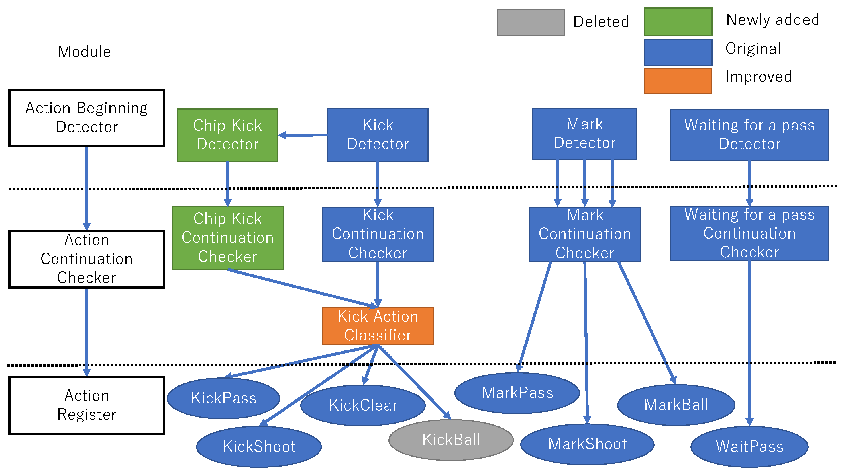
This section presents the results of experiments conducted to validate our proposed method. The validation is divided into two parts: clustering performance and online feasibility. The former evaluates offline clustering by both the Rand Index (RI) [13] and Adjusted Rand Index (ARI) [14] to confirm the effect on clustering performance when changing the data set. The latter assesses the feasibility of online clustering by the reduction ratio of the data set, the precision, and the convergence time.

3.1. Offline Clustering

Offline clustering in this paper is defined as clustering of logged data after the game, which means that we can exploit all geometric data broadcasted by SSL-Vision during the game. Action sequences can be extracted from the data in any duration, and all of them are used for clustering. To consider the duration for clustering strategies, set-plays such as throw-ins and corner kicks tend to represent some kinds of typical patterns. It can be considered that the set-plays are easier to cluster by a human than the other plays. From this viewpoint, we focus on clustering set-plays.
We used actual and test data for evaluation. Actual data were logged in the official SSL games of RoboCup 2015 and 2016. In general, there can be some noise and missing parts in the actual data. For a preliminary test before evaluating clustering of actual data, we created test data without any noise or missing parts. The test data were composed of 15 plays X 1 , X 2 , , X 15 that belong to three strategies as follows:
X 1 , X 4 , X 7 , X 10 , X 13 S I ; X 2 , X 5 , X 8 , X 11 , X 14 S II ; X 3 , X 6 , X 9 , X 12 , X 15 S III ,
where S I , S II , and S III stand for shoot after passing from a corner to the far side (Figure 5a), shoot after passing from a corner to the near side (Figure 5b), and shoot after passing from a corner to the near center circle (Figure 5c), respectively.
If the proposed method works ideally, each play should be grouped into the corresponding strategy.
By using the Rand Index (RI) [13] and Adjusted Rand Index (ARI) [14], the clustered result is evaluated in comparison with the ground truth. Note that:
  • the ground truth for logged data is the result given by the authors’ human clustering;
  • the ground truth for test data is obvious as explained in the last paragraph.
This comparative evaluation means whether or not the proposed algorithm can cluster plays as well as a human does. RI and ARI are well-known performance indexes for clustering. If the value of each index is one, it means that the clustered result matches the ground truth. In related work [4], RI is used for the performance index. For performance comparison with the method in [4], we adopt RI here as well; we give another evaluation based on ARI because ARI overcomes a drawback of RI.
First, experiments using test data were performed with the parameters in Table 3 to evaluate the clustering performance of the proposed method in comparison with the previous method [6]. Note that the following conditions are adopted for a fair comparative evaluation:
  • The end of the set-play in the previous method [5,6] is changed to the one in the proposed method. See Table 1 for the difference between the two definitions.
  • Let the number of clusters n c be the same between both methods. That is to say, n c is not computed by solving Equation (14) but is set to be constant in the experiments described in this section.
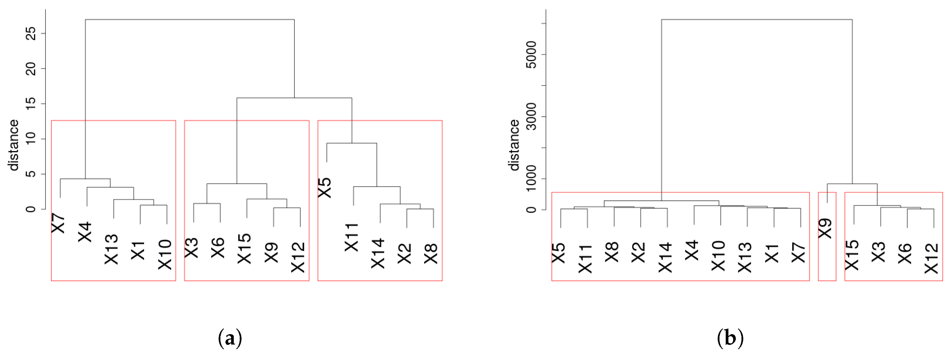
Figure 6 shows experimental results. Figure 6a is a dendrogram given by the proposed method; Figure 6b is a dendrogram given by the previous method in [6]. Strategies S I and S II are similar in terms of the trajectories of robots, but are different in terms of the trajectory of a ball. The previous method [6] cannot cluster these strategies separately. The reason for this is that a ball direction (or kick action) is not used as a feature for clustering in the previous method [6]. On the other hand, the proposed method achieves ideal clustering.
Next, by using logged data, we evaluate the proposed method in comparison with the previous method in [6]. The experimental conditions are the same as in the case of the test data. Table 4 summarizes the result. The proposed method is better than the previous one, especially for the values of ARI, which indicates that the proposed method using action sequences has the same or better performance than the previous method using geometric data, as in [6], despite the smaller amount of data.
Finally, we tested the proposed method with the number of clusters n c obtained from Equation (14). Table 5 shows the values of RI ranging from 0.835 to 0.943 (the average value: 0.885). From a comparison with Table 4, the difference of n c affects the result, but the performance is almost the same. In related work [4], the values of RI for some SSL games were reported. Focusing on only scenes close to our experimental settings (e.g., the number of set-plays), the values of RI range from 0.87 to 0.94 (average value: 0.907). This means that the performance of the proposed method is close to that of the method in [4].

3.2. Online Clustering

This subsection validates the online feasibility of the proposed method. Online clustering involves grouping an ongoing play into clusters successively during the game. In this type of clustering, the amount of data should be small to reduce storage space and also achieve fast computation. The clustered results would be useful for dominating the game against an opponent team.
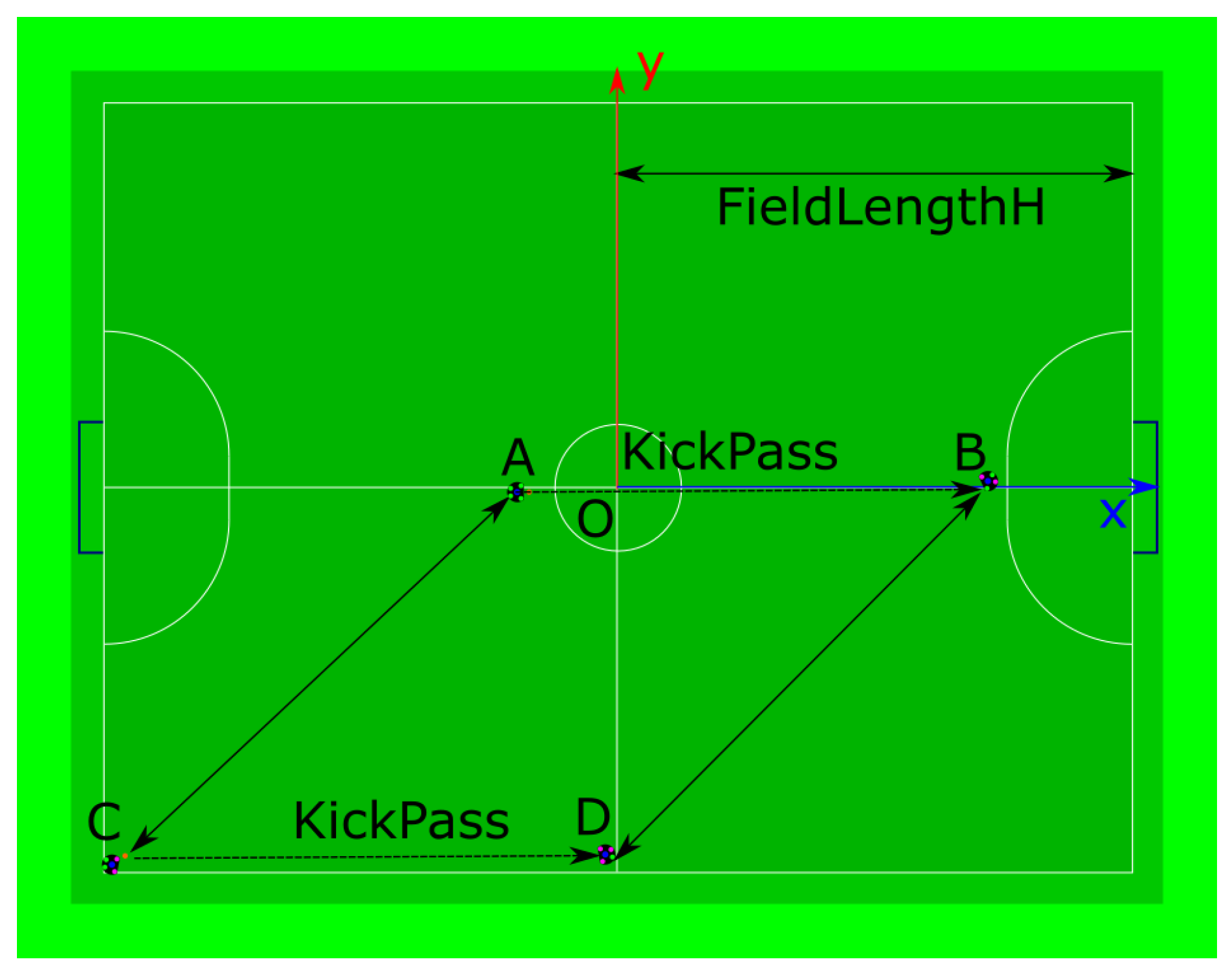
Regarding the amount of data for clustering, a method using action sequences has an advantage over one using geometric data. 
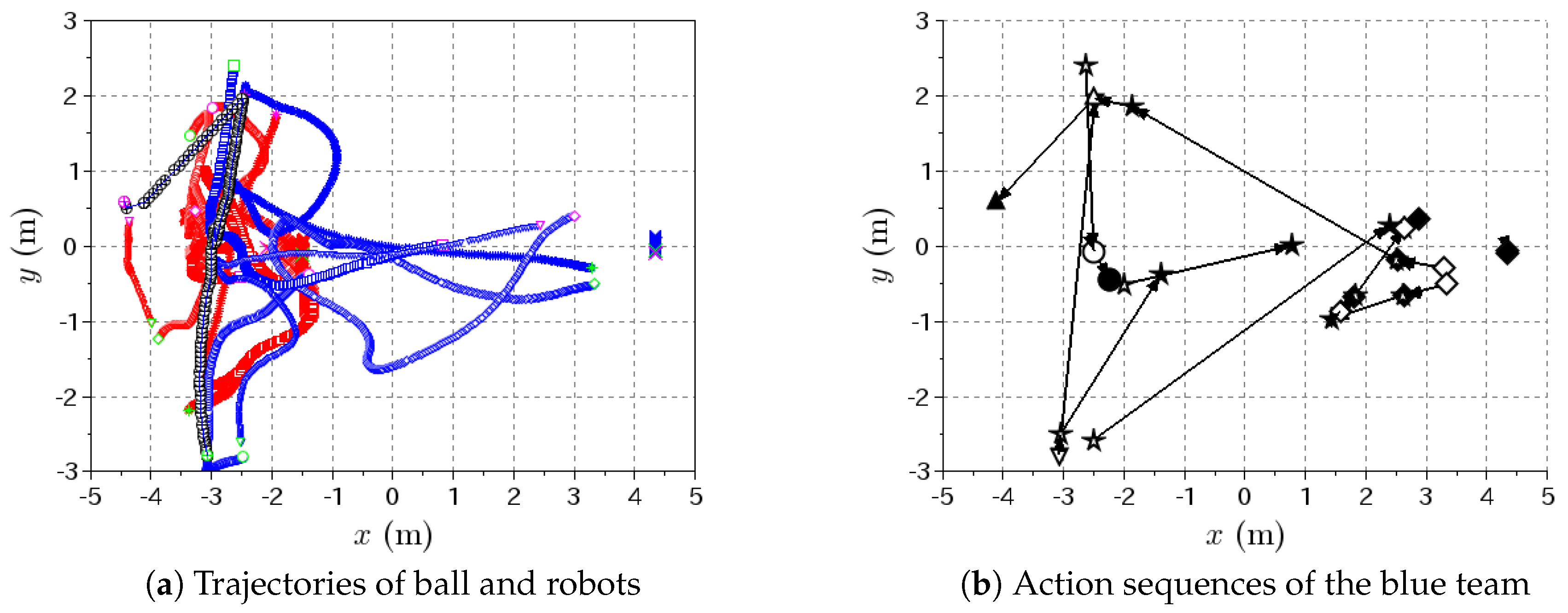
Figure 7 shows trajectories and corresponding action sequences in a set-play. Figure 7b depicts the action sequences extracted from the trajectories (i.e., geometric data) of the blue team in Figure 7a. The trajectories in Figure 7a are made up of 443 sampling data points expressed as ( x , y ) coordinates. If we use all coordinates of the blue team, the amount of data are 443 frames × 6 robots × 8 byte / coordinates = 21,264 byte , where a unit frame is defined as 1/60 s—the sampling period of SSL-Vision data. On the other hand, the action sequences in Figure 7b are made up of 15 actions, where the amount of data are 25 byte / action × 15 actions + 12 byte / play = 387 byte . In this case, the reduction ratio is (387/21,264) × 100 1.82 %, which means that action extraction compressed 98.18 % of geometric data. Table 6 shows the reduction ratios for several game logs from RoboCup 2015 and 2016. Note that these reduction ratios were averaged for the number of set-plays in each game. The results indicate that action extraction compresses the full geometric data to less than 2%.
Next, to evaluate the online performance of the proposed method, an experiment was conducted according to the following three steps: (i) analyzing the logged data every Δ c frames, (ii) arranging action sequences when the first kick of a play is detected, and (iii) evaluating the clustered results in comparison with the ground truth. Step (ii) is for adapting the current play to the previous ones. In Step (iii), the following precision is adopted as a performance index for clustering:
Precision = TP TP + FP ,
where TP and FP are defined as follows:
  • TP: the number of true positives, i.e., the number of plays that belong to both an inferred cluster and a true one.
  • FP: the number of false positives, i.e., the number of plays that belong not to an inferred cluster but to a true one.
Note that:
  • If the current play belongs to an inferred cluster, the precision with respect to the cluster can be computed. Otherwise, precision cannot be computed. This case is excluded from evaluation of precision.
  • Precision is computed every Δ c frames. The stored values are averaged not only per elapsed frame but also per play, as follows:
    1 n p n f p = 1 n p f = 1 n f Precision ,
    where p and f represent the numbers of plays and elapsed frames, respectively. Equation (18) is referred to as averaged precision in this paper.
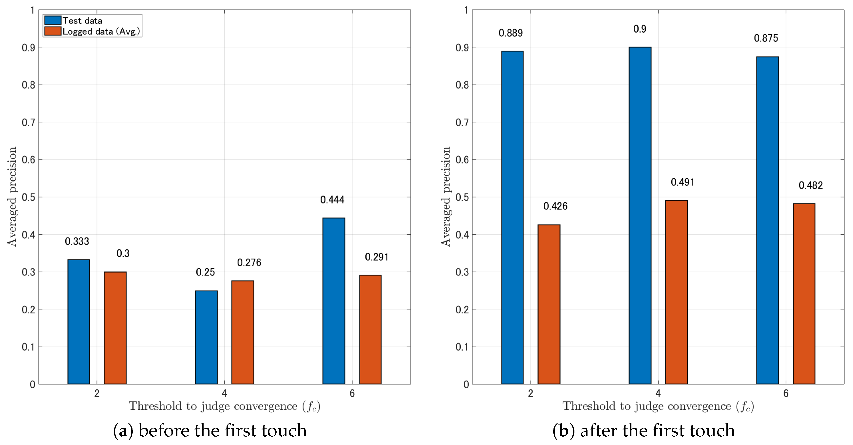
Additionally, how long it takes for the current play to converge into an inferred cluster is also important for online clustering. Such an elapsed period is referred to as f c . We here deal with three cases: f c = 2 , 4 , 6 .
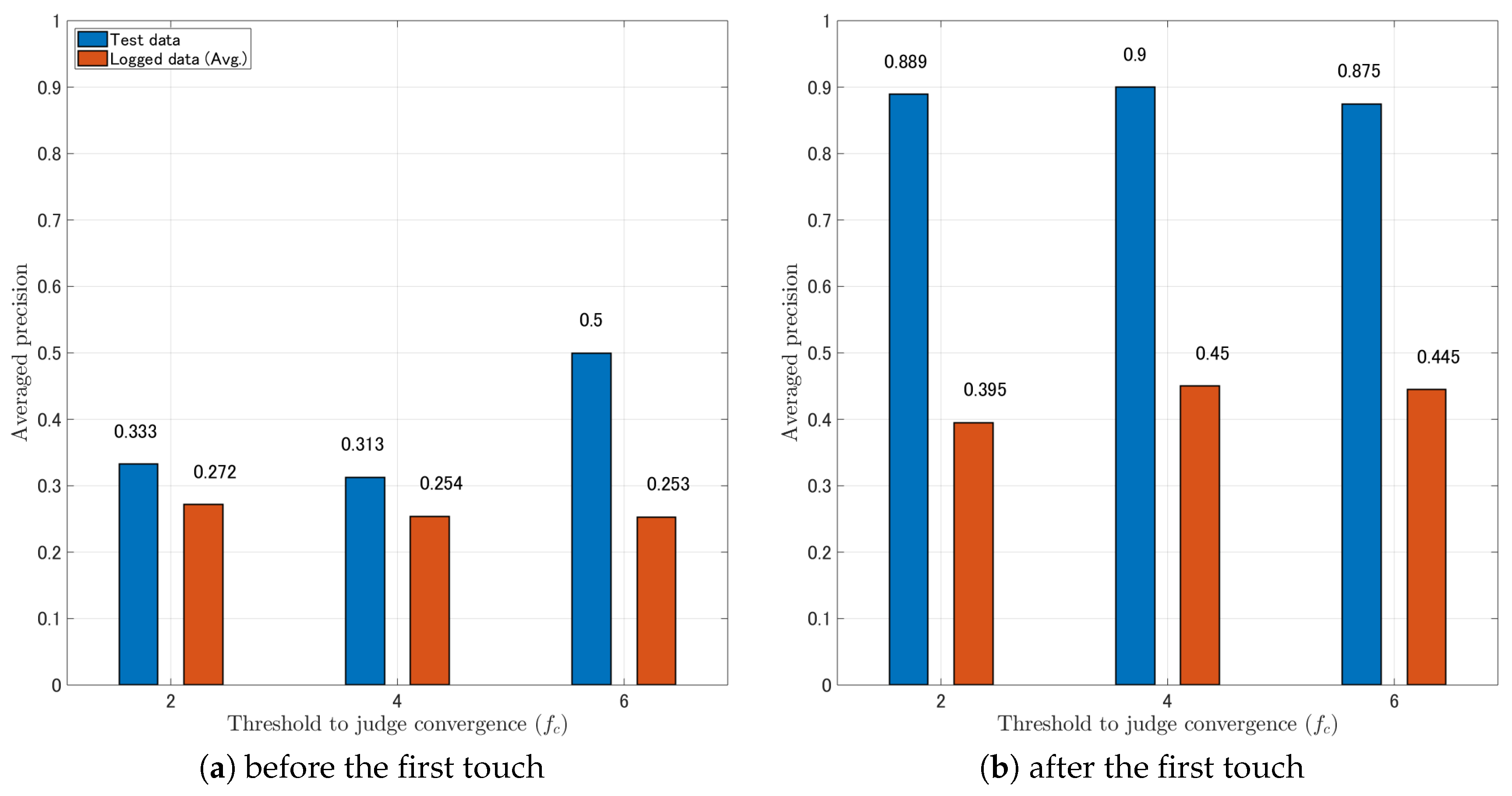
Any set-play can be divided into two phases by the first touch after restarting the game: one phase before the first touch and another phase after the first touch. In the phase before the first touch, the attacking team normally prepares for offense, e.g., coordinating the formation of the teammates according to a certain strategy. After one player of the attacking team touches the ball, the other players start their individual actions. Our objective is to estimate the strategy of the attacking team before the first touch or immediately after the first touch. For both the test data and logged data which are the same as in the previous subsection, Figure 8 shows the averaged precision. From the results in Figure 8, it can be seen that the averaged precision after the first touch is greater than the one before the first touch. This indicates that meaningful features of the strategy appeared since the first touch. In particular, regarding test data, the difference of averaged precision between before the first touch and after the first touch is quite large. This is because three kinds of strategies that compose the test data are similar before the first touch but totally differ after the first touch.
Table 7 shows the convergence time. Focusing on the results after the first touch, we can find the following relationship between the averaged precision in Figure 8 and convergence time in Table 7. The greater the value of f c becomes, the longer the convergence time is; the value of the averaged precision slightly grows from f c = 2 to f c = 4 while reducing from f c = 4 to f c = 6 . In particular, the result in the case of f c = 4 implies that the proposed algorithm used the correct strategy at 45% in less than half a second after the first touch.
The values of precision in Figure 8 were calculated by using all past set-plays in the cluster into which the ongoing set-play is grouped. We can also consider another way that involves picking the nearest play out of the cluster. The experimental results obtained in this way are depicted in Figure 10. By contrast with Figure 8, all values of precision are improved.

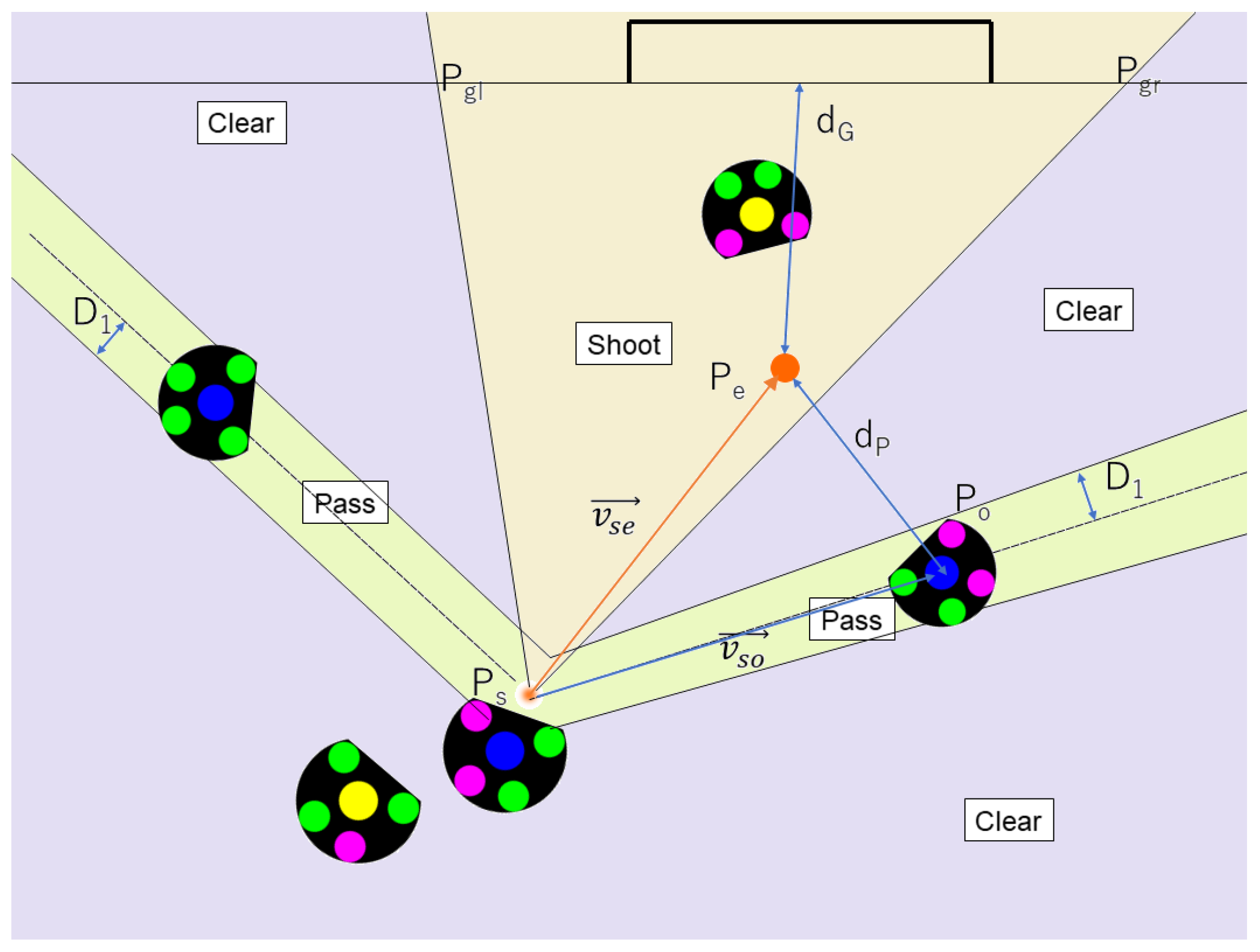
3.3. A Possible Application to Countering: Shoot-Cut

The proposed method can be applied to countering an opponent’s strategy. This subsection demonstrates shoot-cut as one defending strategy.
Numerical experiments were conducted on grSim [15]—an SSL simulator based on the Open Dynamics Engine (ODE). Four kinds of set-play strategies labeled S 1 , S 2 , S 3 , and S 4 were executed five times in this order. The strategies S 1 , S 2 , and S 3 are the same strategies used in test data named S I , S II , and S III , respectively. The S 4 is a new strategy including two passes and also is more complex than the other three strategies. Letting the obtained set-plays be referred as X 1 , X 2 , …, and X 20 , the relationship between them and S i is described as
X i , X i + 4 , X i + 8 , X i + 12 , X i + 16 S i , i = 1 , 2 , 3 , 4 .
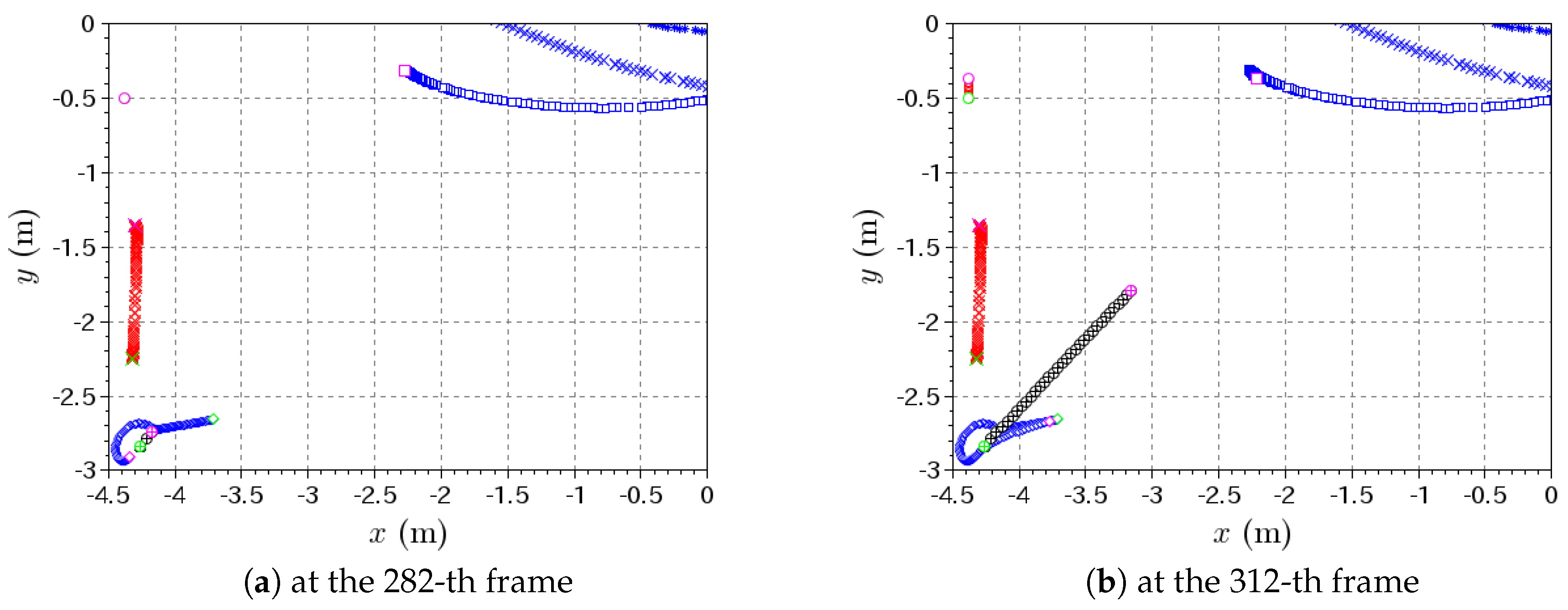
Figure 12 represents situations of set-plays X 4 and X 8 in a part of the field. There is a goal mouth located from ( 4.5 m , 0.5 m ) to ( 4.5 m , 0.5 m ) . At the beginning of a set-play, a goalkeeper and a defender of a defending team are placed at ( 4.4 m , 0.5 m ) and ( 4.3 m , 2.3 m ) , respectively; an attacking team deploys two players at ( 3.7 m , 2.7 m ) , and ( 1.5 m , 0.3 m ) , respectively. After restarting the game, the first touch is a kick by an attacker at ( 4.3 m , 2.9 m ) for passing a ball to another attacker at ( 2.3 m , 0.3 m ) . Then, the second attacker passes the ball to the first attacker again. Finally, the first attacker shoots the ball towards the goal of the defending team.
From Figure 12a, it can be seen that a defender did almost nothing against a shot ball from an attacking player at ( 2.7 m , 2.8 m ) . The reason is that X 4 was the first set-play from Strategy S 4 . On the other hand, Figure 12b shows that a defender tried to cut a shot ball. This means that a countering action of the defender was improved as a result of the increased number of stored set-plays from the same strategy. In addition, an action “KickShoot” can be easily found from the past action sequences that are most similar to the current action sequences.

4. Further Discussion on Online Strategy Clustering

In the previous section, the basic validity of the proposed method was demonstrated. Regarding online strategy clustering by the proposed method, this section gives a physical interpretation of the current performance and then considers further improvements.
Reconsider the result in Section 3.3 by taking the convergence time in Table 7 into account. According to Table 7, in the case of f c = 4 after the first touch, the convergence time is 0.476 s (=28.56 frames). This corresponds to the ball kicked at the first touch moving 1.428 m if the moving speed is 3 m/s. This situation can be applied to a set-play X 8 presented in Section 3.3. Figure 13 shows two situations in X 8 . The first touch after restarting the game was detected at the 282-th frame as shown in Figure 13a. The above convergence time is equivalent to about 30 frames. Figure 13b depicts a situation when 30 frames passed after the first touch. The situation represents that the ball is half way through the first pass. If an opponent’s strategy is identified at this moment, a defender will be able to behave somehow for countering it.
The proposed method would become more practical if accurate clustering is completed earlier. Figure 8 and Figure 10 show that the averaged precision before the first touch is lower than that after the first touch. This implies that actions before the first touch do not have enough information to identify a strategy behind the on-going set-play. To compensate for the weakness of action-based clustering, we can combine the proposed method with the method in [5,6], which focuses on a certain kind of geometric data, namely, deployment, before the first touch. That is to say, we can employ the following hybrid approach: deployment-based clustering before the first touch and then action-based clustering after the first touch.

5. Conclusions

This paper has proposed a strategy clustering method based on action sequences in the RoboCupSoccer SSL. In particular, the proposed method works not only offline but also online. The validity of the proposed method was experimentally confirmed from the viewpoints of clustering performance and online feasibility. The main findings are as follows:
  • The proposed method needs only 2% of the clustering data required by one of the previous methods (based on geometric data).
  • If there exist inferred categories, a set-play is grouped into an appropriate category at about 50% in 0.476 s since the first touch after restarting the game.
  • The proposed method can be used for performing a countering action to an opponent’s strategy.
In this paper, we used seven kinds of actions (KickShoot, KickPass, KickClear, MarkShoot, MarkPass, MarkBall, and WaitPass) for strategy clustering. However, we need to investigate which action mainly contributes to the clustered result. To achieve it, principal component analysis could be useful. On the other hand, there is still freedom in defining dissimilarity for improving the clustering performance (precision) and computational speed. As for this point, a deep neural network might give some hints. In addition, we will implement our proposed method in an actual SSL game to respond to opponent’s strategies, which would provide new aspects and findings.

Author Contributions

Conceptualization, Y.A.; methodology, Y.A., M.I. and T.N.; software, Y.A.; validation, Y.A., M.I. and T.N.; formal analysis, Y.A.; investigation, Y.A.; resources, M.I. and T.N.; data curation, Y.A.; writing—original draft preparation, Y.A.; writing—review and editing, M.I. and T.N.; visualization, Y.A.; supervision, M.I. and T.N.; project administration, M.I. and T.N.; funding acquisition, M.I. and T.N.

Funding

This work was supported by the Hibi Science Foundation, JSPS KAKENHI Grant No. JP16K00430, and Aichi Prefectural University.

Acknowledgments

The authors would like to thank all human and robot members of RoboDragons for their support.

Conflicts of Interest

The authors declare no conflict of interest.

Abbreviations

The following abbreviations are used in this manuscript:
SSLSmall Size League
RIRand Index
ARIAdjusted Rand Index

References

  1. RoboCup Federation RoboCup Federation Official Website. Available online: http://www.robocup.org/objective (accessed on 25 April 2019).
  2. Zickler, S.; Laue, T.; Birbach, O.; Wongphati, M.; Veloso, M. SSL-Vision: The Shared Vision System for the RoboCup Small Size League. In RoboCup 2009: Robot Soccer World Cup XIII. RoboCup 2009; Baltes, J., Lagoudakis, M.G., Naruse, T., Ghidary, S.S., Eds.; Lecture Notes in Computer Science; Springer: Berlin/Heidelberg, Germany, 2010; Volume 5949. [Google Scholar]
  3. Quintero, C.; Rodríguez, S.; Pérez, K.; López, J.; Rojas, E.; Calderón, J. Learning Soccer Drills for the Small Size League of RoboCup. In RoboCup 2014: Robot World Cup XVIII. RoboCup 2014; Lecture Notes in Computer Science; Springer: Cham, Switzerland, 2015; Volume 8992. [Google Scholar]
  4. Erdogan, C.; Veloso, M. Action selection via learning behavior patterns in multi-robot domains. In Proceedings of the International Joint Conference on Artificial Intelligence 2011, Barcelona, Spain, 16–22 July 2011; pp. 192–197. [Google Scholar]
  5. Yasui, K.; Kobayashi, K.; Murakami, K.; Naruse, T. Analyzing and Learning an Opponent’s Strategies in the RoboCup Small Size League. In RoboCup 2013: Robot World Cup XVII. RoboCup 2013; Behnke, S., Veloso, M., Visser, A., Xiong, R., Eds.; Lecture Notes in Computer Science; Springer: Berlin/Heidelberg, Germany, 2014; Volume 8371. [Google Scholar]
  6. Yasui, K.; Ito, M.; Naruse, T. Classifying an opponent’s behaviors for real-time learning in the RoboCup small size league. IEICE Trans. Inf. Syst. 2014, J97-D, 1297–1306. (In Japanese) [Google Scholar]
  7. Asano, K.; Murakami, K.; Naruse, T. Detection of Basic Behaviors in Logged Data in RoboCup Small Size League. In RoboCup 2008: Robot Soccer World Cup XII. RoboCup 2008; Iocchi, L., Matsubara, H., Weitzenfeld, A., Zhou, C., Eds.; Lecture Notes in Computer Science; Springer: Berlin/Heidelberg, Germany, 2009; Volume 5399. [Google Scholar]
  8. Adachi, Y.; Ito, M.; Naruse, T. Classifying the Strategies of an Opponent Team Based on a Sequence of Actions in the RoboCup SSL. In RoboCup 2016: Robot World Cup XX. RoboCup 2016; Behnke, S., Sheh, R., Sariel, S., Lee, D., Eds.; Lecture Notes in Computer Science; Springer: Cham, Switzerland, 2017; Volume 9776. [Google Scholar]
  9. Yasui, K.; Murakami, K.; Naruse, T. A New Detection Method of Kick Actions from Logged Data of SSL Games; JSAI Technical Report SIG-Challenge-B201-6; The Japanese Society for Artificial Intelligence (JSAI): Tokyo, Japan, 2012. (In Japanese) [Google Scholar]
  10. Rojas, R.; Simon, M.; Tenchio, O. Parabolic Flight Reconstruction from Multiple Images from a Single Camera in General Position. In RoboCup 2006: Robot Soccer World Cup X. RoboCup 2006; Lakemeyer, G., Sklar, E., Sorrenti, D.G., Takahashi, T., Eds.; Lecture Notes in Computer Science; Springer: Berlin/Heidelberg, Germany, 2007; Volume 4434. [Google Scholar]
  11. Weitzenfeld, A.; Biswas, J.; Akar, M.; Sukvichai, K. RoboCup Small-Size League: Past, Present and Future. In RoboCup 2014: Robot World Cup XVIII. RoboCup 2014; Bianchi, R., Akin, H., Ramamoorthy, S., Sugiura, K., Eds.; Lecture Notes in Computer Science; Springer: Cham, Switzerland, 2015; Volume 8992. [Google Scholar]
  12. Ito, M.; Suzuki, R.; Isokawa, S.; Du, J.; Suzuki, R.; Nakayama, M.; Ando, Y.; Umeda, Y.; Ono, Y.; Kashiwamori, F.; et al. RoboDragons 2019 Extended Team Description. RoboCupSoccer Small Size League. 2019. Available online: https://ssl.robocup.org/wp-content/uploads/2019/03/2019_ETDP_RoboDragons.pdf (accessed on 2 June 2019).
  13. Rand, W.M. Objective criteria for the evaluation of clustering methods. J. Am. Stat. Assoc. 1971, 66, 846–850. [Google Scholar] [CrossRef]
  14. Hubert, L.; Arabie, P. Comparing partitions. J. Classif. 1985, 2, 193–218. [Google Scholar] [CrossRef]
  15. Monajjemi, V.; Koochakzadeh, A.; Ghidary, S.S. grSim—RoboCup Small Size Robot Soccer Simulator. In RoboCup 2011: Robot Soccer World Cup XV. RoboCup 2011; Springer: Berlin/Heidelberg, Germany, 2012; pp. 450–460. [Google Scholar]
Figure 1. A brief flow of action extraction. The blue and orange boxes are submodules originally developed in [8]. The green boxes are submodules newly added in this paper. The orange submodules are improved in this paper. The oval objects represent extractable actions; the proposed algorithm does not use the gray one.
Robotics 08 00058 g001
Figure 2. Kick action classification in an example situation. Each framed box and its region indicate a kick category classified by the kick direction and P e ’s position. Note that “Kick” is omitted in the label here.
Robotics 08 00058 g002
Figure 3. The difference between trajectories of chip-kicked and normal-kicked balls in the image plane of the camera. P m ( m = 1 , 2 , ) represents a ball position sampled every frame between P s and P e ; P 0 corresponds to P s . See [11,12] for the structure of the robot with two types of kickers.
Robotics 08 00058 g003
Figure 4. A situation in which DistDiff takes the maximum value. When the distance between the starting and ending points of an action is longer than FieldLengthH, these actions are completely different, i.e., DistDiff = 1.
Robotics 08 00058 g004
Figure 5. Examples based on three types of strategies in test data. Blue, red, and black markers represent defending robots, attacking robots, and a ball, respectively. The green and magenta markers indicate the starting points and ending points of the trajectories, respectively.
Robotics 08 00058 g005
Figure 6. Dendrograms for the test data. (a) the proposed method; (b) the method in [6].
Robotics 08 00058 g006
Figure 7. Trajectories and action sequences of a set-play. In (a), blue, red, and black trajectories show a defending team, an attacking team, and the ball. The green and magenta markers indicate the starting points and ending points of the trajectories, respectively. In (b), markers indicate kinds of actions; the outline marker is the starting point and the other one is the ending point.
Robotics 08 00058 g007
Figure 8. Averaged precision for test data and logged data. See Figure 9 for averaged precision of individual logged data.
Robotics 08 00058 g008
Figure 9. Averaged precision for each team. Each precision is calculated by using all elements in the cluster in which the ongoing set-play is grouped. Their averaged precisions are shown in Figure 8.
Robotics 08 00058 g009
Figure 10. Averaged precisions for test data and logged data. In this case, only the nearest play in the cluster is used for the precision calculation. Averaged precisions for test data and logged data. See Figure 11 for averaged precision of individual logged data.
Robotics 08 00058 g010
Figure 11. Averaged precision for each team. Each precision is calculated by using the nearest set-play in the cluster in which ongoing set-play is grouped. Their averaged precisions are shown in Figure 10.
Robotics 08 00058 g011
Figure 12. The motion of defending robots (in red) against a ball (in black) moving among the attacking robots (in blue). The green and magenta markers indicate the starting points and ending points of the trajectories, respectively. The ball kicked at the bottom left corner was passed at ( 2.3 m, 0.3 m) and shot at ( 2.7 m, 2.8 m) towards the goal.
Robotics 08 00058 g012
Figure 13. Two situations in X 8 of Figure 12b. (a) an attacking robot has kicked a ball, then (b) 30 frames passed.
Robotics 08 00058 g013
Table 1. Comparison of the proposed method and previous methods [4,5,8].
MethodEnd of Set-PlayTarget ObjectData SetOnline Clustering
In this paperthe ball goes out of field or is intercepted by an opponentall opponentsactionpossible
In [8]the ball goes out of the field or is intercepted by an opponentall opponentsactionimpossible
In [5,6]the first kickall opponentsdeploymentpossible
In [4]the ball goes out of field or is intercepted by an opponentattacking opponentstrajectorypossible
Table 2. List of symbols.
SymbolsDescription
kick kick label indicating one of KickShoot, KickPass, and KickClear
P s , P e starting and ending points of ball’s trajectory
P o center point of the opponent who is the closest to pass line
v s e vector from P s to P e
e s e normalized vector of v s e
v s o vector from P s to P o
P g l , P g r left and right sides of our goal point, including margin
d G distance between P e and the center of the goal mouth
d P distance between P e and P o
D 1 parameter to express a region of Pass, like the thickness of the line through P s and P o
P m m-th point of the stored ball points
v s m vector from P s to P m
aaction label
KickSet action label set of kick actions {KickShoot, KickPass, KickClear}
i A p [ k ] k-th action by robot i in play p
i a p [ k ] k-th action label by robot i in play p
i s p [ k ] starting position vector of k-th action in play p
i e p [ k ] ending position vector of k-th action in play p
i A p action sequence of robot i in play p
A p action sequences which indicates play p
d 0 dissimilarity between actions
ActDiff dissimilarity indicating difference between action labels
AngDiff dissimilarity indicating difference between angles
DistDiff dissimilarity indicating difference between distances
d 1 dissimilarity between action sequences
k 2 s , k 2 e search range, start and end of the action sequence
LengthDiff dissimilarity indicating difference between lengths of each action sequence
KickUnuse additional dissimilarity corresponding to unused kicks
d 2 dissimilarity between plays
n c number of clusters
n p number of plays
n r number of robots
n f number of frames in a play
f c number of counts that the current play is sequentially grouped into the same cluster every Δ c  frames (See Table 3 for the definition of Δ c )
X i i-th set-play
S i i-th strategy
Table 3. Parameters in experiments.
ParameterMeaningValue(s)
TH p distance threshold for extracting a passer to mark400 mm
TH s distance threshold for extracting a shooter to mark400 mm
TH b distance threshold for extracting a ball-possessing player to mark400 mm
α b , β b weights in a criterion for extracting a ball-possessing player to mark 1 / 2 , 1 / 2
TH w angle threshold for extracting a player waiting for a pass 2 π / 45  rad
(=8 deg)
nnumber of frames for smoothing (for marking and waiting for a pass)3
N n a frame threshold for cutting off noise in making action sequences6 frames
(= 0.1  s)
N i a frame period for integrating the same kind of kick at the Action Register60 frames
(= 1.0  s)
α , β , γ weights for ActDiff, AngDiff, DistDiff in d 0 α = β = γ = 1 / 3
δ weight for LengthDiff in d 1 0.25
ϵ weight for KickUnuse in d 1 1.0
hthreshold for dividing clusters0.07
FieldLengthH half length of the field4500 mm
Δ c clustering period6 frames
Table 4. Clustering performance comparison between the proposed method and the previous method in [6]. The numbers of clusters are the same between the two methods. RI and ARI stand for the Rand Index and Adjusted Rand Index, respectively.
Target TeamThe Proposed MethodThe Method in [6]
RIARIRIARI
Test data110.7240.441
RoboFEI (vs. RoboDragons)0.8420.4070.8230.234
MRL (vs. RoboDragons)0.9240.7620.8950.647
STOX’s (vs. RoboDragons)0.8870.5270.8470.305
CMDragons (vs. RoboDragons)0.8020.1930.8570.399
ZJUNlict (vs. RoboDragons)0.8620.4090.8590.340
RoboDragons (vs. RoboFEI)0.9430.5950.9050.235
RoboDragons (vs. MRL)0.8920.2280.9050.216
RoboDragons (vs. STOX’s)0.8480.2980.8650.185
Average (without test data)0.8750.4270.8700.320
Table 5. Clustering performance of the proposed method. The number of clusters is obtained from Equation (14).
Target TeamRIARI
RoboFEI (vs. RoboDragons)0.8770.460
MRL (vs. RoboDragons)0.8760.535
STOX’s (vs. RoboDragons)0.8870.527
CMDragons (vs. RoboDragons)0.8350.259
ZJUNlict (vs. RoboDragons)0.8640.425
RoboDragons (vs. RoboFEI)0.9430.595
RoboDragons (vs. MRL)0.8830.208
RoboDragons (vs. STOX’s)0.9120.468
Average0.8850.435
Table 6. Reduction ratio of the amount of data by action extraction.
TeamsReduction Ratio (%)
Test data1.685
RoboFEI (vs. RoboDragons)1.444
MRL (vs. RoboDragons)1.370
STOX’s (vs. RoboDragons)1.248
CMDragons (vs. RoboDragons)1.831
ZJUNlict (vs. RoboDragons)1.864
RoboDragons (vs. RoboFEI)1.495
RoboDragons (vs. MRL)1.970
RoboDragons (vs. STOX’s)1.628
Average (without test data)1.606
Table 7. Averaged convergence time for test data and logged data. Note that the convergence time is measured from the first touch.
Type of DataAveraged Convergence Time (s)
Before the First TouchAfter the First Touch
f c = 2 f c = 4 f c = 6 f c = 2 f c = 4 f c = 6
Test data 3.577 3.315 2.700 0.1620.3770.573
Logged data (Average) 4.756 4.336 3.827 0.1670.4760.773

