Trajectory Design for Energy Savings in Redundant Robotic Cells ^†

Abstract

This work explores the possibility of exploiting kinematic redundancy as a tool to enhance the energetic performance of a robotic cell. The test case under consideration comprises a three-degree-of-freedom Selective Compliance Assembly Robot Arm (SCARA) robot and an additional linear unit that is used to move the workpiece during a pick and place operation. The trajectory design is based on a spline interpolation of a sequence of via-points: The corresponding motion of the joints is used to evaluate, through the use of an inverse dynamic model, the actuators effort and the associated power consumption by the robot and by the linear unit. Numerical results confirm that the suggested method can improve both the execution time and the overall energetic efficiency of the cell.

1. Introduction

The efficient use of resources is one of the challenges that industry has to face, not only to reduce the manufacturing and handling costs, but also to comply with the directives set by the European Union [1,2]. Such directives, which encourage the adoption of energy efficiency improvements, provide a strong market pull for energy-efficiency enabling technologies and research activities. The latter are testified by the flourishing literature [3] on the topic. Some recent theoretical [4] and experimental [5] investigations have shown that software and hardware solutions can lead to up to a 30% energetic improvement for robotic systems.

The work [3] proposes a classification of the numerous solutions proposed for the energetic improvement of automatic and and robotic systems. The classification identifies lightweight robot design [6], energy recovery and storage [7], robot architecture selection [8] and motion planning [9,10] as the main tools for achieving sensible energy consumption mitigation of automatic machines. Facing the problem of enhancing energetic efficiency by focusing on motion design has the advantage of being a ’software solution’ that can be applied to a wide range of systems. Not only are industrial robots the subject of studies on energy efficiency, since energy-saving trajectories for mobile robots are under investigation as well [11,12].

The impact of motion planning on the energy consumption of electric-driven mechatronic devices is well known and well understood, having been analyzed since the 1970s [13]. Several works have shown that simple analytical models can be effectively used to evaluate and optimize the power consumption of automatic machines [14,15]. These models can be used to formulate optimization problems that can be solved analytically for simpler cases or numerically for more complex ones [16].

Another tool that can be effectively exploited when designing energy-efficient motion profiles is kinematic redundancy, i.e., the availability of extra degrees of freedom of the robotic system [17]. Redundancy provides additional degrees of freedom to the solution of the inverse kinematic problem as well as to the choice of the motion profiles of the extra degrees of freedom. Increasing the number of degrees of freedom allows also to define a more energy efficient torque distribution among the actuators, as demonstrated for parallel robots in [18,19,20,21]. The work [18] analyzes several possible modifications to a planar kinematic robot, with the aim of finding the one that guarantees the higher energy savings, under a torque distribution managed by a predictive strategy. The numerical results are then extended to a full experimental validation in [19]. The optimal torque distribution in a redundantly actuated system can also be obtained by off-line optimization routines, as suggested in [20] or in [21].

This work suggest a novel approach to the topic of energy efficient operation of robots by discussing the optimization of the motion profiles for kinematically redundant robotic cells. This works proposes, as a test case, a robotic cell made by a three degrees of freedom (DOFs) Selective Compliance Assembly Robot Arm (SCARA) robot and a linear unit, which can be used to move the workpiece. Instead of introducing permanent modifications to the kinematics of an existing machine, as suggested in [18,19,20,21], here redundancy is introduced by adding an additional external and independent axis to a standard robot. A numerical optimization tool is suggested to fully exploit the availability of the extra degree of freedom through a careful design of the robot trajectory and of the motion design of the additional linear unit. The energy saving is then evaluated by comparing the result of the application of the proposed method with and without the use of the additional linear unit.

2. Energy Consumption Estimation

In this section the analytical models used for evaluating the energy consumption of the robotic cell is recalled. The goal is to find an expression for the energy consumption associated with a robotic task, which in this case is expressed as a trajectory in the operative space. Two models are presented, to describe separately the SCARA robot and the linear unit. For the second one, owing to its simpler dynamics, an analytic closed-form expression of the energy consumption will be presented.

2.1. SCARA Robot

The robotic cell used as a testbench comprises a three DOFs SCARA robot, as shown in Figure 1.

The SCARA robot is actuated by three brushless motors, and its main electric and mechanical parameters are reported in

Table 1. Mechanical and electric parameters of the Selective Compliance Assembly Robot Arm (SCARA) robot.

Parameter	Joint 1	Joint 2	Joint 3
Link length	0.45 m	0.35 m	-
Link mass	14 kg	18 kg	2 kg
Gear ratio	$1/30$	$1/30$	$1/30$
Motor inertia	$1\times {10}^{-4}$ kg m2	$1\times {10}^{-4}$ kg m2	$1\times {10}^{-4}$ kg m2
Viscous friction coefficient	0.001 Nm s/rad	0.001 Nm s/rad	0.001 Nm s / rad
Coulomb friction force	$2\times {10}^{-3}$ Nm	$2\times {10}^{-3}$ Nm	$2\times {10}^{-3}$ Nm
Motor winding resistance	3 Ω	3 Ω	3.5 Ω
Motor back-emf constant	0.6 Vs/rad	0.6 Vs/rad	0.6 Vs/rad
Motor torque constant	0.6 Nm/A	0.6 Nm/A	0.6 Nm/A
Peak motor torque	2.5 N	2.5 N	1.5 N
Peak motor power	75 W	75 W	50 W

. The dynamic model of the SCARA robot can be obtained by using the Lagrangian formalism, leading to the usual formulation:

$$\mathbf{M}\left(\mathbf{q}\right)\ddot{\mathbf{q}}+\mathbf{C}(\mathbf{q},\dot{\mathbf{q}})+{\mathbf{f}}_v\dot{\mathbf{q}}+{\mathbf{F}}_{c}sign\left(\dot{\mathbf{q}}\right)={\mathsf{\tau }}_m$$

(1)

Equation (1) involves the vector of joint coordinates $\mathbf{q}={\left[q_1,q_2,q_3\right]}^T$, the diagonal matrix ${\mathbf{f}}_v$ of viscous friction coefficients and the diagonal matrix of Coulomb friction forces ${\mathbf{F}}_c$. Motor torques at the joint are represented by the three components of vector ${\mathsf{\tau }}_m$. $\mathbf{M}\left(\mathbf{q}\right)$ is the configuration-dependent mass matrix, while $\mathbf{C}(\mathbf{q},\dot{\mathbf{q}})$ accounts for the centrifugal effects. The electromechanical model of the motors that drive the SCARA robot can be introduced into Equation (1), by recalling that the motor currents and the motor torques can be related by the diagonal matrix of the motor torque constants, ${\mathbf{k}}_t$, as:

$${\mathbf{\tau }}_m\left(t\right)={\mathbf{k}}_t\mathbf{I}\left(t\right)$$

(2)

The voltage drop across the motors can then be described by the equivalent DC motor armature model, which collects the contributions for all the joints of the robot:

$$\mathbf{V}\left(t\right)=\mathbf{R}\mathbf{I}\left(t\right)+\mathbf{L}{\displaystyle \frac{d\mathbf{I}\left(t\right)}{dt}}+{\mathbf{k}}_b{\dot{\mathbf{q}}}_m\left(t\right)$$

(3)

where ${\dot{\mathbf{q}}}_m$ is the vector of the motor velocities, ${\mathbf{k}}_b$ is the diagonal matrix of the motor back-emf constants, $\mathbf{R}$ is the matrix of motor winding resistances and $\mathbf{L}$ is the inductance matrix. The instantaneous power drawn by the robot is then simply expressed by the current-voltage product:

$${\mathbf{W}}_e\left(t\right)={\mathbf{V}}^T\left(t\right)\mathbf{I}\left(t\right)$$

(4)

If regenerative drives are assumed, and energy loss due to regeneration is neglected, the overall energy consumption for the time interval $[t_a,t_b]$ is found by computing the time integral:

$$E_{SCARA}={\int }_{t_a}^{t_b}{\mathbf{V}}^T\left(t\right)\mathbf{I}\left(t\right)dt$$

(5)

This model can be implemented within the trajectory optimization routine, which will include the numerical integration of Equation (5), following the approach commonly used in works such as [22]. It must be pointed out that the electric power, as expressed in Equation (4), takes positive values when the energy is drawn by the robot from the drive unit and negative values when the energy flow is reversed. Whenever the motor drives does not support regeneration [23], the current drawn from the actuators during the braking phase is dissipated by a braking resistor, and therefore negative values of ${\mathbf{P}}_e\left(t\right)$ should be not accounted for in Equation (5). Both the cases of regenerative and non-regenerative robot drives are taken into consideration in Section 3 to highlight the results of the energy optimization in both cases.

2.2. Linear Unit

The estimation of the energy needed to drive the fourth axis of the robotic cell, i.e., the sliding table, can be efficiently performed using an analytical closed-form formulation rather then by numerical integration, as imposed by the analytical complexity of the SCARA robot dynamics.

The dynamics of the linear unit can be described by a single differential equation, that takes the common form of the dynamics of a constant inertia systems, as:

$$m{\ddot{q}}_4\left(t\right)+f_v{\dot{q}}_4\left(t\right)+F_{c}sign\left({\dot{q}}_4\left(t\right)\right)=F_m\left(t\right)$$

(6)

The parameters appearing in Equation (6) are the moving mass of the linear unit m, the coefficient of viscous friction $f_v$ and the Coulomb friction force $F_c$. Since the linear unit is actuated in a direct drive arrangement, i.e., without the use of transmission system, the force acting on the moving mass is equal to the force $F_m\left(t\right)$ exerted by the brushless linear motor which drives the unit. If required, this formulation can be extended in a straightforward manner to include reversible transmission system, such as a ball screw mechanism. The values used to define the model of the linear unit are shown in

Table 2. Mechanical and electric parameters of the linear unit.

Parameter	Value
Moving mass	5.18 kg
Viscous friction coefficient	$1\times {10}^{-3}$ Ns/m
Coulomb friction force	$2\times {10}^{-2}$ N
Back-emf constant	3.1 Vs/m
Torque constant	3.12 N/A

.

The equations that describe the electric dynamics of the linear unit are the scalar equivalents of the ones already used for the robot, i.e., Equations (2) and (3). Accordingly, the instantaneous electric power drawn by the linear unit can be written as:

$$\begin{array}{cc}\hfill W_{LU}\left(t\right)=& {\displaystyle \frac{R}{k_t^2}}\left(m^2{\ddot{q}}_4^2\left(t\right)+f_v{\dot{q}}_4^2\left(t\right)+F_c^2+2m{f}_v{\dot{q}}_4\left(t\right){\ddot{q}}_4\left(t\right)+2f_v{F}_c{\dot{q}}_4\left(t\right)\right)\hfill \\ & +{\displaystyle \frac{k_b}{k_t}}\left(m{\dot{q}}_4\left(t\right){\ddot{q}}_4\left(t\right)+f_v{\dot{q}}_4^2\left(t\right)+F_c{\dot{q}}_4\left(t\right)\right)\hfill \end{array}$$

(7)

Equation (7) does not include the effects of inductance on power absorption, since they are negligible. Equation (7) shows that the instantaneous electric power drawn by the motor is the sum of a constant term, associated with the Coulomb friction force $F_c$, and of a term that depends on speed, acceleration, on their product and on their squared values. The time integration of Equation (7) over the interval $[0,T]$ results in the estimation of the energy required to perform a generic motion profile. In a rest-to-rest motion profiles the energy associated with the acceleration ${\ddot{q}}_4\left(t\right)$, with its squared value ${\ddot{q}}_4^2\left(t\right)$ and with the speed-acceleration product are null, i.e.,

$${\int }_0^T{\ddot{q}}_4\left(t\right)dt=0;{\int }_0^T{\ddot{q}}_4^2\left(t\right)dt=0;{\int }_0^T{\dot{q}}_4\left(t\right){\ddot{q}}_4\left(t\right)dt=0;$$

(8)

Furthermore, the power contribution that is directly proportional to the speed, when integrated, is simply related to the overall displacement H, given that:

$${\int }_0^T{\dot{q}}_4\left(t\right)dt=H$$

(9)

The overall energy consumption can therefore be rewritten by rearranging Equation (7) and by computing its definite integral over $[0,T]$ as:

$$\begin{array}{cc}\hfill E_{LU}=& \left({\displaystyle \frac{R}{k_t^2}}+{\displaystyle \frac{k_b}{k_t}}\right)f_v{\int }_0^T{\dot{q}}_4^2\left(t\right)dt+\left(2{\displaystyle \frac{R}{k_t^2}}{f}_v+{\displaystyle \frac{k_b}{k_t}}\right)F_{c}H\hfill \\ & +F_c{\displaystyle \frac{R}{k_t^2}}T+{\displaystyle \frac{R}{k_t^2}}{m}^2{\int }_0^T{\ddot{q}}_4^2\left(t\right)dt\hfill \end{array}$$

(10)

The formulation of Equation (10) can also be rearranged by highlighting the contributions proportional to the RMS value of joint speed ${\dot{q}}_4$ and acceleration ${\ddot{q}}_4$ using the formulas:

$$\begin{array}{cc}\hfill {\int }_0^T{\dot{q}}_4\left(t\right)dt& =T{\dot{q}}_{4,RMS}^2\hfill \end{array}$$

(11)

$$\begin{array}{cc}\hfill {\int }_0^T{\ddot{q}}_4\left(t\right)dt& =T{\ddot{q}}_{4,RMS}^2\hfill \end{array}$$

(12)

Accordingly, the energy used by the linear unit can be computed as the sum of four terms, highlighting the proportionality to the total displacement H, to the motion time T, to the root-means-square (RMS) values of speed and acceleration, as:

$$E_{LU}=\left({\displaystyle \frac{R}{k_t^2}}+{\displaystyle \frac{k_b}{k_t}}\right)f_{v}T{\dot{q}}_{4,RMS}^2+\left(2{\displaystyle \frac{R}{k_t^2}}{f}_v+{\displaystyle \frac{k_b}{k_t}}\right)F_{c}H+F_c{\displaystyle \frac{R}{k_t^2}}T+{\displaystyle \frac{R}{k_t^2}}{m}^{2}T{\ddot{q}}_{4,RMS}^2$$

(13)

Equation (13) is of general application, since it can be used for any choice of the rest-to-rest motion profile of the linear unit, provided that the the RMS values of the table speed and acceleration can be computed. As suggested in [24], their computation can be performed using the characteristic coefficients of RMS speed and acceleration, $c_{V_{RMS}}$ and $c_{A_{RMS}}$, which are commonly available in standard reference books [25]. Such coefficients are computed with reference to a normalized motion profile $q_N\left(\tau \right)$, which provides a unitary displacement over a unitary time duration, as:

$$\begin{array}{c}\hfill C_{v,RMS}=\sqrt{{\int }_0^T{\left({\displaystyle \frac{d{q}_N}{d\tau }}\right)}^{2}d\tau }\end{array}$$

(14)

$$\begin{array}{c}\hfill C_{a,RMS}=\sqrt{{\int }_0^T{\left({\displaystyle \frac{d^2{q}_N}{d{\tau }^2}}\right)}^{2}d\tau }\end{array}$$

(15)

Recalling that [24]:

$$\begin{array}{c}\hfill {\dot{q}}_{4,RMS}={\displaystyle \frac{H}{T}}{C}_{v,RMS}\end{array}$$

(16)

$$\begin{array}{c}\hfill {\ddot{q}}_{4,RMS}={\displaystyle \frac{H}{T^2}}{C}_{a,RMS}\end{array}$$

(17)

the total energy consumption of the linear unit while performing a generic rest-to-rest motion can be evaluated also as:

$$E_{LU}=\left({\displaystyle \frac{R}{k_t^2}}+{\displaystyle \frac{k_b}{k_t}}\right)f_{v}T{\left({\displaystyle \frac{h}{T}}{c}_{v,RMS}\right)}^2+\left(2{\displaystyle \frac{R}{k_t^2}}{f}_v+{\displaystyle \frac{k_b}{k_t}}\right)F_{c}H+F_c{\displaystyle \frac{R}{k_t^2}}T+{\displaystyle \frac{R}{k_t^2}}{m}^{2}T{\left({\displaystyle \frac{h}{T^2}}{c}_{a,RMS}\right)}^2$$

(18)

3. Energy Optimization

The energy consumption models reported in Section 2 can be used as the basis of an energy optimization problem. Countless choices are available as far as the trajectory primitive is concerned, according to the extensive results available in literature [25,26]. As a matter of example, in this work the trajectory design is performed with reference to the so-called ‘434’ spline algorithm. This motion profile, which was introduced by Cook and Ho in [27], is based on the use of piecewise polynomial functions as the means to produce a trajectory that passes through a sequence of via-points, which might be expressed either in the operative or in the joint space domain. The motion primitive takes its name from the sequence of third and fourth degree polynomials function that are used to provide the interpolation of the via-points with continuity up to the second derivative, so that continuous acceleration is always achieved. Further alterations of the original definition can be performed to achieve speed, acceleration and jerk limitations [28].

In the case under consideration in this work an energy saving trajectory design is sought, using the 434 trajectory for the SCARA robot, even if the method can be applied, with obvious modifications, with spline algorithms and with arbitrary motion profile of the linear unit. The task is specified by N via-points that are usually defined, for the operator’s convenience, in the operative space, meanwhile the computation of the interpolated motion profile according to the aforementioned 434 algorithm is performed after their transformation to the joint space.

This motion profile is used here also to exploit its simple parametrization: Once a sequence of via-points is defined, the trajectory is designed by setting the time distance between each two consecutive via-points. Each trajectory implementation is uniquely identified by a vector of time distances $\mathbf{T}$, which comprises $N-1$ elements, each one identified as $T_i$. This feature makes the ’434’ trajectory profile very suitable to be the basis of an optimization procedure.

As far as the optimization of the motion of the linear unit is concerned, here the ’symmetric double-S’ profile is chosen as the motion law, but the procedure can be adopted to other motion profiles using a similar procedure. The motion is conveniently described by the piecewise expression of the velocity as:

$$\begin{array}{ccc}{\dot{q}}_4\left(t\right)={\displaystyle \frac{v_0}{2}}\left(1-cos\left({\omega }_{1}t\right)\right);\hfill & \hfill & t\in [0,t_a)\hfill \\ {\dot{q}}_4\left(t\right)=v_0;\hfill & \hfill & t\in [t_a,T-t_a)\hfill \\ {\dot{q}}_4\left(t\right)={\displaystyle \frac{v_0}{2}}\left(1+cos\left({\omega }_{1}t\right)\right);\hfill & \hfill & t\in (T-t_a,T]\hfill \end{array}$$

(19)

with

$$v_0={\displaystyle \frac{H}{T-t_a}};{\omega }_1={\displaystyle \frac{\pi }{t_a}};$$

(20)

The motion of the linear unit is therefore split into three phases, comprising an acceleration and deceleration phase, each one lasting $t_a$ seconds, and a constant speed phase. Equation (20) ensures that the whole displacement H is performed in the total time T. If the total motion time T is prescribed, the optimization of the trajectory of the linear unit can be performed by setting the acceleration time $t_a$ within the range $(0,T/2]$. After evaluating the coefficients $c_{v,RMS}$ and $c_{a,RMS}$ according to Equations (19) and (20) and by using them into Equation (18), the energy consumption of the linear unit is:

$$E_{LU}=f_v\left({\displaystyle \frac{R}{k_t^2}}+{\displaystyle \frac{k_b}{k_t}}\right)\left(T-{\displaystyle \frac{5}{4}}{t}_a\right)v_0^2+\left({\displaystyle \frac{R}{k_t^2}}2f_v+{\displaystyle \frac{k_b}{k_t}}\right)F_{c}H+F_c{\displaystyle \frac{R}{k_t^2}}T+{\displaystyle \frac{R}{t_a}}{\left({\displaystyle \frac{m{v}_0}{2k_t}}\right)}^2$$

(21)

Equation (21) is written for the double-S motion profile, but it should be highlighted that the formulation of Equation (18) can be applied to any arbitrary motion profile, simply by finding the corresponding values for the characteristic coefficients $c_{v,RMS}$ and $c_{a,RMS}$.

Once a method for evaluating the energy consumption of the whole cell is established, a numerical optimization can be set up according to the following problem:

$$\begin{array}{cc}\hfill \underset{[\mathbf{T},t_a]}{min}& E_{SCARA}+E_{LU}\hfill \\ \hfill \mathrm{with}:& \mathbf{T}\in R^{N-1};\hfill \\ \hfill & t_a\in \left(0,T/2\right];\hfill \\ \hfill \mathrm{subject}\mathrm{to}:& {\displaystyle \sum _{i=1}^{N-1}}{T}_i=T;\hfill \\ \hfill \mathrm{bounded}& |\dot{\mathbf{q}}|,|\ddot{\mathbf{q}}|,|\stackrel{⃛}{\mathbf{q}}|;\hfill \\ \hfill \mathrm{bounded}& |W_{e,j}|,|{\tau }_j|,\mathrm{with}j=1,2,3;\hfill \end{array}$$

(22)

The cost function used in Equation (22) equally weighs the energy required by the robot and by the linear unit, therefore the optimization problem is targeted at reducing the overall energy consumption of the robotic cell. The energy required by the SCARA robot, $E_{SCARA}$ is evaluated according to Equations (2)–(5), while $E_{LU}$ is evaluated using just Equation (21). Optimization variables includes the set of $N-1$ times $T_i$ between two consecutive via-points, which are collected in the vector $\mathbf{T}$, and the acceleration time $t_a$, which sets the design of the motion profile of the linear unit according to Equations (19) and (20). The whole task is designed to be performed in T seconds, and the motion of both devices happens simultaneously and without any pauses. In addition to the bounds on absolute values joint speed, acceleration and jerk, the optimization problem in Equations (22) can account for limits on the peak values of the motor torques ${\tau }_j$ and on the electric power $W_{e,j}$ draw by the j-th motor. The last two constraints are enforced to ensure the limitation imposed by the robot drive unit.

The optimization problem is not convex, however a careful selection of the initial guess has shown to be capable of getting rid of this issue and to boost the achievement of significant energy reductions. A sensible initial guess for the starting value of the times $T_i$ can be obtained using either the chord length distribution or the centripetal distribution methods, as proposed in literature [25].

The benchmark problem taken into consideration in this work is described by six via-points defined in a reference frame located on the sliding table. The six via-points, which are reported in

Table 3. Coordinates of the via-points for the pick & place task.

Via-point	X [m]	Y [m]	Z [m]
1	0.6	0.2	0
2	0.6	0.2	0.2
3	0.6	0.2	0.3
4	−0.2	0.4	0.3
5	−0.2	0.4	0.2
6	−0.2	0.4	0

, reproduce a pick & place task that involves the motion of all the four axes of the robotic cell. This choice reproduces a typical task performed by SCARA robots in assembly or packaging applications. The energetic performance of the proposed method is measured in comparison with a non-redundant solution, the latter being obtained without the use of the linear unit, i.e., by enforcing ${\dot{q}}_4\left(t\right)=0$.

3.1. Trajectory Optimization with Electric Power Regeneration

Figure 2 reports the results of the solution of the optimization problem of Equation (22) for a sequence of execution times varying from $T=7$ s to $T=2$ s, halting the iteration when reducing the minimum time allowed by the constraints. The procedure was repeated for the redundant and the non-redundant task.

The solid line in Figure 2 shows the minimum energy required to perform the task in the redundant case, while the dashed line refers to the use of the SCARA robot only. In all the cases included in Figure 2 the redundant configuration is by a noticeable amount the most energetically efficient one. It can also be highlighted that the advantage in terms of energy saving allowed by the redundancy is more relevant for faster motion profiles.

The non-redundant configuration requires at best 20.5 J to complete the task, while just 13.6 J are needed when using the linear unit. Optimal execution times are 3.23 s and 2.25 s, respectively. Figure 3 and Figure 4 show the optimal trajectories as designed through the optimization routine.

In particular, Figure 3 shows the speed of each axis for the minimum energy solutions. It can be seen that the motion of joints 2 and 3 are radically different when switching from the redundant to the non-redundant configuration, since the motion along the X direction is in one case provided by the SCARA robot, and in the other one is provided by the linear unit. The frame of reference for the Cartesian motion of the end-effector is shown in Figure 1. Hence the SCARA robot performs a smaller displacement in the redundant case. The motion along the vertical direction, which is provided by the third axis, follows a similar profiles in both cases, with the noticeable difference of a sensibly shorter execution time in the redundant case due to the smaller optimal motion duration.

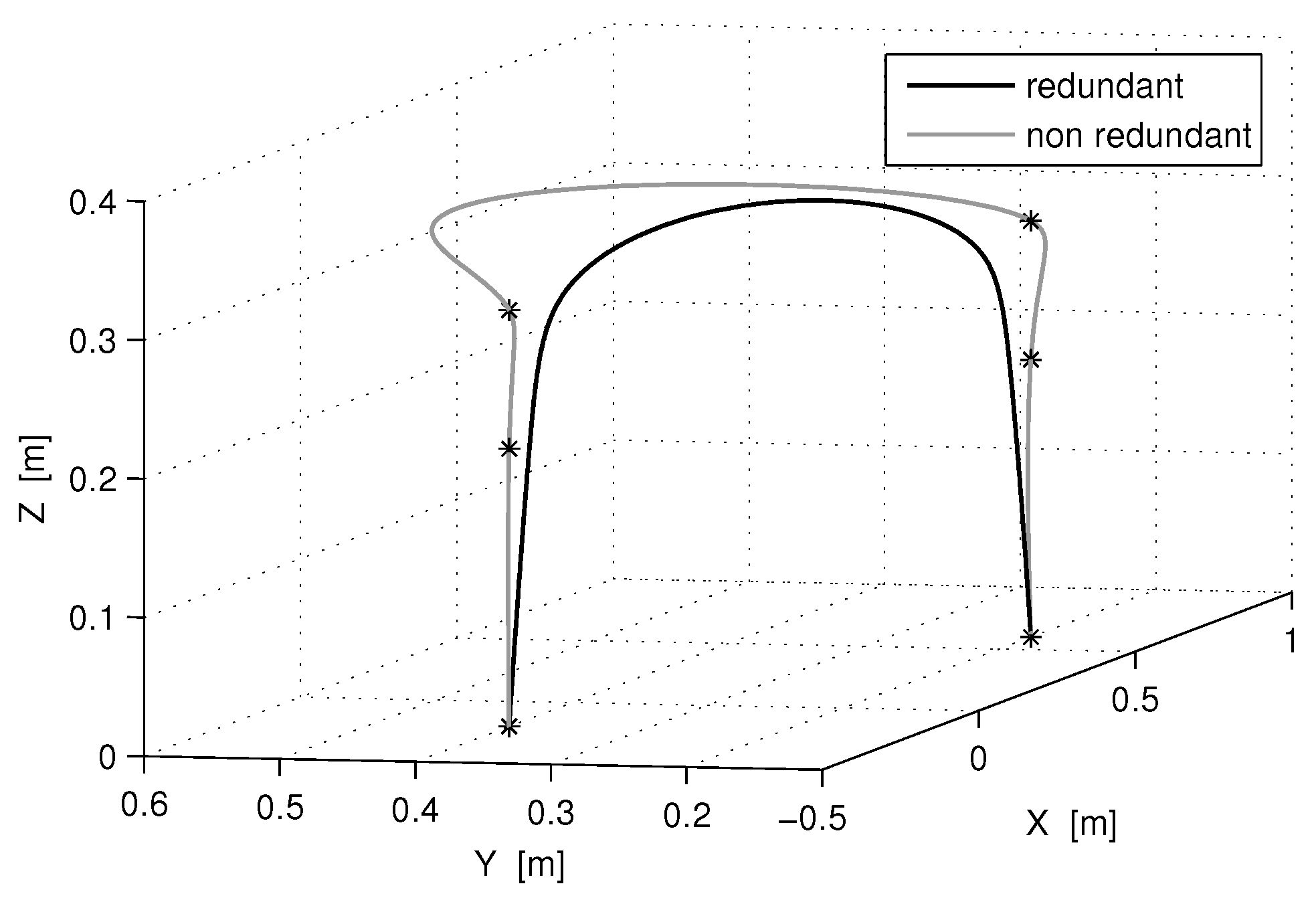
The corresponding paths of the SCARA end effector are shown in Figure 5: In the non-redundant case the motion of the end-effector passes exactly through all the six via-point, while in the redundant configuration just the first and the last via-points are touched by the path. The corresponding distortion of the path is due to the absence of a synchronization between the motion of the robot and of the linear unit, as the result of using a rest-to-rest motion profile for the linear unit and a via-point approach for the robot.

It is indeed worthwhile to notice that for the third joint, the peak speed values are essentially unaffected by the shorter execution time associated with the redundant configuration: Also the corresponding acceleration, as it can be seen in Figure 4, shows almost identical profiles of the first and the last segment of the trajectory. In all cases the peak values of speed, acceleration and, although not shown, jerk, are comfortably within the kinematic bounds imposed when defining the optimization procedure.

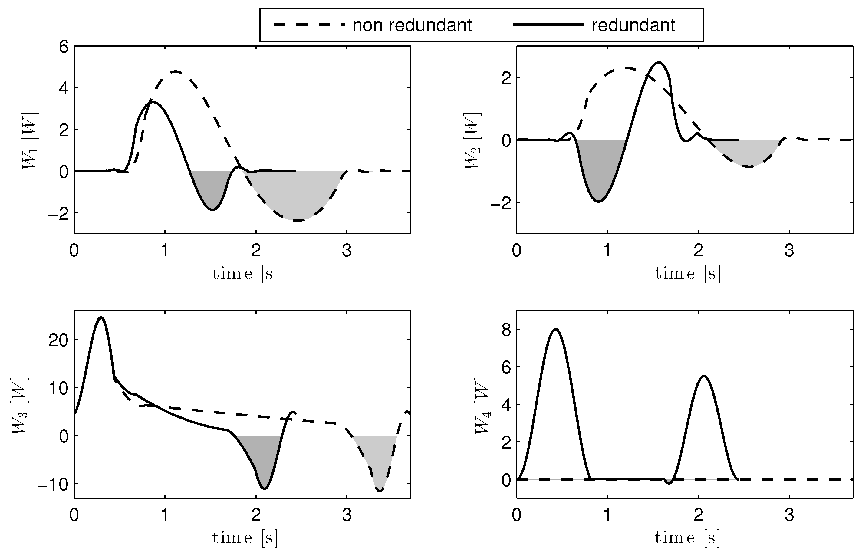
The profiles of the absorbed electric power obtained in the same tests are are reported in Figure 6. The dashed lines, which refer to the non-redundant configuration, shows that all the motors that drive the SCARA robot draw electric energy during the first half of the task, while a fraction of that energy is fed back to motor drives in the remaining part of the trajectory. The power profiles optimized for the redundant trajectory, which are represented by solid lines in Figure 6 has the interesting property of alternating energy absorption and energy regeneration phases between joints 1 and 2. The same figure shows that the amount of energy that can be regenerated by the fourth axis is negligible, given that the current regenerated during the braking phase by the linear unit is almost completely dissipated in the motor windings due to resistive losses.

3.2. Trajectory Optimization Without Regeneration

The trajectory design procedure has been repeated by taking into consideration the very same task, with the only difference being that is has been assumed that the drive circuit of the SCARA robot do not support energy regeneration. The iteration of the design procedure for total execution times that range from 7 to 2 s, results in the two energy vs. time profiles shown in Figure 7. As far as the overall energy consumption is concerned, the addition of the fourth axis does, again, offers the possibility of reducing the energy consumption and achieving a consistent speed-up.

The two energy-optimal solutions require 25.9 J and 16.9 J, with execution times equal to, respectively, 3.700 s and 2.442 s. The joint speed and acceleration profiles corresponding to the two optimal solutions are shown in Figure 8 and Figure 9. Comparing them to Figure 3 and Figure 4, which are generated under the full regeneration hypothesis, shows that the trajectories that lead to the energy optimality are very similar to each other. It can be inferred that, for the case under investigation, the energy regeneration has a minor effect on the trajectory design.

Figure 9 highlights that, accordingly to the results already presented in Figure 4, the timing of the motion of the linear unit that leads to the minimum energy consumption is the one that sets the acceleration and deceleration times equal to one third of the total execution time T.

Also the direct comparison between Figure 6 and Figure 10, which show the power absorption with and without regeneration highlights the similarity between the two profiles. The absence of regenerated energy is indicated in Figure 10 by shading the areas underlined by negative values of the absorbed electric power: The energy associated to such contributions will be dissipated on a braking resistor and therefore will not be accounted for when evaluating Equation (5).

The main difference between the optimal trajectories obtained with and without energy regeneration is that the latter requires a slightly longer execution time.

4. Conclusions

This works suggests a solution to the problem of designing optimal tasks for robotic cells by exploiting kinematic redundancy as a tool for improving the performance. The suggested method, applied to a robotic cell which comprises a SCARA robot and a linear unit used to move the workpiece, has been capable of producing motion profiles with a reduced energy consumption and a faster execution time in comparison to equivalent non-redundant configurations. Time speed-up and efficiency increase are achieved with and without the aid of regenerative braking. The trajectory optimization design is based on an inverse dynamic model of the robotic cell, which is used together with an analytical model of the energy consumption. The proposed method is of general application, since it can be applied to several other robotic architectures and to different motion profiles.

References

- Helm, D. The European framework for energy and climate policies. Energy Policy 2014, 64, 29–35. [Google Scholar] [CrossRef]
- Tanaka, K. Review of policies and measures for energy efficiency in industry sector. Energy policy 2011, 39, 6532–6550. [Google Scholar] [CrossRef]
- Carabin, G.; Wehrle, E.; Vidoni, R. A review on energy-saving optimization methods for robotic and automatic systems. Robotics 2017, 6, 39. [Google Scholar] [CrossRef]
- Hansen, C.; Eggers, K.; Kotlarski, J.; Ortmaier, T. Comparative evaluation of energy storage application in multi-axis servo systems. In Proceedings of the 14th IFToMM world congress, Taipei, Taiwan, 25–30 October 2015; pp. 201–210. [Google Scholar]
- Meike, D.; Ribickis, L. Energy efficient use of robotics in the automobile industry. In Proceedings of the 15th International Conference on Advanced Robotics (ICAR), Tallinn, Estonia, 20–23 June 2011; pp. 507–511. [Google Scholar]
- Kim, Y.J. Design of low inertia manipulator with high stiffness and strength using tension amplifying mechanisms. In Proceedings of the 2015 IEEE/RSJ International Conference on Intelligent Robots and Systems (IROS), Hamburg, Germany, 28 September–2 October 2015; pp. 5850–5856. [Google Scholar]
- Aziz, M.A.; Zhanibek, M.; Elsayed, A.S.; AbdulRazic, M.O.; Yahya, S.; Almurib, H.A.; Moghavvemi, M. Design and analysis of a proposed light weight three DOF planar industrial manipulator. In Proceedings of the IEEE Industry Applications Society Annual Meeting, Portland, OR, USA, 2–6 October 2016; pp. 1–7. [Google Scholar]
- Li, Y.; Bone, G.M. Are parallel manipulators more energy efficient? In Proceedings of the 2001 IEEE International Symposium on Computational Intelligence in Robotics and Automation, Banff, AB, Canada, 29 July–1 August 2001; 41–46; pp. 41–46. [Google Scholar]
- Abe, A. An effective trajectory planning method for simultaneously suppressing residual vibration and energy consumption of flexible structures. Case Stud. Mech. Syst. Signal Process. 2016, 4, 19–27. [Google Scholar] [CrossRef]
- Brossog, M.; Kohl, J.; Merhof, J.; Spreng, S.; Franke, J. Energy consumption and dynamic behavior analysis of a six-axis industrial robot in an assembly system. Procedia CIRP 2014, 23, 131–136. [Google Scholar]
- Recoskie, S.; Lanteigne, E.; Gueaieb, W. A High-Fidelity Energy Efficient Path Planner for Unmanned Airships. Robotics 2017, 6, 28. [Google Scholar] [CrossRef]
- Alajlan, A.; Elleithy, K.; Almasri, M.; Sobh, T. An Optimal and Energy Efficient Multi-Sensor Collision-Free Path Planning Algorithm for a Mobile Robot in Dynamic Environments. Robotics 2017, 6, 7. [Google Scholar] [CrossRef]
- Stuart, S. DC Motors, Speed Controls, Servo Systems: An Engineering Handbook, 3rd ed.; Pergamon Press: Oxford, UK, 1972. [Google Scholar]
- Inoue, K.; Ogata, K.; Kato, T. An efficient power regeneration and drive method of an induction motor by means of an optimal torque derived by variational method. IEEE Trans. Ind. Appl. 2008, 128, 1098–1105. [Google Scholar] [CrossRef]
- Hansen, C.; Öltjen, J.; Meike, D.; Ortmaier, T. Enhanced approach for energy-efficient trajectory generation of industrial robots. In Proceedings of the IEEE International Conference on Automation Science and Engineering (CASE), Seoul, Korea, 20–24 August 2012; pp. 1–7. [Google Scholar]
- Hansen, C.; Kotlarski, J.; Ortmaier, T. Experimental validation of advanced minimum energy robot trajectory optimization. In Proceedings of the 16th International Conference on Advanced Robotics (ICAR), Montevideo, Uruguay, 25–29 Novomber 2013; pp. 1–8. [Google Scholar]
- Halevi, Y.; Carpanzano, E.; Montalbano, G. Minimum energy control of redundant linear manipulators. J. Dyn. Syst. Meas. Contr. 2014, 136, 051016. [Google Scholar] [CrossRef]
- Ruiz, A.G.; Fontes, J.V.; da Silva, M.M. The influence of kinematic redundancies in the energy efficiency of planar parallel manipulators. In Proceedings of the ASME 2015 International Mechanical Engineering Congress and Exposition. American Society of Mechanical Engineers, Houston, TX, USA, 13–19 November 2015; p. V04AT04A010. [Google Scholar]
- Ruiz, A.G.; Santos, J.C.; Croes, J.; Desmet, W.; da Silva, M.M. On redundancy resolution and energy consumption of kinematically redundant planar parallel manipulators. Robotica 2018, 36, 809–821. [Google Scholar] [CrossRef]
- Lee, G.; Sul, S.K.; Kim, J. Energy-saving method of parallel mechanism by redundant actuation. Int. J. Precis. Eng. Manuf.-Green Technol. 2015, 2, 345–351. [Google Scholar] [CrossRef]
- Lee, J.; Lee, G.; Oh, Y. Energy-efficient robotic leg design using redundantly actuated parallel mechanism. In Proceedings of the IEEE International Conference on Advanced Intelligent Mechatronics (AIM), Munich, Germany, 3–7 July 2017; pp. 1203–1208. [Google Scholar]
- Hansen, C.; Kotlarski, J.; Ortmaier, T. A concurrent optimization approach for energy efficient multiple axis positioning tasks. J. Control Decis. 2016, 3, 223–247. [Google Scholar] [CrossRef]
- Sayed-Ahmed, A.; Wei, L.; Seibel, B. Industrial regenerative motor-drive systems. In Proceedings of the Twenty-Seventh Annual IEEE Applied Power Electronics Conference and Exposition (APEC), Orlando, FL, USA, 5–9 Febebruary 2012; pp. 1555–1561. [Google Scholar]
- Richiedei, D.; Trevisani, A. Analytical computation of the energy-efficient optimal planning in rest-to-rest motion of constant inertia systems. Mechatronics 2016, 39, 147–159. [Google Scholar] [CrossRef]
- Biagiotti, L.; Melchiorri, C. Trajectory Panning for Automatic Machines and Robots; Springer Science & Business Media: Berlin, Germany, 2008. [Google Scholar]
- Ata, A.A. Optimal trajectory planning of manipulators: A review. J. Eng. Sci. Technol. 2007, 2, 32–54. [Google Scholar]
- Cook, C.; Ho, C. The application of spline functions to trajectory generation for computer-controlled manipulators. In Computing Techniques for Robots; Springer: Berlin, Germany, 1984; pp. 101–110. [Google Scholar]
- Boscariol, P.; Gasparetto, A.; Vidoni, R. Planning continuous-jerk trajectories for industrial manipulators. In Proceedings of the ASME 2012 11th Biennial Conference on Engineering Systems Design and Analysis. American Society of Mechanical Engineers, Nantes, France, 2–4 July 2012; pp. 127–136. [Google Scholar]
Figure 1.
Layout of the robotic cell.
Figure 2.
Energy consumption versus total execution time: Comparison between the redundant and non-redundant configuration, with regenerative actuation.
Figure 3.
Joint speed: Comparison between the energy-optimal trajectories with redundant and non-redundant configuration.
Figure 4.
Joint acceleration: Comparison between the energy-optimal trajectories with redundant and non-redundant configuration.
Figure 5.
Path in the operative space: Comparison between redundant and non-redundant configuration.
Figure 6.
Motor electric power: Comparison between the energy-optimal trajectories with redundant and non-redundant configuration.
Figure 7.
Energy consumption vs. total execution time: Comparison between the redundant and non-redundant configuration, without regenerative actuation.
Figure 8.
Joint speed: Comparison between the energy-optimal trajectories with redundant and non-redundant configuration, non-regenerative SCARA robot.
Figure 9.
Joint acceleration: Comparison between the energy-optimal trajectories with redundant and non-redundant configuration, non-regenerative SCARA robot.
Figure 10.
Motor electric power: Comparison between the energy-optimal trajectories with redundant and non-redundant configuration, non-regenerative SCARA robot. Dissipated energy is shown in gray.