A Closed Loop Inverse Kinematics Solver Intended for Offline Calculation Optimized with GA


Department of Ocean Operations and Civil Engineering, Norwegian University of Science and Technology, Larsgaardsvegen 2, 6009 Aalesund, Norway
Robotics 2018, 7(1), 7; https://doi.org/10.3390/robotics7010007
Submission received: 10 November 2017
/
Revised: 8 January 2018
/
Accepted: 12 January 2018
/
Published: 22 January 2018
Abstract
:This paper presents a simple approach to building a robotic control system. Instead of a conventional control system which solves the inverse kinematics in real-time as the robot moves, an alternative approach where the inverse kinematics is calculated ahead of time is presented. This approach reduces the complexity and code necessary for the control system. Robot control systems are usually implemented in low level programming language. This new approach enables the use of high level programming for the complex inverse kinematics problem. For our approach, we implement a program to solve the inverse kinematics, called the Inverse Kinematics Solver (IKS), in Java, with a simple graphical user interface (GUI) to load a file with desired end effector poses and edit the configuration of the robot using the Denavit-Hartenberg (DH) convention. The program uses the closed-loop inverse kinematics (CLIK) algorithm to solve the inverse kinematics problem. As an example, the IKS was set up to solve the kinematics for a custom built serial link robot. The kinematics for the custom robot is presented, and an example of input and output files is also presented. Additionally, the gain of the loop in the IKS is optimized using a GA, resulting in almost a 50% decrease in computational time.
1. Introduction
Ordinary control systems for robots are based on having a controller which continuously calculates the inverse kinematics for the robots [1,2]. We present a new approach, where the inverse kinematics is solved ahead of time. Similar to offline programming of robots, the inverse kinematics is also solved before the robot performs its task. This approach reduces the complexity of robot control system tenfold, resulting in a system that only needs to read joint values from a file and send the values to the actuators of the robot with a given cycle time.
The current trend in programming for high volume robotic production systems is the use of offline programming. For smaller businesses, the current approach is still manual programming on teach pendant and similar [3]. There will probably be a shift towards offline programming, even for smaller businesses. This can reduce the time for reprogramming and re-purposing of robots while the robots are still producing. Considering that it takes 400 times as long to program a robot for a complex task as it takes for the robot to actually perform that task [4], offline programming can be a valuable tool for reducing Life-Cycle Cost (LCC) and increasing Overall Equipment Effectiveness (OEE). For many of the applications of robots where the programming is performed offline, the tasks are performed without external feedback. This opens up the possibility of pre-calculation of the inverse kinematics.
Robots are becoming increasingly more common in industrial fields; however, they are usually limited to simple tasks. The International Federation of Robotics report that 72.7% of all industrial robots are used for pick-and-place, welding and assembly [5]. For certain tasks, conventional robot design supplied by the major robot companies may just not cut it. This may result in a need for a custom robot manipulator design, where both the joints and the links are designed with the given task in mind. However, robotic system are inherently complex [6]. Simplification of the robot control system with the help of offline calculation of the inverse kinematics may reduce the complexity of robotic system, and thus the threshold for realizing a custom robot, enabling robotic technology to solve new tasks.
The computation of the inverse kinematics of robots is well studied in the literature [7,8,9,10,11,12,13], to name a few. There are multiple approaches to calculating the inverse kinematics. One approach for solving the inverse kinematics is by analytically finding a closed form solution, which gives a direct mapping from Cartesian space to the joint space. While the closed-form solution is the most computational effective solution, it may sometimes be difficult, or even impossible, to find. Another approach is by using a numerical technique. Instead of finding a closed-form solution which gives the correct solution after one iteration, a numerical technique converges towards a correct solution after several iteration. One such approach is the Newton-Raphson algorithm [14,15], another is the Closed-Loop Inverse Kinematics (CLIK) algorithm, which views the inverse kinematics problem as a feedback control loop [16,17]. Very few papers considers directly the gain of the feedback loop of the CLIK. The gain of the CLIK in discrete time was assessed in order the prove proof of convergence in [18], while [19] further analyzed the stability of the control loop in discrete time. The importance of the gain in the feedback loop was shown in [20], however, no approach for choosing the correct gain was presented. In recent years, there has also been an interest in using artificial intelligence for solving the inverse kinematics problem [7].
Artificial Intelligence is a hot topic of research, with a vast area of applications [21,22,23,24,25]. Genetic Algorithms (GA) is a metaheuristic which belongs to the larger class Evolutionary Algorithms (EA). GA and EA can be used to find optimal solution to a problem with more than one variable, and also problems which are both multi-variable and multiobjective. Applications of GA in the field of robotics has received quite a bit of interest over the years. A GA based heuristic was used for flow shop scheduling in [26]. Two PID controllers for controlling the links of a two-link planar rigid robotic manipulator was optimized using GA in [27]. GA was used in combination with fuzzy logic controllers for learning behaviour in a robotic football experiment in [28]. GA has also been applied for learning in fuzzy systems [29]. Robot selection for paint stripping of steel bridges was carried out by a GA in [30]. A fractional order fuzzy pre-compensated fractional order PID controller for a 2 degrees of freedom manipulator was developed in [31]. Artificial bee colony GA was presented and used to optimize the controller’s parameters. Neural networks was used to get an approximate inverse kinematics solution and then the solution to the inverse kinematics problem was optimized by applying GA for error minimization in [32]. In addition to research related to application of GA and similar algorithms, combinations and improvement of the algorithms themselves also has received a fair share of research [31,33,34,35]. To the best of the author’s knowledge, no previous work has used a GA to optimize the gain of closed loop inverse kinematics algorithm.
The rest of the paper is organized as follows. First, an example of a typical layout of a robot control system is presented, along with our approach to a robot control system. This is presented in Section 2. In Section 3, the kinematics problem is presented, along with the numerical technique used to solve the inverse kinematics problem. A solution for trajectory planning is also presented. Section 4 shows the Inverse Kinematics Solver implemented on a custom design robotic manipulator, with examples of input and output from the program. Computational times are also presented. Optimizing of the gain of closed loop inverse kinematics algorithm is presented in Section 5. Finally, Section 6 concludes and discusses further work.
2. Robot Control Systems
An example of a conventional robot control system can be seen in Figure 1. This approach gives a highly flexible control system. Some of the capabilities of a conventional robot control system can be: real time correction based on sensors, such as vision, force/torque sensor, temperature sensors, etc., network communication for visualizing the robot in simulation software, programming and monitoring via Teach Pendant. However, building such a control system is time consuming, requires a powerful CPU, and usually has to be implemented in some sort of a low level programming language.
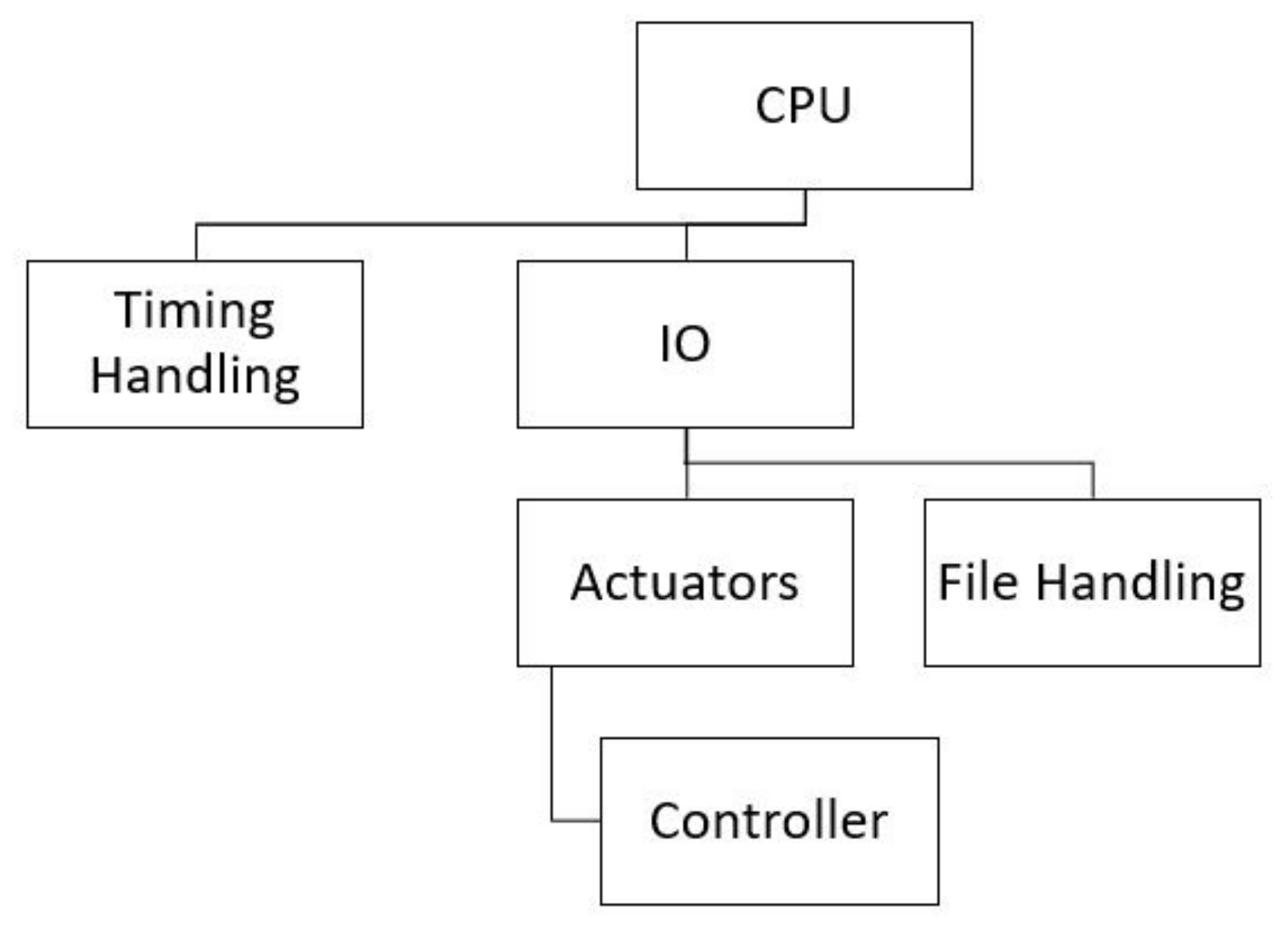
Our new approach simplifies the robot control system, reducing development time significantly. All the parts of the control system can be seen in Figure 2. As is obvious, developing such a control system is much quicker than developing a more typical control system architecture. However, this is just a bare minimum approach. Expanding the control system to support IO, network, etc., still works using offline kinematics calculation.
Simplifying the control system does come at a cost. The biggest drawback of having a control system which uses offline kinematics calculation is that real-time correction of robot poses is not possible.
3. Kinematics
The position and rotational pose of the end effector of serial link robot can be described as a series of transformations where each transformation is from the previous joint to the current joint. The form of a transformation can be seen in Equation (1).
where is the rotation matrix, is a vector which represents the displacement, is the zero vector.
A popular approach to setting up transformation between links is the Denavit-Hartenberg (DH) convention. The DH parameters can be extracted from the robot and the corresponding transformation calculated. The transformation using the DH convention can be done as follows:
where d is the offset between the common normal along the previous , is the angle between the old to the new , about the previous , a is the length of the common normal, and is the angle from old axis to new axis, about the common normal. The -axis is completed with the right hand rule.
Multiplying all the link transformations then gives the total transformation from the base of the robot to the end effector. This is called the forward kinematics, where the joint values are known, and the end effector pose is calculated. The opposite problem, finding the joint values with a given end effector pose, is called the inverse kinematics.
3.1. Inverse Kinematics
There are multiple approaches to calculating the inverse kinematics. One approach for solving the inverse kinematics is by finding a closed form solution, which gives a direct mapping from Cartesian space to the joint space. While the closed-form solution is the most computational effective solution, it may sometimes be difficult, or even impossible, to find. Another approach is by using a numerical technique. Instead of finding a closed-form solution which gives the correct solution after one iteration, a numerical technique converges towards a correct solution after several iteration. In recent years, there has also been an interest in using artificial intelligence, with a bias towards Artificial Neural Networks, for solving the inverse kinematics problem.
For our approach, we are using the numerical technique CLIK to solve the inverse kinematics problem. This is chosen for simplicity and re-configurability, and since speed and computational efficiency is not of primary concern. An overview of the numerical technique can be seen in Figure 3.
The inverse kinematics is solved by taking the Jacobian of the current robot pose, taking the inverse of it, and multiplying it with an vector that represents the error in positioning and rotation and a gain (K). The Jacobian is the mapping between the joint velocities and the corresponding end effector linear and angular velocity. A step towards the desired pose is then achieved. This is repeated until the joint angles that give the desired pose is found. If it does not converge after a number of steps, it is likely that the pose is at a singularity, or outside the work envelope of the robot.
The Jacobian for a series of revolute joints can be found as follows:
where is the axis of rotation for the nth axis (with a zero-index), is the position of the nth joint.
The Jacobian for a series of prismatic joints can be found as follows:
The two equations can be combined to find the Jacobian for a manipulator consisting of both revolute and prismatic joints.
Another benefit of this approach to solving the inverse kinematics is that is it is easy to reconfigure to a new robot, only the transformations between the links needs to be changed. With a closed form solution, all the expressions needs to change when a new manipulator design is to be calculated.
3.2. Trajectory Planning
Another important step for a robotic control system is trajectory planning. Simple point to point motion for the end effector only needs the inverse kinematics solved for the start point and the end point, and the servos can move in whatever order to reach the desired pose. However, when the trajectory of the end effector is of concern, certain steps have to be taken. The most common trajectory between two points is a linear translation accompanied with a simultaneous linear rotation. The Jacobian can be used calculate the joint velocities in order to move the end effector with a constant linear velocity. However, since for a real world application the output to the joint angles has to be discretized, a simpler approach is to calculate the joint angles for a set of points on a line, resulting in approximate linear path.
4. Implementation with a Custom Robot
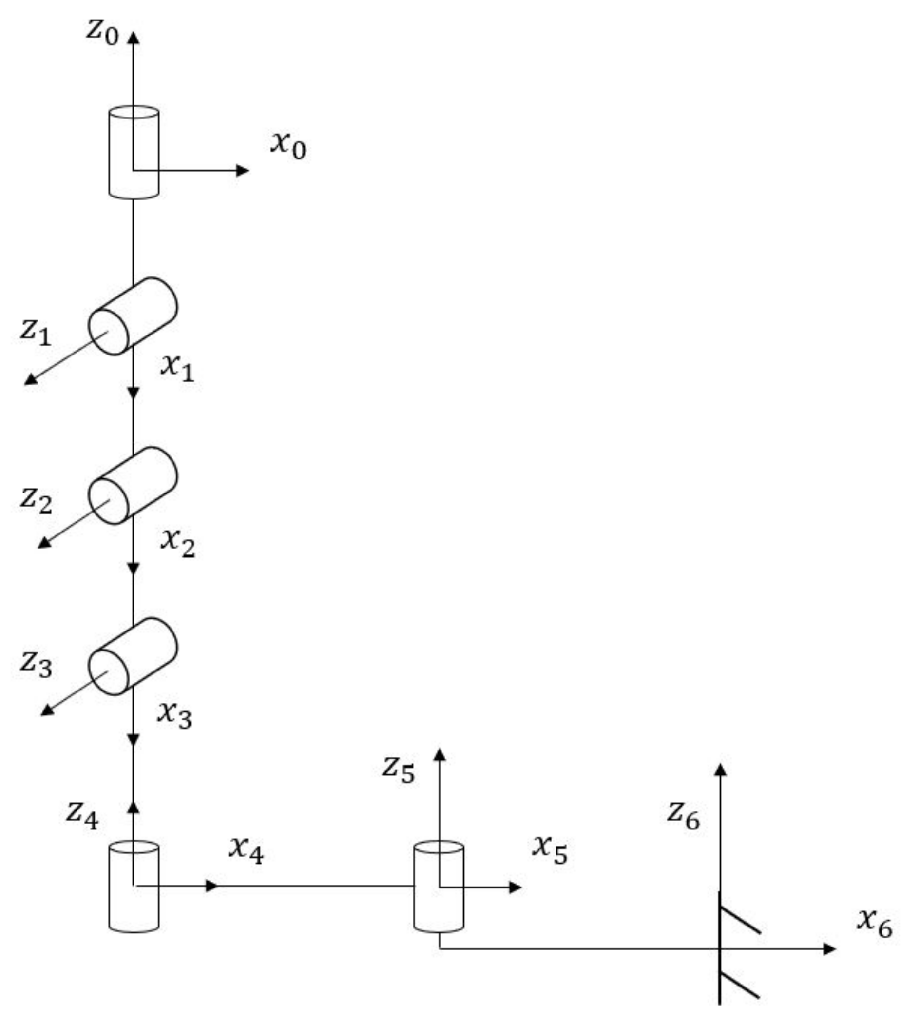
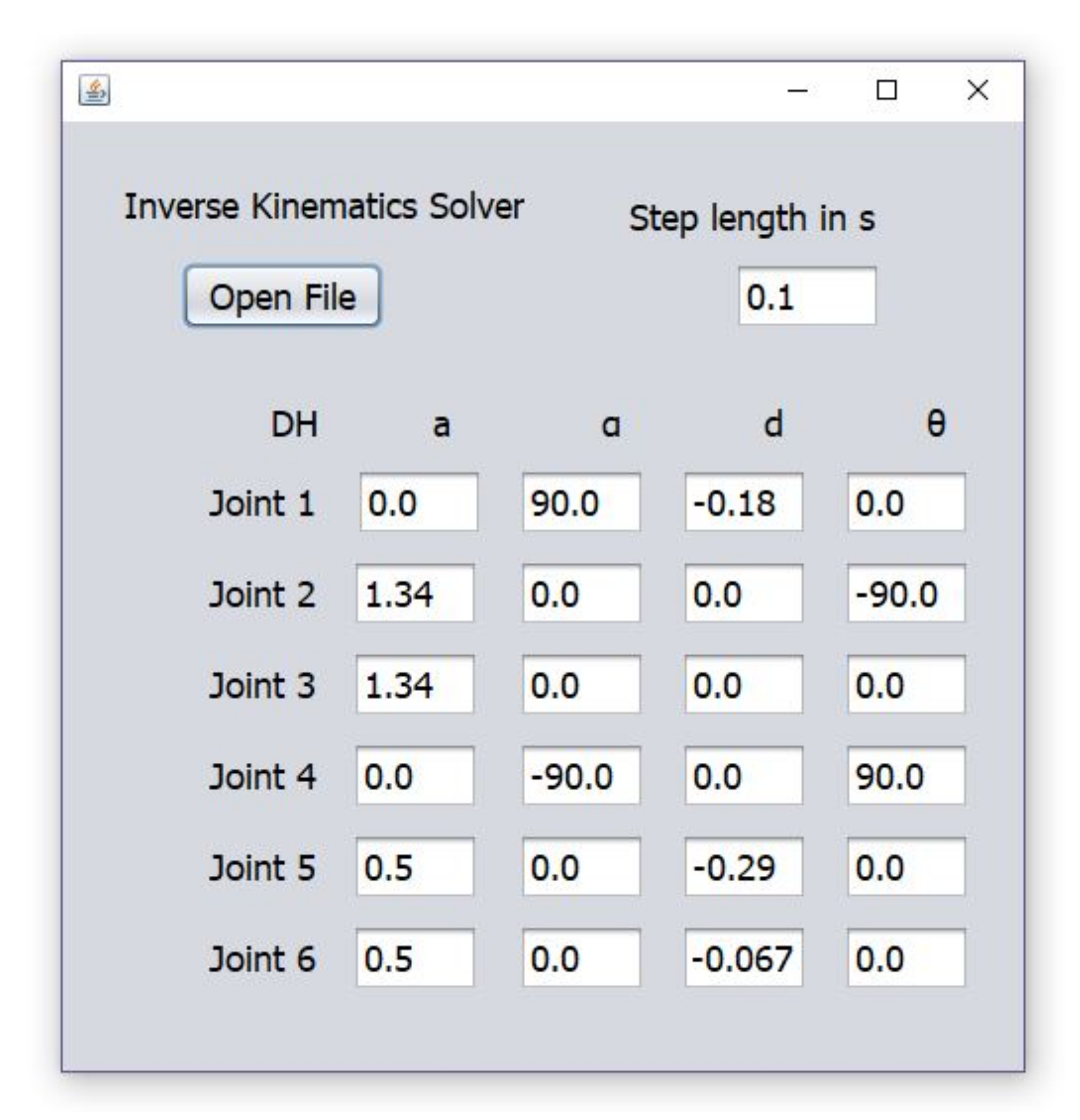
To test the Inverse Kinematics solver, a robot was set up in the DH table, and the inverse kinematics was calculated. A figure of the custom robot can be seen in Figure 4. Due to the nature of the DH convention, joint 4 has to be considered as overlapping with joint 3. For simplicity, this is not taken into account in the figure. The DH table can be seen in Table 1. The graphical user interface (GUI) with the implemented DH table can be seen in Figure 5.
4.1. Format
The format of the input file is as follows:
Motion Type: Either PTP, for Point to Point motion, or LIN, for a linear trajectory from the previous pose to the new pose.
X: The x coordinate of the end effector, with respect to the base frame.
Y: The y coordinate of the end effector, with respect to the base frame.
Z: The z coordinate of the end effector, with respect to the base frame.
Roll: Roll angle of the end effector. Angle, in radians, around the x-axis of the current frame (which is parallel to the x-axis of the base frame).
Pitch: Pitch angle of the end effector. Angle, in radians, around the current y-axis.
Yaw: Yaw angle of the end effector. Angle, in radians, around the current z-axis.
Configuration bit 1: Configuration bit for deciding “elbow up” or “elbow down” in joint 3.
Configuration bit 2: Configuration bit for deciding “elbow to the right” or “elbow to the left” for joint 6. However, this is just for that specific implementation, in reality it is just a check for the joint value at joint 3 and, and if it opposite of what the configuration bit says it should be, change the sign.
Velocity: Velocity of the end effector. For PTP, this is a relative velocity, where 100 is 100% velocity, dictated by the joint that has the furthest to travel. The other joints will move with reduced velocity in order to reach the desired joint angles simultaneously. For LIN, the value is in m/s. The value will dictate how many interpolated points will be generated.
Acceleration: Acceleration of the end effector.
The fields in the input is delimited by a space. An example of an input file can be seen in Table 2.
The format of the output file is the 6 joint values, in radians. The resulting output from the input in Table 2, can be seen in Table 3.
An example of a LIN motion can be seen in the table. The previous motion is added for reference of the start point. The LIN motion is calculated with a step length of 100 ms, beginning at time 0 ms.
4.2. Computation Time
As discussed previously, the computational speed of the inverse kinematics is not of great concern for offline calculation. However, if the inverse calculator is to be implemented in an online application the computational speed is of great concern. For this reason, the computation time for the input set in Table 2 and the resulting output, Table 3, was measured. Since the LIN motion results in several steps with the same step length, and thus the same number of iterations, some of them have been omitted. Bearing in mind that a standard PC has a lot of computational power, it comes as no surprise that even single thread computation of a lot of iterations are completed in a short amount of time. Some computation times can be seen in Table 4. This is done with a gain of 0.2 for position and 0.1 for rotation, on a Intel Core i7 7700 CPU. The initial guess for the joint values for the first iteration is 0.0 for all joints.
5. Optimizing Gain Using GA
5.1. Genetic Algorithm
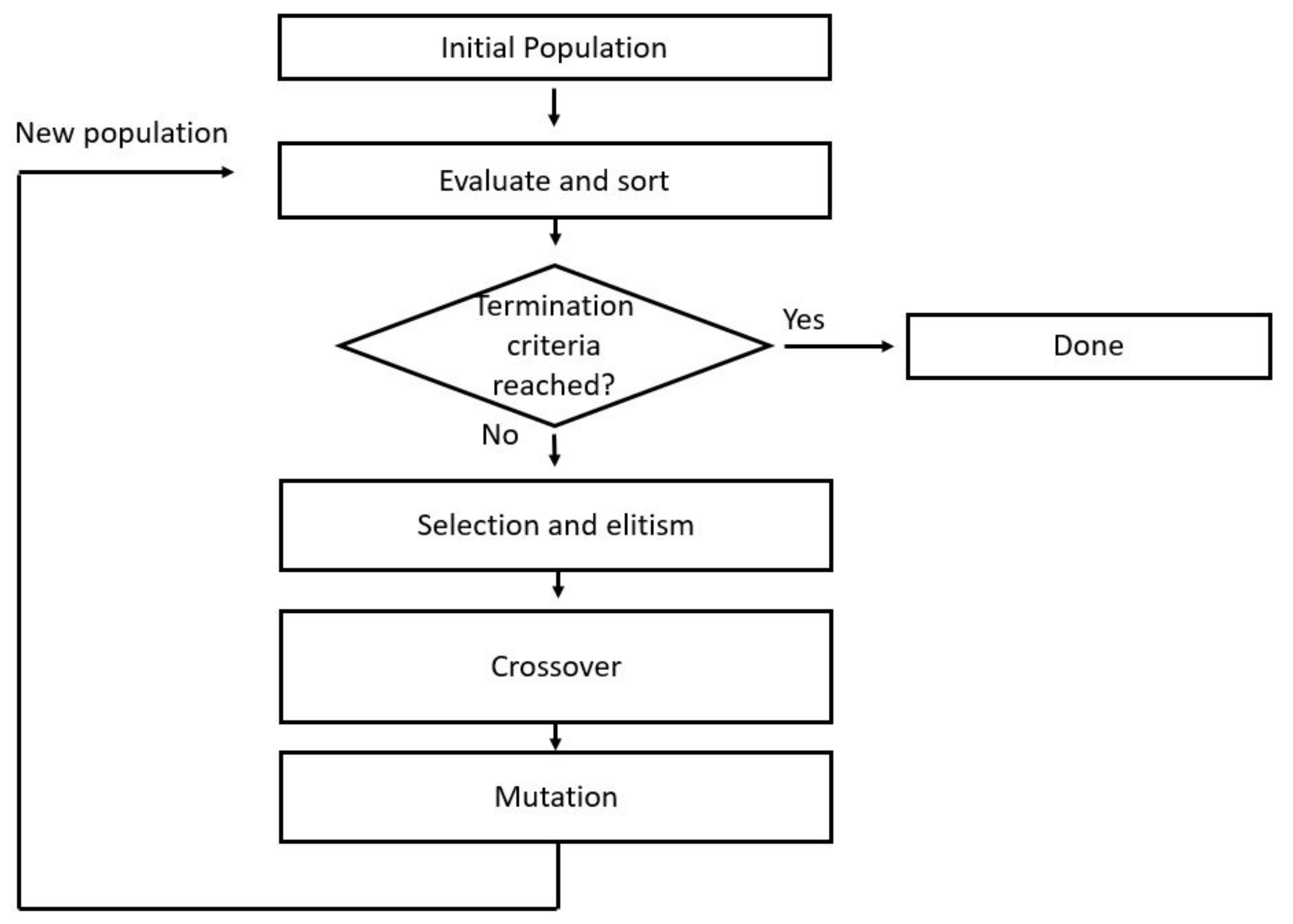
The Genetic Algorithm is a heuristic inspired by the natural selection found in nature that belongs in the larger class Evolutionary Algorithms. Genetic algorithms became popular in the 1970s by the book Adaptation in Natural and Artificial systems by John Holland [36]. A series of candidate solutions with random attributes are initially generated. This is called a population. The individuals of the population are then evaluated with the given cost/fitness function. The population is then evolved into (hopefully) a better population. This evolution process mimics nature, by breeding, mutation and survival of the fittest. A flow chart of the GA can be seen in Figure 6.
5.2. Experimental Setup
The experiment was implemented using the previously discussed CLIK algorithm. The gain was divided into two; gain for the position, and gain for the rotation. The setting for the GA can be seen in Table 5. The manipulator DH table can be seen in Table 1. The Inverse Kinematics loop was set to loop a maximum of 1000 iterations. Either the gain is too high and the loop keeps oscillating, or the gain is too low, and will require too many iterations to converge.
In order to test the candidate solutions, a test set had to be generated. For each joint, a random number between 0 and 1.5 was chosen. A total number of 64 configurations with random numbers on each joint was generated. From each of these joint sets, the forward kinematics for the robot was calculated. When testing the candidate solutions, an initial joint set consisting of random values for each joint was generated. The candidates were evaluated by adding all the iterations necessary to complete the inverse kinematics calculation for all the different manipulator poses. When a candidate solution did not converge, i.e., reached 1000 iterations, a penalty of 1,000,000 was added. In case of a non-converging solution, the rest of the calculations for that solution is aborted. By adding a penalty of 1,000,000, the candidate solution that did not converge could easily be uncovered. The GA was modified to drop the candidate solutions that did not converge, and instead generate new random individuals in the population.
In addition to implementing elitism in the GA, for each elite individual, two new individuals with the same chromosome as the elite individual was generated. A random value between −0.2 and 0.2 were then added to each chromosome of the new individuals, expanding the search around the elite individuals.
5.3. Result
The result of the GA can be seen in Table 6. It is interesting to note the disparity of the candidate solutions.
5.4. Retesting the Calculation from Section 4.2
Finally, the new gain constants from the best chromosome were tested in the IKS for the same data set as used in Section 4.2. The results can be seen in Table 7. It is interesting to see that in most cases, the number of iterations has dropped significantly, but the computation time is not linearly dependent on the number of iterations. The result from calculating the inverse kinematics with the new gain can be seen in Table 8. It is interesting to see that the solution is not the same as with the gain used to get Table 3.
6. Discussion and Conclusions
Separating the inverse kinematics calculations from the robot control system, and keeping the number of tasks for the robot control system to a minimum can reduce the time to develop such a system. Realizing the Inverse Kinematics Solver in Java was a straight forward task, and may enable others to build robot control systems quicker.
At this stage, the Inverse Kinematics Solver is limited to six revolute joints, with the DH table set within the program. A future version should have coverage for a varying number of joints and prismatic joints, with the possibility to set it all up from the GUI. In addition, the rotations are done by Euler angles. This may result in singularity problems, and using quaternions might be a better option. The IKS could also be expanded to include trajectory generation for circular motions.
Optimizing the gain of the IKS with GA gave, as can be seen in the results, a much quicker convergence than randomly selecting some gain. However, the author could not find any other research which focused on optimizing the gain of the CLIK with respect to computational speed, so doing a quantitative comparison to other approaches was not possible. This might be due to the fact that if the desired robot pose is far from singularity, and the initial guess is quite good, the gain for the feedback can be as high as 1, which is the same as not multiplying the feedback by any factor.
In addition, the CLIK in this current implementation does not have any mechanism for handling solutions that are singular or very close to singular. Singularities will result in an inverse Jacobian where one or more of the element will have a high value, increasing the chance for the CLIK to oscillate. Implementing a mechanism for handling this problem, for instance Damped Least Squares, might have a high influence of the optimal gain of the loop, possibly resulting in even quicker convergence. However, with the current lack of singularity handling, the GA finds an optimal solution which does not oscillate, even at singular poses.
Acknowledgments
This research was funded by the Research Council of Norway, grant no. 245613/O30.
Conflicts of Interest
The authors declare no conflict of interest.
References
- Lyons, D.M.; Arbib, M.A. A formal model of computation for sensory-based robotics. IEEE Trans. Robot. Autom. 1989, 5, 280–293. [Google Scholar] [CrossRef]
- Zielinski, C. A quasi-formal approach to structuring multi-robot system controllers. In Proceedings of the 2001 the Second International Workshop on Robot Motion and Control, Bukowy Dworek, Poland, 18–20 October 2001; pp. 121–128. [Google Scholar]
- Pan, Z.; Polden, J.; Larkin, N.; Duin, S.V.; Norrish, J. Recent Progress on Programming Methods for Industrial Robots. In Proceedings of the ISR 2010 (41st International Symposium on Robotics) and ROBOTIK 2010 (6th German Conference on Robotics), Munich, Germany, 7–9 June 2010; pp. 1–8. [Google Scholar]
- Thomessen, T.; Sannæs, P.K.; Lien, T.K. Intuitive Robot Programming. In Proceedings of the 35th International Symposium on Robotics, Paris-Nord Villepinte, France, 23–26 March 2004. [Google Scholar]
- International Federation of Robotics. World Robotics; International Federation of Robotics: Frankfurt, Germany, 2013. [Google Scholar]
- Zieliński, C.; Stefańczyk, M.; Kornuta, T.; Figat, M.; Dudek, W.; Szynkiewicz, W.; Kasprzak, W.; Figat, J.; Szlenk, M.; Winiarski, T.; et al. Variable structure robot control systems: The RAPP approach. Robot. Auton. Syst. 2017, 94, 226–244. [Google Scholar] [CrossRef]
- El-Sherbiny, A.; Elhosseini, M.A.; Haikal, A.Y. A comparative study of soft computing methods to solve inverse kinematics problem. Ain Shams Eng. J. 2017, in press. [Google Scholar] [CrossRef]
- McEvoy, M.A.; Correll, N. Distributed Inverse Kinematics for Shape-changing Robotic Materials. Procedia Technol. 2016, 26, 4–11. [Google Scholar] [CrossRef]
- Kucuk, S.; Bingul, Z. Inverse kinematics solutions for industrial robot manipulators with offset wrists. Appl. Math. Model. 2014, 38, 1983–1999. [Google Scholar] [CrossRef]
- Burrell, T.; Montazeri, A.; Monk, S.; Taylor, C.J. Feedback Control—Based Inverse Kinematics Solvers for a Nuclear Decommissioning Robot. IFAC-PapersOnLine 2016, 49, 177–184. [Google Scholar] [CrossRef]
- Toshani, H.; Farrokhi, M. Real-time inverse kinematics of redundant manipulators using neural networks and quadratic programming: A Lyapunov-based approach. Robot. Auton. Syst. 2014, 62, 766–781. [Google Scholar] [CrossRef]
- Duka, A.V. Neural Network based Inverse Kinematics Solution for Trajectory Tracking of a Robotic Arm. Procedia Technol. 2014, 12, 20–27. [Google Scholar] [CrossRef]
- Aristidou, A.; Lasenby, J. Inverse Kinematics: A Review of Existing Techniques and Introduction of a New Fast Iterative Solver; Department of Engineering, University of Cambridge: Cambridge, UK, 2009. [Google Scholar]
- Benhabib, B.; Goldenberg, A.A.; Fenton, R.G. A Solution to the Inverse Kinematics of Redundant Manipulators. In Proceedings of the 1985 American Control Conference, Boston, MA, USA, 19–21 June 1985; pp. 368–374. [Google Scholar]
- Goldenberg, A.; Benhabib, B.; Fenton, R. A complete generalized solution to the inverse kinematics of robots. IEEE J. Robot. Autom. 1985, 1, 14–20. [Google Scholar] [CrossRef]
- Sciavicco, L.; Siciliano, B. Coordinate Transformation: A Solution Algorithm for One Class of Robots. IEEE Trans. Syst. Man Cybern. 1986, 16, 550–559. [Google Scholar] [CrossRef]
- Das, H.; Slotine, J.E.; Sheridan, T.B. Inverse kinematic algorithms for redundant systems. In Proceedings of the 1988 IEEE International Conference on Robotics and Automation, Philadelphia, PA, USA, 24–29 April 1988; Volume 1, pp. 43–48. [Google Scholar]
- Falco, P.; Natale, C. On the Stability of Closed-Loop Inverse Kinematics Algorithms for Redundant Robots. IEEE Trans. Robot. 2011, 27, 780–784. [Google Scholar] [CrossRef]
- Bjerkeng, M.; Falco, P.; Natale, C.; Pettersen, K.Y. Stability Analysis of a Hierarchical Architecture for Discrete-Time Sensor-Based Control of Robotic Systems. IEEE Trans. Robot. 2014, 30, 745–753. [Google Scholar] [CrossRef]
- Vito, D.D.; Natale, C.; Antonelli, G. A Comparison of Damped Least Squares Algorithms for Inverse Kinematics of Robot Manipulators. IFAC-PapersOnLine 2017, 50, 6869–6874. [Google Scholar]
- Kumar, S.L. State of the Art-Intense Review on Artificial Intelligence Systems Application in Process Planning and Manufacturing. Eng. Appl. Artif. Intell. 2017, 65, 294–329. [Google Scholar] [CrossRef]
- Zhong, Y.; Lin, J.; Wang, L.; Zhang, H. Hybrid discrete artificial bee colony algorithm with threshold acceptance criterion for traveling salesman problem. Inf. Sci. 2017, 421, 70–84. [Google Scholar] [CrossRef]
- Nasiri, S.; Khosravani, M.R.; Weinberg, K. Fracture mechanics and mechanical fault detection by artificial intelligence methods: A review. Eng. Fail. Anal. 2017, 81, 270–293. [Google Scholar] [CrossRef]
- Kouziokas, G.N. The application of artificial intelligence in public administration for forecasting high crime risk transportation areas in urban environment. Transp. Res. Procedia 2017, 24, 467–473. [Google Scholar] [CrossRef]
- Dande, P.; Samant, P. Acquaintance to Artificial Neural Networks and use of artificial intelligence as a diagnostic tool for tuberculosis: A review. Tuberculosis 2018, 108, 1–9. [Google Scholar] [CrossRef]
- Li, J.; Zhang, L.; ShangGuan, C.; Kise, H. A GA-based heuristic algorithm for non-permutation two-machine robotic flow-shop scheduling problem of minimizing total weighted completion time. In Proceedings of the 2010 IEEE International Conference on Industrial Engineering and Engineering Management, Macao, China, 7–10 December 2010; pp. 1281–1285. [Google Scholar]
- Sharma, R.; Rana, K.P.S.; Kumar, V. Statistical analysis of GA based PID controller optimization for robotic manipulator. In Proceedings of the 2014 International Conference on Issues and Challenges in Intelligent Computing Techniques (ICICT), Ghaziabad, India, 7–8 February 2014; pp. 713–718. [Google Scholar]
- Gu, D.; Hu, H.; Reynolds, J.; Tsang, E. GA-based learning in behaviour based robotics. In Proceedings of the 2003 IEEE International Symposium on Computational Intelligence in Robotics and Automation. Computational Intelligence in Robotics and Automation for the New Millennium (Cat. No.03EX694), Kobe, Japan, 16–20 July 2003; Volume 3, pp. 1521–1526. [Google Scholar]
- Fukuda, T.; Shimojima, K. Fusion of fuzzy, NN, GA to the intelligent robotics. In Proceedings of the 1995 IEEE International Conference on Systems, Man and Cybernetics. Intelligent Systems for the 21st Century, Vancouver, BC, Canada, 22–25 October 1995; Volume 3, pp. 2892–2897. [Google Scholar]
- McCrea, A.; Navon, R. Application of GA in optimal robot selection for bridge restoration. Autom. Constr. 2004, 13, 803–819. [Google Scholar] [CrossRef]
- Kumar, A.; Kumar, V. Hybridized ABC-GA optimized fractional order fuzzy pre-compensated FOPID control design for 2-DOF robot manipulator. AEU—Int. J. Electron. Commun. 2017, 79, 219–233. [Google Scholar] [CrossRef]
- Köker, R. A genetic algorithm approach to a neural-network-based inverse kinematics solution of robotic manipulators based on error minimization. Inf. Sci. 2013, 222, 528–543, (Including Special Section on New Trends in Ambient Intelligence and Bio-inspired Systems). [Google Scholar] [CrossRef]
- Caponetto, R.; Fortuna, L.; Fazzino, S.; Xibilia, M.G. Chaotic sequences to improve the performance of evolutionary algorithms. IEEE Trans. Evolut. Comput. 2003, 7, 289–304. [Google Scholar] [CrossRef]
- Mozafar, M.R.; Moradi, M.H.; Amini, M.H. A simultaneous approach for optimal allocation of renewable energy sources and electric vehicle charging stations in smart grids based on improved GA-PSO algorithm. Sustain. Cities Soc. 2017, 32, 627–637. [Google Scholar] [CrossRef]
- Zhou, H.; Song, M.; Pedrycz, W. A Comparative Study of Improved GA and PSO in Solving Multiple Traveling Salesmen Problem. Appl. Soft Comput. 2017, 64, 564–580. [Google Scholar] [CrossRef]
- Holland, J.H. Adaptation in Natural and Artificial Systems: An Introductory Analysis with Applications to Biology, Control and Artificial Intelligence; MIT Press: Cambridge, MA, USA, 1992. [Google Scholar]
Figure 1.
Overview of a typical robot control system architecture.
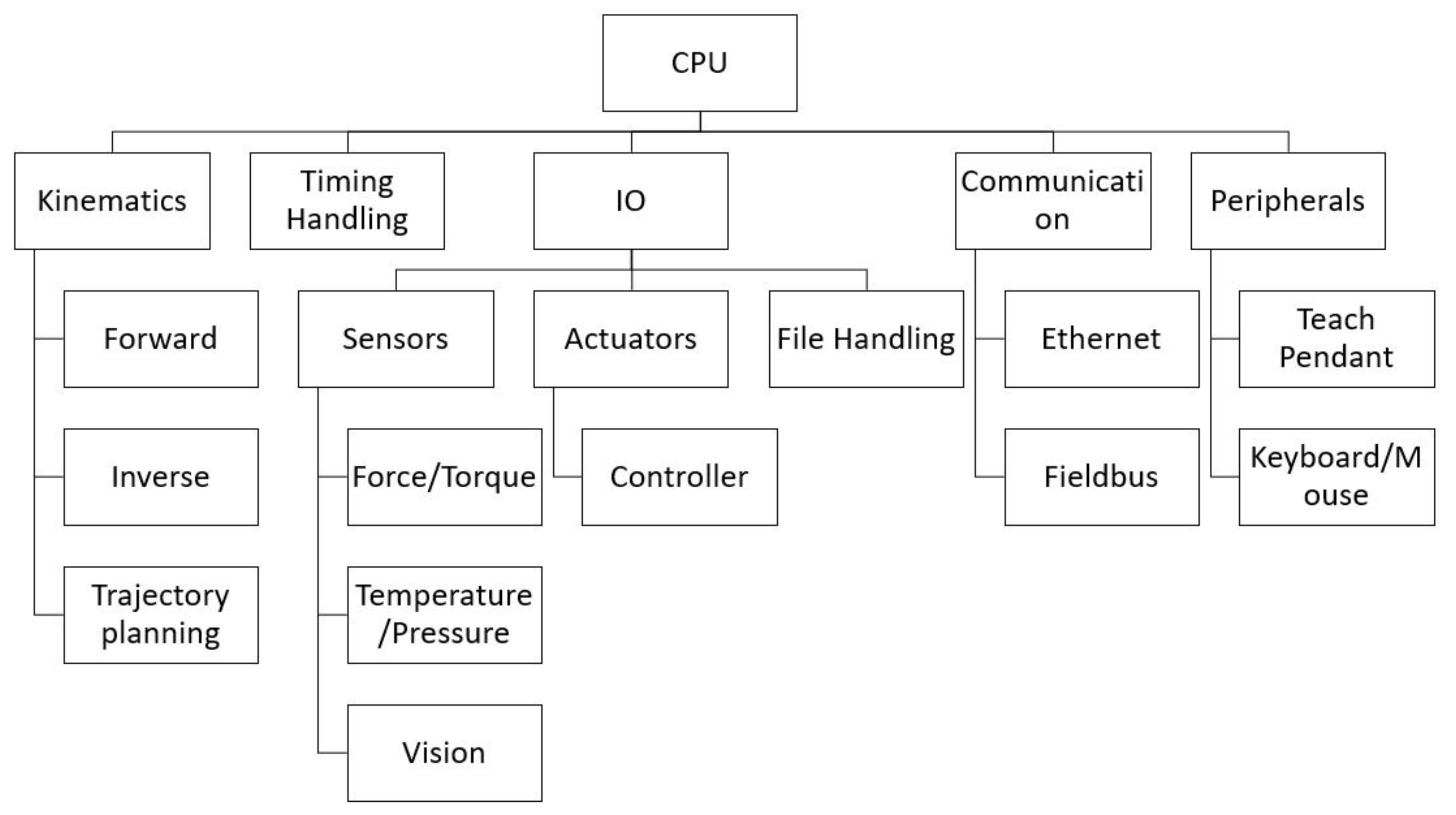
Figure 2.
Overview of the simplified robot control system.

Figure 3.
The numerical loop to calculate the inverse kinematics.
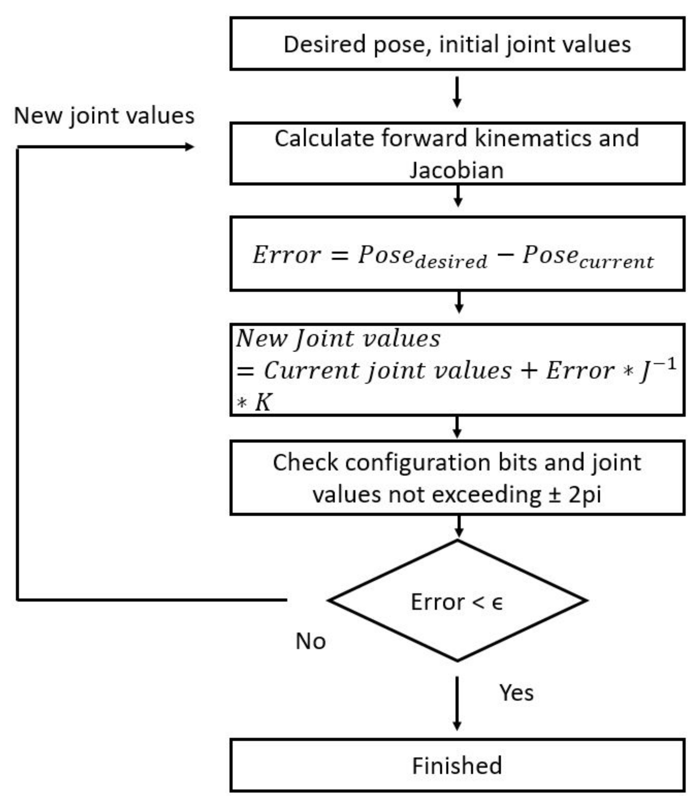
Figure 4.
The robot in the home position. Not drawn to scale.

Figure 5.
The GUI of the Inverse Kinematics Solver (IKS).

Figure 6.
Flow chart of the GA process.

Table 1.
Denavit-Hartenberg (DH) parameters of the custom robot.
| 1 | −180 | 0 | 0 | 90 |
| 2 | 0 | −90 | 1340 | 0 |
| 3 | 0 | 0 | 1340 | 0 |
| 4 | 0 | 90 | 0 | −90 |
| 5 | −290 | 0 | 500 | 0 |
| 6 | −67 | 0 | 500 | 0 |
Table 2.
Input file.
| Motion Type | X | Y | Z | R | P | Y | Config 1 | Config 2 | Vel. | Acc. |
|---|---|---|---|---|---|---|---|---|---|---|
| PTP | 0.500 | 0.010 | −2.700 | 0.0 | 0.0 | 0.0 | 1 | 1 | 50 | 50 |
| PTP | 0.500 | 0.010 | −2.800 | 0.0 | 0.0 | 0.0 | 1 | 1 | 25 | 25 |
| PTP | 0.500 | 0.010 | −2.900 | 0.0 | 0.0 | 0.0 | 0 | 0 | 50 | 50 |
| PTP | 0.500 | 0.010 | −2.800 | 0.0 | 0.0 | 0.0 | 1 | 1 | 50 | 50 |
| LIN | 0.500 | 0.010 | −2.700 | 0.0 | 0.0 | 0.0 | 1 | 1 | 0.05 | 50 |
Table 3.
Calculated output.
| Joint 1 | Joint 2 | Joint 3 | Joint 4 | Joint 5 | Joint 6 |
|---|---|---|---|---|---|
| −0.2834 | −0.8226 | 1.1884 | −0.3658 | 0.0192 | 0.2642 |
| −0.2832 | −0.7446 | 1.0519 | −0.3073 | 0.0192 | 0.2639 |
| 0.0237 | 0.2399 | −0.8965 | 0.6566 | 0.02 | −0.0437 |
| −0.2814 | −0.7443 | 1.0514 | −0.3071 | 0.0192 | 0.2621 |
| −0.2814 | −0.7443 | 1.0514 | −0.3071 | 0.0192 | 0.2621 |
| −0.2814 | −0.7483 | 1.0584 | −0.3102 | 0.0192 | 0.2622 |
| −0.2814 | −0.7525 | 1.066 | −0.3135 | 0.0192 | 0.2622 |
| −0.2814 | −0.7568 | 1.0735 | −0.3167 | 0.0192 | 0.2622 |
| −0.2814 | −0.761 | 1.081 | −0.32 | 0.0192 | 0.2622 |
| −0.2814 | −0.7652 | 1.0884 | −0.3232 | 0.0192 | 0.2622 |
| −0.2815 | −0.7694 | 1.0958 | −0.3263 | 0.0192 | 0.2622 |
| −0.2815 | −0.7736 | 1.1031 | −0.3295 | 0.0192 | 0.2623 |
| −0.2815 | −0.7778 | 1.1104 | −0.3326 | 0.0192 | 0.2623 |
| −0.2815 | −0.7819 | 1.1176 | −0.3358 | 0.0192 | 0.2623 |
| −0.2815 | −0.786 | 1.1248 | −0.3388 | 0.0192 | 0.2623 |
| −0.2815 | −0.7901 | 1.132 | −0.3419 | 0.0192 | 0.2623 |
| −0.2815 | −0.7942 | 1.1391 | −0.345 | 0.0192 | 0.2623 |
| −0.2816 | −0.7982 | 1.1462 | −0.348 | 0.0192 | 0.2623 |
| −0.2816 | −0.8023 | 1.1533 | −0.351 | 0.0192 | 0.2624 |
| −0.2816 | −0.8063 | 1.1603 | −0.3539 | 0.0192 | 0.2624 |
| −0.2816 | −0.8103 | 1.1672 | −0.3569 | 0.0192 | 0.2624 |
| −0.2816 | −0.8143 | 1.1741 | −0.3598 | 0.0192 | 0.2624 |
| −0.2816 | −0.8183 | 1.181 | −0.3627 | 0.0192 | 0.2624 |
| −0.2816 | −0.8223 | 1.1879 | −0.3656 | 0.0192 | 0.2624 |
Table 4.
Iterations needed and the computation time for the different poses in Table 2.
Table 4.
Iterations needed and the computation time for the different poses in Table 2.
| Line Nr | Nr of Iterations | Time to Complete Calculation () |
|---|---|---|
| 1 | 546 | 68,135 |
| 2 | 25 | 1222 |
| 3 | 113 | 6487 |
| 4 | 270 | 8870 |
| 5 | 1 | 144 |
| 6 | 12 | 606 |
| 7 | 12 | 447 |
| 8 | 12 | 399 |
| 24 | 12 | 484 |
Table 5.
Parameters of the GA.
| Population size | 100 |
| Nr of Elite | 8 |
| Nr of Near Searches pr Elite | 2 |
| Mutation Rate | 0.5 |
| Evolution iterations | 5 |
Table 6.
The best individuals in the GA.
| Solution Placing | Number of Iterations | Gene 1 | Gene 2 |
|---|---|---|---|
| 1 | 1117 | 0.6229 | 0.8046 |
| 2 | 1216 | 0.9566 | 0.9642 |
| 3 | 1223 | 0.8731 | 1.1492 |
| 4 | 1259 | 0.7766 | 0.9969 |
Table 7.
Iterations needed and the computation time for the different poses in Table 2 with gain from the best chromosome.
Table 7.
Iterations needed and the computation time for the different poses in Table 2 with gain from the best chromosome.
| Line Nr | Nr of Iterations | Time to Complete Calculation (s) |
|---|---|---|
| 1 | 47 | 15,075 |
| 2 | 7 | 1132 |
| 3 | 11 | 1518 |
| 4 | 31 | 4208 |
| 5 | 7 | 1035 |
| 6 | 9 | 606 |
| 7 | 4 | 516 |
| 8 | 4 | 487 |
| 24 | 4 | 567 |
Table 8.
Calculated output with optimized gain.
| Joint 1 | Joint 2 | Joint 3 | Joint 4 | Joint 5 | Joint 6 |
|---|---|---|---|---|---|
| −0.0199 | −0.8218 | 1.1892 | −0.3674 | −0.0199 | 0 |
| −0.02 | −0.7437 | 1.0524 | −0.3087 | 0.0199 | 0.0001 |
| −0.0108 | 0.2397 | −0.8964 | 0.6567 | 0.02 | −0.0092 |
| −0.0199 | −0.7436 | 1.0522 | −0.3086 | −0.0199 | 0 |
| −0.0199 | −0.7436 | 1.0522 | −0.3086 | 0.0199 | 0 |
| −0.02 | −0.7479 | 1.0598 | −0.3119 | 0.0199 | 0.0001 |
| −0.02 | −0.7521 | 1.0672 | −0.3151 | 0.02 | 0 |
| −0.02 | −0.7563 | 1.0747 | −0.3184 | 0.02 | 0 |
| −0.0201 | −0.7606 | 1.0822 | −0.3216 | 0.02 | 0.0001 |
| −0.0201 | −0.7648 | 1.0896 | −0.3248 | 0.02 | 0.0001 |
| −0.0201 | −0.769 | 1.097 | −0.328 | 0.02 | 0.0001 |
| −0.0201 | −0.7731 | 1.1043 | −0.3312 | 0.02 | 0.0001 |
| −0.0201 | −0.7773 | 1.1116 | −0.3343 | 0.02 | 0.0001 |
| −0.0201 | −0.7814 | 1.1188 | −0.3374 | 0.02 | 0.0001 |
| −0.0201 | −0.7855 | 1.126 | −0.3405 | 0.02 | 0.0001 |
| −0.0202 | −0.7896 | 1.1332 | −0.3436 | 0.02 | 0.0002 |
| −0.0202 | −0.7937 | 1.1403 | −0.3466 | 0.02 | 0.0002 |
| −0.0202 | −0.7977 | 1.1474 | −0.3496 | 0.02 | 0.0002 |
| −0.0202 | −0.8018 | 1.1544 | −0.3526 | 0.02 | 0.0002 |
| −0.0202 | −0.8058 | 1.1614 | −0.3556 | 0.02 | 0.0002 |
| −0.0202 | −0.8098 | 1.1684 | −0.3586 | 0.02 | 0.0002 |
| −0.0202 | −0.8138 | 1.1753 | −0.3615 | 0.02 | 0.0002 |
| −0.0203 | −0.8178 | 1.1822 | −0.3644 | 0.02 | 0.0003 |
| −0.0203 | −0.8217 | 1.189 | −0.3673 | 0.02 | 0.0003 |
© 2018 by the author. Licensee MDPI, Basel, Switzerland. This article is an open access article distributed under the terms and conditions of the Creative Commons Attribution (CC BY) license (http://creativecommons.org/licenses/by/4.0/).
Share and Cite
MDPI and ACS Style
Bjoerlykhaug, E.D. A Closed Loop Inverse Kinematics Solver Intended for Offline Calculation Optimized with GA. Robotics 2018, 7, 7. https://doi.org/10.3390/robotics7010007
AMA Style
Bjoerlykhaug ED. A Closed Loop Inverse Kinematics Solver Intended for Offline Calculation Optimized with GA. Robotics. 2018; 7(1):7. https://doi.org/10.3390/robotics7010007
Chicago/Turabian StyleBjoerlykhaug, Emil Dale. 2018. "A Closed Loop Inverse Kinematics Solver Intended for Offline Calculation Optimized with GA" Robotics 7, no. 1: 7. https://doi.org/10.3390/robotics7010007
Note that from the first issue of 2016, this journal uses article numbers instead of page numbers. See further details here.