Close Range Tracking of an Uncooperative Target in a Sequence of Photonic Mixer Device (PMD) Images ^†

Abstract

This paper presents a pose estimation routine for tracking attitude and position of an uncooperative tumbling spacecraft during close range rendezvous. The key innovation is the usage of a Photonic Mixer Device (PMD) sensor for the first time during space proximity for tracking the pose of the uncooperative target. This sensor requires lower power consumption and higher resolution if compared with existing flash Light Identification Detection and Ranging (LiDAR) sensors. In addition, the PMD sensor provides two different measurements at the same time: depth information (point cloud) and amplitude of the reflected signal, which generates a grayscale image. In this paper, a hybrid model-based navigation technique that employs both measurements is proposed. The principal pose estimation technique is the iterative closed point algorithm with reverse calibration, which relies on the depth image. The second technique is an image processing pipeline that generates a set of 2D-to-3D feature correspondences between amplitude image and spacecraft model followed by the Efficient Perspective-n-Points (EPnP) algorithm for pose estimation. In this way, we gain a redundant estimation of the target’s current state in real-time without hardware redundancy. The proposed navigation methodology is tested in the German Aerospace Center (DLR)’s European Proximity Operations Simulator. The hybrid navigation technique shows the capability to ensure robust pose estimation of an uncooperative tumbling target under severe illumination conditions. In fact, the EPnP-based technique allows to overcome the limitations of the primary technique when harsh illumination conditions arise.

1. Introduction

Space rendezvous is a key operation required in all the missions involving more than one spacecraft [1]. Considering the problem of space debris removal and future On-Orbit Servicing (OOS) missions, the autonomous close-range approach of a controlled chaser spacecraft towards a target spacecraft is a key-enabling phase in both activities. In order to autonomously navigate to the target, the chaser spacecraft must estimate the pose (i.e., position and orientation) of the target spacecraft regularly during the maneuver.

The autonomous navigation is not only an important action in space applications, but also a key activity for the mobile robots in urban, pedestrian and industrial environments. These robots can perform various tasks with high precision in most severe environments, where the human is not able to complete the required work [2]. The main challenge in the autonomous navigation for the mobile robots is simultaneously map the environment and, moreover, keep track of its pose and location [3]. For this purpose, in the last decay, many distinctive visual navigation techniques using various visual sensors for the map building and robot localization [4,5,6] have been developed and tested.

Concerning space activities and especially the topic on which we are concentrating in this article, Autonomous Rendezvous and Docking (RvD), several autonomous navigation techniques that employ visual-based sensors for motion tracking were applied and tested during real space missions. Examples of such missions are the ETS-VII experiment [7], Orbital Express [8], RvD of the Automated Transfer Vehicle (ATV) to the International Space Station and the Hubble Space Telescope (HST) Servicing Mission 4 (SM4) [9]. In these missions the target spacecraft was always cooperative, since its attitude was stabilized, it communicated its state to the chaser and it was equipped with dedicated visual markers for relative pose estimation.

The difference between the aforementioned in-orbit rendezvous and the close-range approach in future OOS and debris removal missions is the uncooperativeness of the target spacecraft as it is not equipped with dedicated visual markers for distance and attitude estimation and it may tumble around the principal axes. For this reason, new technologies must be developed for the real-time estimation of the pose of the uncooperative target, which represents the key challenge during the autonomous close-range approach. Due to the lack of visual markers, the general approach for uncooperative pose estimation is to extract the most important patterns of the target’s body from the sensor measurements and fit the known shape of the target with the detected features [10]. In general, extracting meaningful features and computing the pose in real time is a challenging task since the detected pattern may vary frame by frame due to the tumbling motion of the target. Moreover, the task is further complicated by the harsh illumination conditions that may occur during the maneuver. By harsh illumination condition we assume excessive levels of sunlight, which oversaturate and distort some pixels of the images. In fact, strong direct sunlight can be reflected by the satellite’s high reflective surfaces covered with Multi-Layer Insulation (MLI) and saturate the sensor’s pixels. Also in this case, unfavorable illumination conditions may arise suddenly due to the uncontrolled motion of the target spacecraft. These high reflections on the target’s surface cause saturation of the sensor pixels, which generate corrupted measurements. On the contrary, complete darkness occurs regularly during each orbit. This situation requires the usage of infrared sensors such as the Light Detection And Ranging (LiDAR) sensor.

Different types of visual sensors have been considered and tested for the close range pose estimation of an uncooperative target spacecraft, viz. LiDAR [11], monocular camera [12,13,14], stereo camera [15,16] and also time-of-flight sensors based on Photonic Mixer Device (PMD) technology [17,18]. LiDAR sensors have high requirements in terms of mass and power, but ensure robustness in any illumination condition as they employ reflected infrared (IR) signals. However, this signal can be reflected multiple times on the target’s surfaces in some particular attitude configurations and thus generate incorrect features in the acquired point cloud [8]. Furthermore, the resolution of the depth measurements must be gradually reduced during the approach to ensure rapid pose estimation in proximity of the target [19]. On the contrary, monocular pose estimation guarantees rapid estimation of the target pose under low mass and power requirements. This approach is robust to reflected features on the target’s surface, but suffers from the harsh illumination conditions of the space environment. With respect to the aforementioned technologies, cameras based on PMD technologies have important advantages, such as the lower mass and power requirements with respect to LiDARs and the capability to provide both depth measurements and 2D images in low-resolution obtained from the reflected signal [17,20]. Due to these advantages, new technologies for uncooperative pose estimation based on PMD measurements have been developed and tested recently. Tzschichholz [18] demonstrated the capability of the PMD sensor to provide raster depth images at a high rate with partly depth data loss when working under strong illumination. In most cases, the real-time pose estimation of the target spacecraft produced accurate results.

In this paper we further investigate the application of the PMD sensor to uncooperative pose estimation and tracking during close-range space rendezvous approaches. We propose a novel navigation technique capable to estimate, even under harsh illumination conditions and with a (partly) depth data loss, the six degrees-of-freedom (DoF) relative pose of the target spacecraft during the close rendezvous phase from 10 to 1 m using the measurement from the PMD sensor. The key feature of the proposed architecture is its hybrid nature, meaning that it employs two different model-based pose estimation techniques to ensure robustness to any illumination condition. The first method estimates the pose of the target spacecraft from the depth measurements using the Iterative Closest Point algorithm (ICP) with a reverse calibration technique. The second method consists of an image processing procedure that extracts low-level features of the target spacecraft from the 2D amplitude images and estimates the current target pose by fitting the projection of the known 3D model on the detected features.

The main contribution of this research is the combination of two different pose estimation techniques for redundant real-time estimation of the target’s state vector without hardware redundancy. To do this, the back-up amplitude images for pose estimation is employed in case of failure of the ICP-based pose estimation with depth images, which is used as primary approach. This ensures applicability and robustness to any illumination condition during the maneuver.

The proposed navigation system was tested in the European Proximity Operations Simulator (EPOS 2.0) [21] at the German Aerospace Center (DLR), which allows real-time simulation of close range proximity operations under realistic space illumination conditions. We tested each designed algorithm for estimation of the relative position and attitude of the satellite mockup in order to compare robustness and accuracy and to identify cases of appliance for each of them.

The paper is organized as follows: Section 2 provides the pose estimation problem of an uncooperative target spacecraft during proximity operations and describes the PMD sensor in detail. Section 3 illustrates the navigation algorithms. Section 4 provides results and analyses of the experimental campaign carried out at EPOS. Finally, Section 5 concludes the paper.

2. Vision Based Navigation During Proximity Operations

2.1. Problem Statement

During close-range proximity operations for OOS and space debris removal missions, the chaser spacecraft performs inspection, rendezvous and docking to an uncooperative target spacecraft. As depicted in Figure 1, the navigation sensor of the chaser spacecraft for close-range rendezvous is a PMD camera (see Section 2.2.1 for sensor specifications) that acquires depth and amplitude images of the target vehicle during the maneuver. The goal of the pose estimation is to determine the relative position vector ${\mathit{t}}^{\mathrm{B}}$ and relative orientation, i.e., attitude, of the target principal frame B with respect to the PMD camera coordinate frame C. Notably in Figure 1a, the attitude of the target spacecraft principal frame B with respect to the camera frame C is represented by the rotation matrix ${\mathit{R}}_{\mathrm{BC}}$.

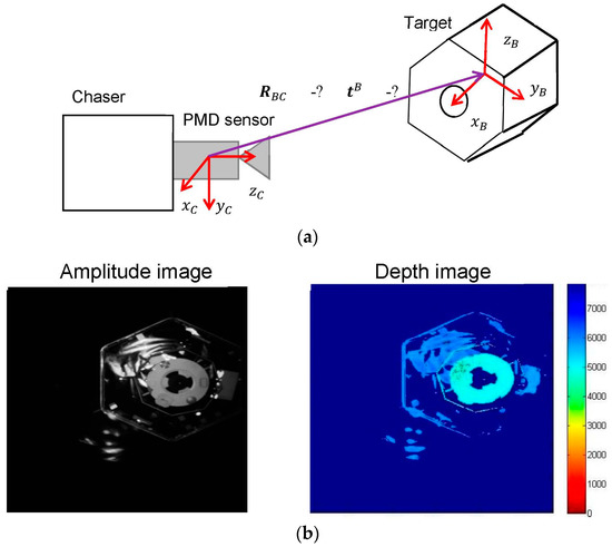
Figure 1. (a) Geometry of the target and the chaser with attached Photonic Mixer Device (PMD) sensor. (b) Example of depth and amplitude images from PMD sensor.

Figure 1b shows an example of amplitude and depth images acquired by the PMD sensor in DLR’s EPOS. As discussed in the introduction, the standard approach for uncooperative pose estimation is to detect the known features of the target in the sensor measurements and fit the known 3D model on them. The key challenge here is to retrieve the spacecraft’s patterns under the variable illumination conditions since darkness and high reflectivity of some of the target spacecraft’s surfaces may cause corrupted measurements. Furthermore, the features of the target may vary frame to frame due to the uncontrolled rotating motion of the target.

Figure 2 shows the general overview of the tracking technique in the sequence of amplitude or depth images presented in this paper. In particular, every new measurement is processed on board and the current target pose is estimated using either ICP with the reverse calibration or best fit of 2D pattern. Notably, the pose estimation from the previous measurement is used as an input guess for the current pose estimation.

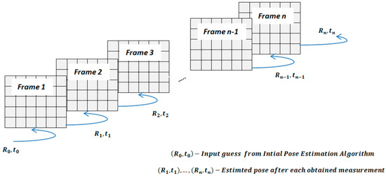
Figure 2. Frame-to-frame tracking of the target in the sequence of the depth or amplitude images. Each new frame is processed in order to find the estimate of the current target pose. The estimated pose is used as a guess in the following pose estimation.

2.2. Vision Based Navigation Using PMD Camera in DLR’s EPOS

At the present time we concentrate on investigating the potential application of the PMD sensor for future space missions. The development of this sensor started in the last two decades and preliminary on-ground validation tests showed promising results for space applications. To the best of our knowledge, this sensor has never been tested in space so far.

2.2.1. PMD Sensor Inside of the DLR-Argos 3D-P320 Camera

In this work we use the DLR-Argos 3D-P320 camera prototype (see Figure 3) provided by the Bluetechnix company (Wien, Austria). Its technical characteristics are summarized in Table 1.

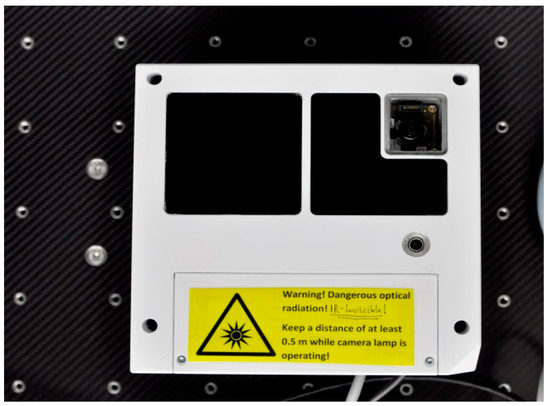
Figure 3. DLR-Argos 3D-P320 camera from Bluetechnix.

Table 1. Technical data of the PMD sensor inside the DLR-Argos 3D-P320 camera.

Field of View	28.91 × 23.45 deg
Resolution of the chip	352 × 287 pixels
Integration time	24 ms
Frames per second	45
Modulated frequencies	5.004 MHz, 7.5 MHz, 10.007 MHz, 15 MHz, 20.013 MHz, 25.016 MHz, 30 MHz
Mass/Power Consumption	2 kg/<25.5 W

2.2.2. PMD Working Principle

The modulated light from the 12 IR-flash LEDs emitted by the system is reflected on the scene’s surfaces and the reflected signal is captured by the sensitive array. Every pixel (i,j) on the array samples the amount of electrons $Q_1$,$Q_2$,$Q_3,Q_4$ measured at multiple time and locations. The phase shift of the signal acquired by the pixel (i,j) is calculated as [20]

$${\phi }_{ij}=\arctan \left(\frac{Q_3-Q_4}{Q_1-Q_2}\right).$$

(1)

Consequently, the depth $d_{ij}$ of the scene can be estimated pixelwise as

$$d_{ij}=\frac{c{\phi }_{ij}}{4\pi f_{\mathrm{mod}}}.$$

(2)

In Equation (2), $c$ denotes speed of light ($3\times {10}^8$ m/s), ${\phi }_{ij}$ is the measured phase shift at the pixel (i,j) and $f_{\mathrm{mod}}$ is the modulation frequency of the emitted signal. Having the raster depth image, it is possible to generate the 3D point cloud of the scene using the camera matrix.

Along with the range measurement, the PMD sensor provides co-registered amplitude data in every frame. The amplitude A of the received signal is defined as:

$$A_{ij}=\frac{\sqrt{{\left(Q_1-Q_2\right)}^2+{\left(Q_3-Q_4\right)}^2}}{2}.$$

(3)

The amplitude image can be represented as a 2D gray-scaled image [22] similarly to monocular vision. The amplitude image corresponds to the amount of the returning active light and presents the quality of the distance measurement. A high reflecting surface provides large amplitude values, scattering or less reflective surfaces cause low amplitudes. In particular, low amplitude suggests that a pixel has not received enough light to produce an accurate depth measurement [23]. In other words, the distance in every pixel is calculated regardless of amplitude [20]. Therefore, the amplitude value in a certain pixel can be obtained, while the depth value will be missing. This considerable feature of the PMD sensor allows getting the amplitude images independently from the depth images with more complete details of the scene. This is a prerequisite in order to create the hybrid navigation technique for the robust tracking of the spacecraft.

3. Hybrid Navigation Technique

In this paper, we propose a hybrid navigation technique that employs the advantages of two completely different tracking methods for model-based pose estimation of the uncooperative target during the close-range rendezvous. The proposed hybrid navigation technique employs a Computer-aided design CAD model of the target spacecraft, which can be assumed available in OOS and space debris removal missions. Furthermore, we assume that the initial pose of the target is known, as a-prior information for the tracker [24].

3.1. Spacecraft Model

In model-based pose estimation algorithms, the current pose of the target spacecraft is estimated by matching every new measurement of the sensor with a known simplified 3D model of the target created from its full CAD model.

In this paper, the test campaign for validating the pose estimation algorithms was performed in the DLR’s EPOS laboratory, whose target mockup is showed in Figure 4a. The mockup’s surface is partly covered by MLI material. Figure 4b illustrates the corresponding detailed CAD model of the mockup. The full CAD model contains 70,002 vertices. For the model-based pose estimations, we define two different shapes derived from the 3D CAD model. The first model, see on Figure 4c, is a 3D point cloud of the most significant geometric shapes of full CAD geometry, such as the hexagonal body and the frontal cone of the spacecraft. The number of points for this model was drastically reduced to 1200 in order to ensure onboard storage and rapid pose estimation with ICP. The second reference model used for pose estimation with amplitude images is a wireframe representation of the CAD geometry (see Figure 4d). The wireframe model represents the 3-dimensional object, by connecting the object’s vertices with straight lines or curves. In our case, the simple wireframe model inherits the shape of a spacecraft with its straight lines of the front hexagon and an additional extreme nose point.

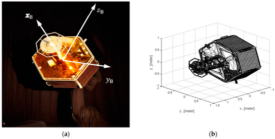
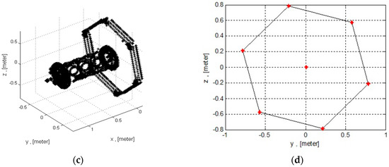
Figure 4. (a) The target mockup in German Aerospace Center (DLR)’s European Proximity Operations Simulator (EPOS) laboratory and the target principal frame B. (b) The original Computer-aided design (CAD) model of the target mockup. (c) 3D model with the most significant parts (cone nose and hexagon). (d) Wireframe model (hexagon and the extreme nose point).

The difference between shapes presented on Figure 4c,d is that the number of the key vertices for the algorithm with the depth images must be much more than for the algorithm with the amplitude images. Moreover, the straight lines presented in the second model will be needed for the further image processing procedure with the amplitude images.

The DLR’s EPOS facility allows realistic real-time close-range rendezvous simulation under realistic illumination conditions. Thereby the model appearance on the image can be different in every test case. These two shapes are sufficient only if we consider the navigation approach from to the frontal side of the target and when we assume that the target rotates around the x axis of the principal frame (illustrated in Figure 4a). For the other approach scenarios, which could be considered, e.g., rendezvous from the different sides, the shapes of the 3D model should contain other missing side parts in order to find the corresponding feature matches.

3.2. Autonomous Rendezvous Using 3D Depth Data

The model-based pose tracking of the target using known 3D geometrical shape of the object and the 3D locations of the features in every frame leads to a least squares minimization problem in order to find motion parameters [25]. The state-of-the art technique which is commonly adopted in 6 DoF 3D model-based tracking is the ICP algorithm [26]. This procedure iteratively finds the rigid transformation that aligns two three-dimensional shapes. In the case of uncooperative pose estimation, the two shapes are the 3D measured point cloud of the target object and the known 3D vertices of the model (Figure 4c). This method has shown its effectiveness in the real-time matching of misaligned 3D shapes, as well as robustness in the real-world application [12,27]. In order to ensure the real-time matching during the close approach, we employ a modified version of the classical ICP algorithm using the so-called “reverse calibration” for the nearest-neighbor search of corresponding points [28,29]. The term reverse calibration is explained in the paragraph 3.2.1. The organized point cloud from the raster image of the PMD sensor is the prerequisite to use this variation of the ICP algorithm.

3.2.1. Nearest Neighbor Search Using Reverse Calibration Technique

The most efficient way to search the point’s compatibility is inside of a limited space, i.e., only in a certain region of interest. This space can be determined by the search radius on the 2D area pointed from the source point. The search radius should be selected depending on the quality of the raster image, meaning that one can choose a small radius if the scene is presented quite completely. It will be sufficient to find the neighbors. However, when some data of the scene are missing, the radius should be increased in order to expand the nearest neighbor search area. Figure 5 depicts the illustration of this nearest neighbor search. Taking the point $a_i$ from the point set of the frame A and using the search radius, we can find at least one neighbor in the point set of the frame B. Here the term ‘reverse calibration’ is used intentionally because the follow task for the 2D circle determination around every interested point for the neighbor search can be solved by projection of the 3D point onto the image plane if a calibration matrix of the sensor chip is known. The PMD sensor of the DLR-Argos 3D-P320 camera has been calibrated according to [30], where the camera calibration matrix was accurately calculated using the DLR CalDe CalLab calibration toolbox [31].

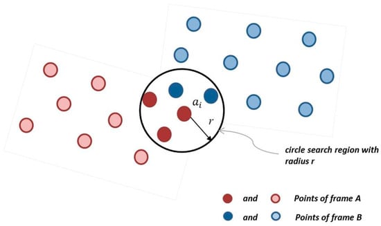
Figure 5. 2D neighbor search with a determined radius.

Every point $a_i$ from the point set of the frame A can be projected onto the image plane of the frame B, so the 2D point in a frame B in form of a pixel will be determined (see Figure 6). The obtained pixel with coordinates (i,j) indicates the starting point and the chosen radius determines the region of interests, where the nearest neighbor search should be conducted. The region of interest is defined symmetrically around the pixel (i,j). But in case of the points located near the sensors borders, the search area will be limited from one or another side by the absence of the pixels in an image area. In this case, the nearest neighbor will be absent.

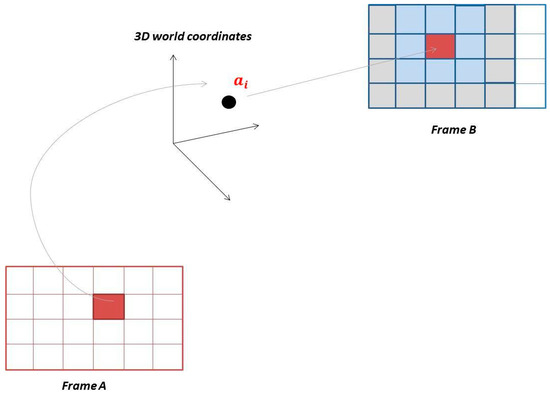
Figure 6. Projection of the 3D point to the image plane.

3.2.2. Estimation of Rigid Body Transformation via ICP

The pose estimation between two point sets for every frame i in a sequence of images can be calculated throughout transformations (${\mathit{R}}_i,{\mathit{t}}_i$), where ${\mathit{t}}_i$ is the relative position vector and ${\mathit{R}}_i$ is the rotation matrix.

The following main stages are included in the ICP routine in order to minimize point-to-point distance:

• The initial transformation (${\mathit{R}}_0,{\mathit{t}}_0$) provides the coarse alignment between the model and the target at a counter k = 0. It also narrows the search field for the neighbor points for the tracking algorithm.
• Nearest neighbor search by using reverse calibration technique with radius r.
• Finding correspondences between points from the frame A (e.g., points $a_j$, j = 1,…,N) and frame B (e.g., points $b_j$, j = 1,…,N).
• Compute the rotation ${\mathit{R}}_i$ and translation ${\mathit{t}}_i$ that minimize the point-to-point error function [32] in Equation 4 by using the corresponding points from the step 2

  $$\underset{\mathit{R},\mathit{t}}{\min }{\displaystyle \sum }_{j=1}^N\parallel {\mathit{b}}_j-{\left(\mathit{R}{\mathit{a}}_j+\mathit{t}\right)\parallel }^2,$$

  (4)
• The ICP algorithm terminates when the registration error is less than the predefined threshold value ${\theta }_{error}$, or when the number of iteration steps k is exceeded.

The ICP algorithm is an iterative process without guarantee that the optimization procedure will give converge to the global minima. Having reached the minimum may cause large errors in the expected pose of the target [19]. In general, the ICP solver is robust, but suffers from the following issues:

• Presented noise in measured and model point clouds.
• There is no perfect correspondence between measurement and model point. It means that the measured point will not be exactly the same point as a model.
• Initial guess, which causes incorrect correspondences between model and measured points.

In order to reach convergence to the local minima it is necessary to provide the accurate input by taking into account the above-mentioned problems. Notably, we assume the first guess for the first call of ICP available. In fact, a pose initialization routine can be employed to estimate the pose of the target spacecraft without guess [24].

3.3. Pose Estimation from 2D Gray-Scaled Images

Throughout the variety of the model-to-image registration techniques in computer vision using monocular cameras, we focus on designing the pose tracking technique based on feature correspondences between the 3D wireframe model and the detected features in the 2D image. The choice of the image features is a very important prerequisite for the accurate pose estimation. The image features are chosen during the mission design phase by considering simplicity and noise sensitivity in order to be recognizable in every image frame. Moreover, we need to keep in mind that even in cases when the depth data is partly lost and we still have only the redundant amplitude image information, the quality of the amplitude image can be restricted. The restriction appears because amplitude images contain also some occlusions, image noise and blur. These factors complicate the process of feature extraction, but do not prevent the pose estimation pipeline. Using the prior pose, the search space for the correct feature correspondence can be narrowed.

In this work we propose the model-to-image registration based on two types of low-level features: straight lines and points. We found this approach more reliable and robust when working with the existing mockup. Even under different environmental conditions, we try to distinguish and localize the edges of the spacecraft mockup, which are presented in form of straight lines and construct the hexagon. Furthermore, we try to recognize the central nose circle of the mockup, which should be visible by front side approach.

3.3.1. Image Processing

Amplitude images of PMD sensor reflect the strength of the signal received in each pixel of the sensor chip. The pixelwise amplitude information from the sensor is stored in a range from 0 to 255. Once a new image is acquired by the sensor, the edges of the mockup from the image are obtained using standard Canny edge [33] detection algorithm.

The next step is to employ the Hough transform technique to detect the target’s edges and central circle, which correspond to straight lines and circles on the image, respectively [34]. The target’s lines and the central circle are highlighted with a red color on Figure 7d. The Hough transform can be used in order to identify the parameters of a curve which best fits a set of given edge points. The shapes of the object in the image are detected by looking for the accumulating points in the parameter space. If the particular shape is presented in the image, then the mapping of all its points into parameter space and finding the local maxima must cluster around parameters values which correspond to that shape [34]. Computational capacity of the algorithm increases with the number of parameters which define the detected shape; for example, lines have two parameters and circles three.

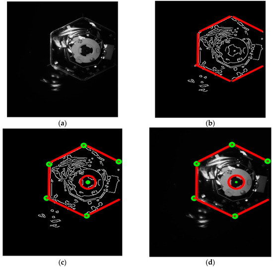
Figure 7. (a) 2D gray-scaled image from the amplitude channel. (b) Image with detected Canny edges and Hough Lines. (c) Image with detected Canny edges, Hough Lines and Hough Circle. (d) 2D gray-scaled image with detected Hough Lines and Hough Circle.

In summary, the line detection procedure consists of the following steps [35]:

• Low-pass filtering.
• Edge detection, e.g., using the Canny-edge detection, see Figure 7b.
• Mapping of edge points to the Hough space and storage in an accumulator.
• Interpretation of the accumulator to yield lines of infinite length.
• Conversion of infinite lines to finite lines, see on Figure 7c.

In order to generate a list of corrected feature pairs between the detected lines in the 2D image and the given lines of the 3D model, the known wireframe model is projected onto the image plane to a set of lines [36] using the pose solution obtained from the precedent pose estimation.

In some cases due to the space environmental illumination, the detected edges from the image can be partial and broken lines, merged lines or even completely wrong detected lines, which do not belong to the model. These inaccuracies can increase the number of feature correspondences between the lines in the image and the model [13]. Furthermore, it induces the incorrect motion estimation. To cope with this problem, a nearest neighbor search among detected lines from the Hough Transformation and the projected lines of the wireframe model lines is involved in the chain of image processing pipeline.

The line neighbor search is essentially important in order to reject the lines not belonging to the target’s edges. It is based on calculating the line differences in angle and position. The subset of lines that meets the threshold requirements is assumed to be correct. Presuming the straight line as a vector between a start and an end point, we can sum up the point-to-point correspondences of all the start and end points from the model and the image.

Along with the straight line detection technique using the Hough Line Transform, there is also the Hough Circle Transform technique for detecting circular objects in the image. The circle detection workflow is similar to the line detection described above. The key difference is the accumulator matrix, which returns the circles with three parameters: 2D coordinates of the position of the center and the radius of the circle. Accordingly, we try to detect central circle part at the end of the nose. The wrong detected circles, which do not belong to the original model, are eliminated from the image using the nearest neighbor search for the coordinates of the position of the center. If the distance between the detected central points is lower than the threshold, the detected circle is assumed to be correct. The center position of the circle is the additional key feature correspondence for the pose estimation.

3.3.2. Pose from Points

Once we obtain the correspondences between image and model points, we can solve the so-called Perspective-n-Point (PnP) problem to calculate the pose of the object with respect to the camera frame. There are several available solvers for the PnP estimation problem. The comparative assessment results for the different types of solvers are provided in the work of Sharma [37]. Based on the results of this research, we choose the Efficient Perspective-n-Points (EPnP) algorithm [38] due to its superior performance with respect to other solvers.

In order to determine position and orientation between a set of 2D image points ${\left\{{\mathit{q}}_i\right\}}_{i=1}^n$ and a set of 3D model points ${\left\{{\mathit{Q}}_i\right\}}_{i=1}^n$, we need to know the correspondences ${\left\{{\mathit{q}}_i\leftrightarrow {\mathit{Q}}_i\right\}}_{i=1}^n$. The key idea of EPnP is non-iterative method for computing camera coordinates of four virtual 3D control points ${\left\{{\mathit{Q}}_i^{\prime }\right\}}_{i=1}^4$. According to [39] ${\mathit{Q}}_1^{\prime }$ is the centroid of the 3D points ${\left\{{\mathit{Q}}_i\right\}}_{i=1}^n$. The other three control points are chosen as a set $\left\{{\mathit{Q}}_2^{\prime },{\mathit{Q}}_3^{\prime },{\mathit{Q}}_4^{\prime }\right\}$, which forms the basis aligned with the principal direction of ${\left\{{\mathit{Q}}_i\right\}}_{i=1}^n$. Each model point ${\mathit{Q}}_i$ and camera coordinate ${\mathit{Q}}_i^c$ can be expressed as follows

$${\mathit{Q}}_i={\displaystyle \sum }_{j=1}^4{\alpha }_{ij}{\mathit{Q}}_j^{\prime }\mathrm{and}{\mathit{Q}}_i^c={\displaystyle \sum }_{j=1}^4{\alpha }_{ij}{\mathit{Q}}_j^{\prime c}\mathrm{such}\mathrm{that}{\displaystyle \sum }_{j=1}^4{\alpha }_{ij}=1$$

(5)

In the Equation (5) a set ${\left\{{\mathit{Q}}_j^{\prime c}\right\}}_{j=1}^4$ refers to the camera coordinates of the control points.

Using this equation, which expresses the relationship between image coordinates and camera coordinates with known calibration matrix, we have ${\tilde{\mathit{q}}}_i\sim K{\mathit{Q}}_i^c=K{\displaystyle \sum }_{j=1}^4{\alpha }_{i,j}{\mathit{Q}}_j^{\prime c}$. The expanded form of previous expression yields to:

$$\left[\begin{array}{c}{q}_{ix}\\ q_{iy}\\ 1\end{array}\right]=\left[\begin{array}{c}{f}_1\\ 0\\ 0\end{array}\begin{array}{c}0\\ f_2\\ 0\end{array}\begin{array}{c}{c}_x\\ c_y\\ 1\end{array}\right]{\displaystyle \sum }_{j=1}^4{\alpha }_{ij}\left[\begin{array}{c}{\mathit{Q}}_{jx}^{\prime c}\\ {\mathit{Q}}_{jy}^{\prime c}\\ {\mathit{Q}}_{jz}^{\prime c}\end{array}\right]$$

(6)

After some algebraic manipulation, Equation (6) can be written in the following form:

$$\begin{array}{c}{\displaystyle \sum _{j=1}^4}{\alpha }_{ij}{f}_1{\mathit{Q}}_{jx}^{\prime c}+{\alpha }_{ij}\left(c_x-{\mathit{q}}_{ix}\right){\mathit{Q}}_{jz}^{\prime c}=0\\ {\displaystyle \sum _{j=1}^4}{\alpha }_{ij}{f}_2{\mathit{Q}}_{jy}^{\prime c}+{\alpha }_{ij}\left(c_y-{\mathit{q}}_{iy}\right){\mathit{Q}}_{jz}^{\prime c}=0\end{array}$$

(7)

Let us rewrite the above Equation (7) in a matrix form with unknowns ${\mathit{Q}}_i^{\prime c}$ and we get $\mathit{M}\mathit{Y}=0$, where M is a $2n\times 12$ sized matrix and $\mathit{Y}={\left[{\mathit{Q}}_{1x}^{\prime c},{\mathit{Q}}_{1y}^{\prime c},{\mathit{Q}}_{1z}^{\prime c},{\mathit{Q}}_{2x}^{\prime c},\dots {\mathit{Q}}_{4z}^{\prime c}\right]}^T$ is $12\times 1$ vector of unknown camera coordinates of 3D points which we want to compute. Here $Y$ is linear combination of singular vectors $\left\{Y_{\mathrm{i}}\right\}$ corresponding to right null space of M, $Y={{\displaystyle \sum }}^{\text{}}{\mathsf{\beta }}_{\mathrm{i}}{Y}_{\mathrm{i}}$. These singular vectors are the eigenvectors of $12\times 12$ matrix $M^{\mathrm{T}}M$. Therefore, in order to obtain the camera coordinates $Q_{\mathrm{i}}^{\mathrm{c}}$, we need to compute the coefficients ${\mathsf{\beta }}_{\mathrm{i}}$. Detailed description how to find the coefficients ${\mathsf{\beta }}_{\mathrm{i}}$ is presented in the paper of Lepetit et al. [38].

4. Results

The proposed hybrid navigation technique was tested offline on two datasets of images recorded in two different rendezvous scenarios simulated in DLR’s EPOS laboratory. The overall positioning accuracy of the EPOS facility is 1.56 mm (position) and 0.2 deg (orientation) [21]. The algorithms proposed in this paper were implemented in C++, using OpenCV [40] library for straight line and central circle detection.

In the first scenario, we considered a frontal approach at a certain angle to an attitude-stabilized target. Figure 8 shows the first dataset of depth and amplitude images acquired during this simulated maneuver. In the second scenario, we considered a straight frontal approach to a target tumbling about its X axis (see Figure 4) at a rate of 5 deg/s. The second dataset of depth and amplitude images acquired during this maneuver is shown in Figure 9. Initial distance for both approach scenarios was 7 m. Overall, every data set consists of 20 images. For every test image acquired by the simulator, the ground truth between camera and the mockup was logged by EPOS.

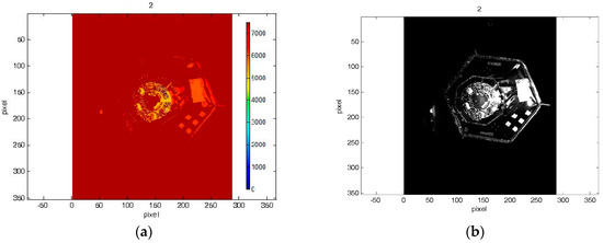
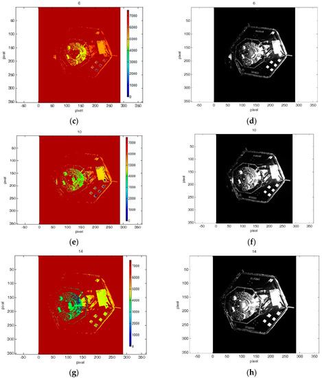
Figure 8. (a–h) Some depth and amplitude images from the first dataset.

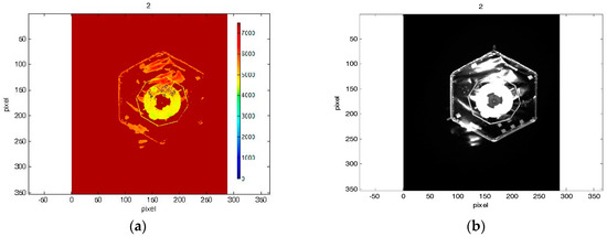
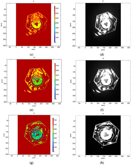
Figure 9. (a–h) Some depth and amplitude images from the second dataset.

Figure 8 and Figure 9 highlight the fact that amplitude and depth images, which were acquired at the same instants, present some differences. In most cases, the amplitude image reflects most of the visible contours, whereas on the depth image no information of some edges is available.

The experimental campaign, which we considered in this paper, is as follows. The pose estimation using the ICP with reverse calibration algorithm (detailed explanation is provided in Section 3.2.1 and Section 3.2.2) is primary conducted. The image processing procedure, which is described in Section 3.2.1 and Section 3.2.2, has been run thereafter for the amplitude images. After processing the output results from the obtained depth images, we have revealed and shown how the redundant algorithm with the amplitude images can (partly) compensate and/or provide more accurate estimations of the complete pose, when the algorithm with the depth images provides inaccurate estimated pose.

4.1. ICP-Based Pose Estimation from PMD Depth Images

For the ICP with reverse calibration, we varied the radius for the 2D neighbor search. The radius was defined in a range from 10 to 50 pixels. In Table 2, the Root Mean Square (RMS) errors and the processing time are presented for both sequences of images after appliance of ICP with the reverse calibration.

Table 2. Root Mean Square (RMS) errors and average computational time for Iterative Closest Point algorithm (ICP) with reverse calibration.

First Set of Images, Target not Rotating
Radius for the Neighbor Search	10	15	20	25	30	35	40	45	50
RMS (Roll), deg	4.050	3.102	3.08	2.59	2.38	2.58	2.69	2.82	2.51
RMS (Pitch), deg	5.822	1.463	4.71	3.96	3.744	3.081	5.134	2.91	3.52
RMS (Yaw), deg	2.232	2.024	2.58	2.308	2.44	1.044	2.02	2.36	2.10
RMS (X), m	0.077	0.106	0.08	0.088	0.086	0.06	0.074	0.058	0.077
RMS (Y), m	0.375	0.056	0.04	0.045	0.045	0.04	0.047	0.031	0.038
RMS (Z), m	0.157	0.182	0.11	0.096	0.100	0.08	0.117	0.087	0.088
CPU time, sec	2.1	2.3	2.5	2.6	2.9	3	3.1	3.3	3.5
Second Set of Images, Rotating Target
Radius for the Neighbor Search	10	15	20	25	30	35	40	45	50
RMS (Roll), deg	3.068	6.84	8.78	5.31	3.59	4.31	5.66	7.20	4.83
RMS (Pitch), deg	5.29	5.94	4.46	5.56	3.44	7.05	3.90	4.59	6.64
RMS (Yaw), deg	1.94	1.83	1.33	0.526	1.81	1.103	1.94	1.81	1.24
RMS (X), m	0.099	0.16	0.20	0.15	0.104	0.177	0.12	0.150	0.126
RMS (Y), m	0.089	0.109	0.113	0.092	0.077	0.07	0.109	0.116	0.166
RMS (Z), m	0.05	0.046	0.046	0.039	0.048	0.034	0.037	0.044	0.039
CPU time, sec	3.1	3.45	3.8	4.2	4.6	5	5.4	5.8	6

The demanded central processing unit (CPU) times for processing one image for the both data sets are also presented in Table 2. Considering the results from the recorded datasets of the images, it could be noticed that the radius of the neighbor search influences the position errors. It is connected with the obtained data from the sensor. If some depth data of the mockup are absent on the image, no neighbor points could be found for some points of the projected model. Besides that, some incorrect information could be presented on the image, e.g., high reflection from the target can create additional areas of the depth, which in reality does not exist. It evidently can be observed on the Figure 9 in the images 5, 7 and 9.

Therefore, the low number of point correspondences or mismatches between scene and model points can lead to the incorrect estimation of the pose. In general, the good case with low RMS position errors could be found throughout the whole simulated results both for the first and for the second datasets. For example, if the radius for 2D neighbor search for the non-rotated target is in a range of 25, 30 and 35, the RMS errors for the rotation components do not exceed 4 degrees and the RMS errors for the translation components are in the range less than 10 cm. For the rotated target, because of the quite large number of outliers and completely absent depth information from one side of the mockup in the first depth images, the translation RMS errors along the X axis are high almost in all simulated cases. However, if the radius is equal 10, 25 and 30 pixels the RMS errors for the rotation components do not exceed 7.05 degrees and the RMS errors for the translation components are less than 15 cm. In fact, input for the pose estimation algorithm with depth images is the raw depth data without depth correction algorithm. Therefore, we assume that the RMS errors for the radiuses 10, 25 and 30 are acceptable, knowing that they include not only the errors from pose estimation algorithms.

Let us consider the detailed errors of pose estimation for every depth image when the radius of the neighbor search is equal 25 pixels. On Figure 10, the norm of angular and translation errors are presented for the attitude–stabilized and for the tumbling target over time. The spots in a form of error spikes on these two plots (e.g., images 15, 17, 19 for the first data set and images 4, 7 and 9 for the second data set) indicate the moments when the error of estimated pose with depth image is very high. For the first scenario, these peaks have been caused by position of the stabilized target, as the left part of the spacecraft was hardly observed. For the second dataset, peaks of errors have arisen since the target was tumbling, causing severe reflections from the surface. Therefore, in the next section we show the results for the same data sets the EPnP-based pose estimation technique on the amplitude images in order to investigate how to overcome these peaks of pose error.

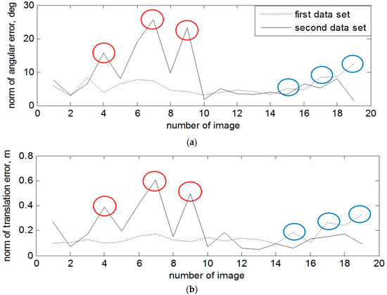
Figure 10. (a) Norm of angular error for the attitude-stabilized and rotated target with ICP-based technique and radius for neighbor search 25 pixels. (b) Norm of translation error for the attitude-stabilized and rotated target with ICP-based technique and radius for neighbor search 25 pixels.

4.2. Pose Estimation with the Amplitude Image from PMD Sensor

We now test the supplementary EPnP-based pose estimation technique on the amplitude images of the two datasets. In particular, we want to investigate when this technique can overcome the peaks of error generated by the ICP-based pose estimation algorithm. This comparison is performed by considering the results of the ICP-based algorithm with search neighbor radius of 25 pixels.

Because of the shape of the mockup (see Figure 4), we can get only a limited amount of the endpoints from the detected lines (see explanation in Section 3.3.1). As shown in Figure 7, the maximum number is 7 points: 6 intersected points or corners of the hexagon along with the center of the central circle. Since not all the feature points can be detected in every frame, we just run the algorithm for that number of points which was available after image processing.

On Figure 11 and on Figure 12, the norms for rotation and translation errors of pose estimation are individually shown for each depth and amplitude image. The red marking on both Figures shows the cases when the algorithm with the amplitude images shows better results by estimating pose than ICP with the depth images. The average central processing unit CPU time to process one amplitude image is about 1 s.

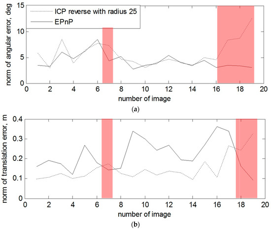
Figure 11. (a) Norm of angular error for every amplitude and distance image for the first data set. (b) Norm of distance error for every amplitude and distance image for the first data set.

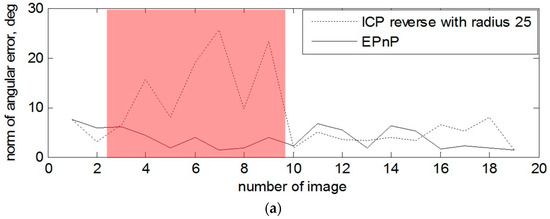
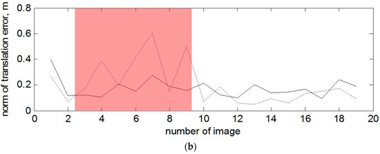
Figure 12. (a) Norm of angular error for every amplitude and distance image for the second data set. (b) Norm of distance error for every amplitude and distance image for the second data set.

From the results in Figure 11, we can determine that, in the case of the non-rotated target, the errors for estimated orientation using the EPnP-based pose estimation technique (images 7, 18 and 19) are lower. In Table 3, the error norms for rotation and translation are presented for the mentioned images.

Table 3. Norms of translation and rotation errors for the stabilized target of the first dataset.

Norms of Translation Error, Meter
Image	7	18	19
ICP-based technique	0.16	0.26	0.32
EPnP technique	0.13	0.18	0.11
Norms of Attitude Error, Degrees
Image	7	18	19
ICP-based technique	7.68	8.33	12.46
EPnP technique	4.8	3.89	2.99

These errors are due to the approaching scenario. The closer the target was, the less the front left part was visible and the central circle part could not be fully detected correctly. The Figure 13 shows the 7th depth and amplitude images from the first data set, where the EPnP outperforms the ICP with reverse calibration in the form of calculation of the rotation and translation components, because of the missed depth data of the left upper and lower parts of the mockup in the depth image.

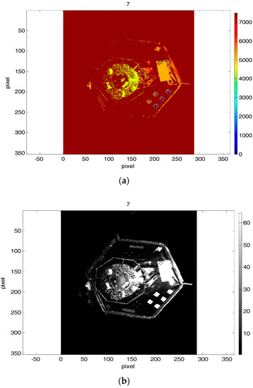
Figure 13. Subfigure (a) depicts 7th depth image and subfigure (b) contains the 7th amplitude image from the first data set, where the EPnP outperforms the ICP with reverse calibration in form of calculation of the rotation and translation components.

In the case with the rotating target and when the depth measurement of the right part of the mockup are also absent at the beginning of the tracking, one can observe a sufficient advantage of using 2D amplitude images for the estimation of the rotation and also some of the translation components. For example, the most obvious example is presented on Figure 12 and image 4, 7 and 9.

The 7th depth and amplitude images from the second data set are depicted on Figure 14, as it was made for the first scenario. The norms of attitude and position errors for the mentioned images with the ICP-based technique and the EPnP technique are presented in Table 4.

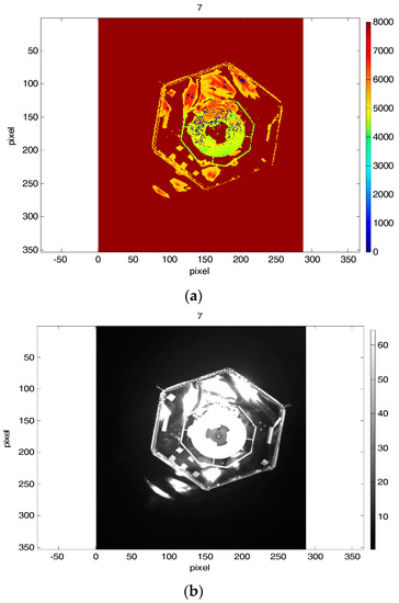
Figure 14. Subfigure (a) depicts the 7th depth image and subfigure (b) contains the 7th amplitude image from the second data set, where the EPnP outperforms the ICP with reverse calibration in form of calculation of the rotation and translation components.

Table 4. Norms of translation and rotation errors for the tumbling target in the second dataset.

Norms of Translation Error, Meter
Image	4	7	9
ICP-based technique	0.39	0.6	0.49
EPnP technique	0.10	0.277	0.15
Norms of Attitude Error, Degrees
Image	4	7	9
ICP-based technique	15.73	25.91	23.27
EPnP technique	4.72	4.35	2.7

The monocular vision overcomes the performance of the algorithm with depth images due to the higher quality of the amplitude images. The depth images were strongly corrupted by the absence of the depth data.

5. Discussion and Conclusions

A hybrid navigation technique for tracking the pose of an uncooperative target spacecraft during close range rendezvous has been proposed in this paper. The key innovation of this technique is the usage of two different pose estimation approaches to ensure robustness in the tracking procedure even under harsh illumination conditions. This is possible since the PMD sensor provides two types of measurement at the same time: one depth image and one amplitude image, which is analogous to a gray scale image. The first method for pose tracking is the ICP algorithm with reverse calibration, which determines the current pose by matching the measured point cloud with a reference 3D model of the spacecraft. The second technique employs the Hough algorithm to detect the target’s true edges in the amplitude image as straight lines. Subsequently, the endpoints are matched with the corresponding vertexes of the 3D model. Finally, the EPnP solver estimates the current pose of the target spacecraft using these point correspondences.

The main advantage of the proposed technique is the software redundancy by using the measurements of the PMD sensor without hardware redundancy. This redundancy is crucial to ensure robustness of the tracking procedure. In fact, the test campaign using realistic sensor data from DLR’s European Proximity Operation Simulator facility showed that the ICP routine produced some inaccurate estimates. These errors were originated by the corrupted depth images caused by the intense light reflection on the target’s surface that saturates the sensor’s pixels. To ensure precise pose tracking, we cannot rely on the depth measurements only. In case of problems, it is necessary to use the additional pose estimation technique based on the EPnP algorithm and the amplitude images.

It turned out that that the amplitude measurements provide an accurate 2D image of the spacecraft algorithm under the same illumination conditions as in the case with depth measurements, allowing precise pose estimation using the image processing and EPnP. With these results, we proved the necessity to adapt the pose estimation pipeline to the sun illumination and we demonstrate the potential usage of the proposed techniques in one unique hybrid navigation system. The proposed improvement will increase the accuracy and robustness of the navigation system to keep tracking the target with the PMD camera. We are interested in the further combination of the best measurements from the pose estimation techniques in order to get the final one pose. This solution should balance the pros and cons of the proposed completely different techniques, based on the experience obtained during the test simulation with real data. Throughout different techniques for the fusion of the state estimates, we would consider the Kalman filter as a typical one applied in visual tracking applications.

Potentially, it is necessary to test the hybrid navigation technique for different test scenarios, e.g., by simulation of a sun illumination from different directions or by choosing another approach scenario with other visible parts of the mockup, which have other shapes and types of material.

References

- Fehse, W. Automated Rendezvous and Docking of Spacecraft; Cambridge Aerospace Series; Cambridge University Press: Cambridge, UK, 2003. [Google Scholar]
- Merriaux, P.; Dupuis, Y.; Boutteau, R.; Vasseur, P.; Savatier, X. Robust Robot Localization in a Complex Oil and Gas Industrial Environment. J. Field Robot. 2017. [CrossRef]
- Ballantyne, J.; Johns, E.; Valibeik, S.; Wong, C.; Yang, G.Z. Autonomous Navigation for Mobile Robots with Human-Robot Interaction. In Robot Intelligence. Advanced Information and Knowledge Processing; Springer: London, UK, 2010. [Google Scholar]
- Biswajit, S.; Prabir, K.P.; Debranjan, S. Building maps of indoor environments by merging line segments extracted from registered laser range scans. Robot. Auton. Syst. 2014, 62, 603–615. [Google Scholar]
- Lakaemper, R. Simultaneous Multi-Line-Segment Merging for Robot Mapping Using Mean Shift Clustering. In Proceedings of the Intelligent Robots and Systems (IROS), St. Louis, MO, USA, 10–15 October 2009. [Google Scholar]
- Pozna, C.; Precup, R.E.; Földesi, P. A novel pose estimation algorithm for robotic navigation. Robot. Auton. Syst. 2015, 63, 10–21. [Google Scholar] [CrossRef]
- Inaba, N.; Oda, M. Autonomous Satellite Capture by a Space Robot. In Proceedings of the IEEE International Conference on Robotics and Automation, San Francisco, CA, USA, 24–28 April 2000. [Google Scholar]
- Howard, R.T.; Heaton, A.F.; Pinson, R.M.; Carington, C.K. Orbital Express Advanced Video Guidance Sensor. In Proceedings of the IEEE Aerospace Conference, Big Sky, MT, USA, 1–8 March 2008. [Google Scholar]
- Naasz, B.; Eepoel, J.V.; Queen, S.; Southward, C.M.; Hannah, J. Flight results of the HST SM4 Relative Navigation Sensor System. In Proceedings of the 33rd Annual AAS Guidance and Control Conference, Breckenridge, CO, USA, 6–10 February 2010. [Google Scholar]
- Opromolla, R.; Fasano, G.; Rufino, G.; Grassi, M. A review of cooperative and uncooperative spacecraft pose determination techniques for close-proximity operations. Prog. Aerosp. Sci. 2017, 93, 53–72. [Google Scholar] [CrossRef]
- Opromolla, R.; Fasano, G.; Rufino, G.; Grassi, M. Uncooperative pose estimation with a LIDAR-based system. Acta Astronaut. 2015, 10, 287–297. [Google Scholar] [CrossRef]
- Ventura, J. Autonomous Proximity Operations to Noncooperative Space Target. In Proceedings of the Deptment of Mechanical Engineering, Orlando, FL, USA, 30 January 2005–1 February 2017. [Google Scholar]
- D’Amico, S.; Benn, M.; Jørgensen, J.L. Pose Estimation of an Uncooperative Spacecraft from Actual Space Imagery. Int. J. Space Sci. Eng. 2014, 2, 171–189. [Google Scholar]
- Oumer, N.W. Visual Tracking and Motion Estimation for an On-Orbit Servicing of a Satellite. Ph.D. Thesis, University of Osnabruck, Osnabruck, Germany, 2016. [Google Scholar]
- Benninghoff, H.; Rems, F.; Boge, T. Development and hardware-in-the-loop test of a guidance navigation and control system for on-orbit servicing. Acta Astronaut. 2014, 102, 67–80. [Google Scholar] [CrossRef]
- Oumer, N.W.; Panin, G. 3D Point Tracking and Pose Estimation of a Space Object Using Stereo Images. In Proceedings of the 21st International Conference on Pattern Recognition (ICPR 2012), Tsukuba, Japan, 11–15 November 2012. [Google Scholar]
- Ringbeck, T.; Hagebeuker, B. A 3D Time of Flight Camera for object detection. In Optical 3D Measurement Technologies; ETH Zürich: Zürich, Switzerland, 2007. [Google Scholar]
- Tzschichholz, T. Relative Pose Estimation of Known Rigid Objects Using a Novel Approach of High-Level PMD-/CCD-Sensor Data Fusion with Regard to Application in Space. Ph.D. Thesis, University of Würzburg, Würzburg, Germany, 2014. [Google Scholar]
- Ventura, J.; Fleischner, A.; Walter, U. Pose Tracking of a Noncooperative Spacecraft during Docking Maneuvers Using a Time-of-Flight Sensor. In Proceedings of the AIAA Guidance, Navigation, and Control Conference (AIAA SciTech Forum), San Diego, CA, USA, 4–8 January 2016. [Google Scholar]
- Dufaux, F.; Pesquet-Popescu, B.; Cagnazzo, M. Emerging Technologies for 3D Video: Creation, Transmission and Rendering; John Wiley & Sons, Ltd.: London, UK, 2013. [Google Scholar]
- Benninghoff, H.; Rems, F.; Risse, E.A.; Mietner, C. European Proximity Operations Simulator 2.0. (EPOS)-A Robotic-Based Rendezvous and Docking Simulator. J. Large-Scale Res. Facil. 2017, 3. [Google Scholar] [CrossRef]
- Fuchs, S.; Hirzinger, G. Extrinsic and depth calibration of ToF-cameras. In Proceedings of the 22nd IEEE Conference Computer Vision Pattern Recognition, Anchorage, AK, USA, 23–28 June 2008. [Google Scholar]
- Reynolds, R.; Dobos, J.; Peel, L.; Weyrich, T.; Brostow, G.J. Capturing time-of-flight data with confidence. In Proceedings of the IEEE Conference on Computer Vision and Pattern Recognition (CVPR), Colorado Springs, CO, USA, 20–25 June 2011. [Google Scholar]
- Klionovska, K.; Benninghoff, H. Initial pose estimation using PMD sensor during the rendezvous phase in on-orbit servicing missions. In Proceedings of the 27th AAS/AIAA Space Flight Mechanics Meeting, San Antonio, TX, USA, 5–9 February 2017. [Google Scholar]
- Or, S.H.; Luk, W.S.; Wong, K.H.; King, I. An efficient iterative pose estimation algorithm. Image Vis. Comput. 1998, 16, 353–362. [Google Scholar] [CrossRef]
- Besl, P.J.; Mckay, N.D. A method for registration of 3D shapes. IEEE Trans. Pattern Anal. Mach. Intell. 1992, 14, 239–256. [Google Scholar] [CrossRef]
- Pomerlau, F.; Colas, F.; Siegwart, R.; Magnenat, S. Comparing ICP Variants on Real world Data Sets. Auton. Robot. 2013, 34, 133–148. [Google Scholar] [CrossRef]
- Blais, G.; Levine, M. Registering multiview range data to create 3D computer objects. IEEE Trans. Pattern Anal. Mach. Intell. 1995, 17, 820–854. [Google Scholar] [CrossRef]
- Levoy, M.; Rusinkiewicz, A. Efficient variants of the icp algorithm. In Proceedings of the 3rd International Conference on 3D Digital Imaging and Modeling, Quebec City, QC, Canada, 28 May–1 June 2001. [Google Scholar]
- Klionovska, K.; Benninghoff, H.; Strobl, K.H. PMD Camera-and Hand-Eye Calibration for On-Orbit Servicing Test Scenarios on the Ground. In Proceedings of the 14th Symposium on Advanced Space Technologies in Robotics and Automation (ASTRA), Leiden, The Netherlands, 20–22 June 2017. [Google Scholar]
- DLR CalDe and DLR CalLab. Available online: http://www.robotic.dlr.de/callab/ (accessed on 25 October 2017).
- Horn, B.K.P. Closed-form solution of absolute orientation using unit quaternions. J. Opt. Soc. Am. 1987, 4, 629–642. [Google Scholar] [CrossRef]
- Canny, J. A Computational Approach to Edge Detection. Read. Comput. Vis. 1987, 184–203. [Google Scholar] [CrossRef]
- Amtonovic, D. Review of the Hough Transform Method, with an Implementation of the Fast Hough Variant for Line Detection; Department of Computer Science, Indiana University: Bloomington, IN, USA, 2008. [Google Scholar]
- Available online: http://web.ipac.caltech.edu/staff/fmasci/home/astro_refs/HoughTrans_lines_09.pdf (accessed on 15 October 2017).
- Cropp, A.; Palmer, P. Pose estimation and relative orbit determination of nearby target microsatellite using passive imagery. In Proceedings of the 5th Cranfield Conference on Dynamics and Control of Systems and Structures in Space, Cambridge, UK, 14–18 July 2002. [Google Scholar]
- Sharma, S.; D’Amico, S. Comparative assessment of techniques for initial pose estimation using monocular vision. Acta Astronaut. 2016, 123, 435–445. [Google Scholar] [CrossRef]
- Lepetit, V.; Moreno-Noguer, F.; Fua, P. EPnP: An Accurate O(n) Solution to the PnP Problem. Int. J. Comput. Vis. 2009, 81, 155–166. [Google Scholar] [CrossRef]
- Bhat, S. Visual words for pose estimation. In Signal and Image Processing; Universite de Lorraine: Lorraine, France, 2013. [Google Scholar]
- OpenCV. Available online: http://opencv.org/ (accessed on 25 October 2017).
© 2018 by the authors. Licensee MDPI, Basel, Switzerland. This article is an open access article distributed under the terms and conditions of the Creative Commons Attribution (CC BY) license (http://creativecommons.org/licenses/by/4.0/).