1. Introduction
Mobile robots traveling across off-road terrains constitutes a challenging research field mainly owing to the issue of robot mobility, which greatly depends on the terrain type, the running gear-terrain interaction, and the own soil properties [
1,
2]. Path planning and motion control strategies must take “non-geometrical” obstacles of the terrain ahead of the robot into account in order to successfully achieve a desired waypoint or goal. For example, a longer path on compact soil would be preferable to a shorter path on loose sandy soil because the traction characteristics of sandy soil are poorer than those found on compact soil [
2].
It is true that several terrain parameters can be roughly known
a priori for a specific soil obtained from offline estimation using dedicated equipment. However, in practice, off-road terrains leak homogeneity, having different subregions with different terrains and, hence, different properties [
1,
3,
4]. Identifying the forthcoming terrain leads to reducing the risk of robot immobilization and increasing the performance of the path planner and motion controller. These circumstances mean that off-road robotic applications must predict the type of the diverse terrains ahead of the robot
online.
The research addressed in this paper is framed within the context of predicting the type of the forthcoming terrain. The main contribution lies in combining information obtained from one downward-looking camera with the frontal view of the environment obtained with a forward-looking camera. Firstly, an SVM model is used to classify the terrain just beneath the robot (ground images). This information is then combined with a color-based classifier that deals with frontal images. Notice that the original frontal view is split into a set of subimages or patches, and terrain classification is referred to each particular patch. We can thus detect multiple types of terrains in one single image.
The rest of the paper is organized as follows. Previous work is reviewed in
Section 2. In
Section 3, a general overview of the proposed methodology is described and the testbed and the dataset of images used in this research are presented.
Section 4 explains the Gist-based classifier used to classify the terrain beneath the robot. The Gist descriptor and the SVM training methodology are also described. The color-based classifier and the rectification strategy dealing with frontal images are both discussed in
Section 5.
Section 6 deals with the proposed procedure to improve the former color-based classification by combining ground and frontal images.
Section 7 provides experimental results of the proposed approach.
Section 8 concludes the paper and outlines future research.
2. Related Work
Firstly we review some approaches found in the literature using simplified models and propioceptive sensors for terrain classification and characterization. In [
5] a set of equations based on the Mohr-Coulomb criterion is arranged such that terrain cohesion and internal friction angle are both estimated from measurable data (mainly from propioceptive sensors). In [
6] an approach based on experimental data is used to correlate motor currents and the angular rate of the robot with soil parameters (slip and coefficient of motion resistance). In [
7] a Bayesian multiple-model estimation methodology for identifying terrain parameters from estimated terrain force and slip characteristics is presented. A method to classify a terrain based on vibrations induced in the robot structure by wheel-terrain interaction is addressed in [
8]. Vibrations sensed online (by means of a contact microphone mounted on the wheel frame) are classified based on their similarity to vibrations observed during an offline supervised training phase. A similar approach is proposed in [
9]. In this case, acoustic data from microphones are labeled and used offline to train a supervised multiclass classifier that can be applied to classify vehicle-terrain interactions. Additionally, a downward-looking camera collects images which assists in hand-labeling. The main feature of these strategies is that they use a set of propioceptive sensors, and no actual information is obtained from the terrain. This means the terrain is classified according to how the robot behaves in response to the features or the interaction with the terrain. The main drawback of these approaches is that there is no prediction ability, which could ultimately lead to the robot becoming trapped.
In order to increase the applicability of propioceptive-based methods and to increase the predictive abilities of the robot, it is interesting to consider exteroceptive sensors. Some approaches take advantage of vision or range data to classify a terrain from a distance. The pioneering work in [
10] describes both a stereo-based obstacle detection and a terrain cover color-based classification. Combining this information, each point in the scene is classified as a “material class” in a predetermined family. This class outlines the traversability characteristics of the terrain. This work is reviewed and improved in [
11] by adding a laser rangefinder sensor. This approach was successfully tested in vegetated terrain. These strategies motivated the work in [
3], in which an approach to predict slip from a distance using stereo imagery is proposed. To address this issue, terrain appearance and geometry information are correlated with the measured slip. This relationship is learned using a receptive field regression approach. In the end, slip is predicted online remotely from visual information only (terrain slopes). This solution was integrated into a slip-compensation navigation architecture in [
12]. In this paper, the path planning stage is performed over a slip-augmented goodness map resulting in optimal routes that avoid geometric and non-geometric hazards. The utility of combining propioceptive sensors (e.g., IMU and motor current) with a stereo camera to extend terrain classification from near to far distance is also demonstrated in [
13]. In this case, a short-range local terrain classifier and a long-range image-based classifier are properly combined and run in real-time. The main conclusion regarding vision-based classification is that almost all the references deal with forward-looking cameras. There are two important issues here: (1) the forward-looking camera is further from the ground than the downward-looking camera; (2) images are subject to perspective distortion. These two facts may lead to featureless regions in the image, and ultimately to misclassification. Notice that a downward-looking camera is parallel to the ground. It therefore offers finer images and, hence, the probability of misclassification is much smaller.
At this point, we review the state-of-the-art in terms of downward-looking cameras. The motivation of using one downward-looking camera in this research comes from [
14,
15]. In [
14], a combination of four optical mouse sensors -and an INS-GPS module- is employed to perform visual odometry for a lunar rover. The vision module is mounted under the vehicle facing downwards, and it reports lateral motion velocities. In [
15], a downward-looking camera is employed for estimating the motion of a car-like robot. In this case, a visual odometry method based on template matching is used. The performance of the method is validated in several outdoor environments. The work in [
16] presents a downward-looking stereo camera for estimating the robot velocity. This stereo system permits the height variation existing in non-flat terrains to be compensated for. A smart solution for increasing the applicability of downward-looking cameras to uneven terrain conditions appears in [
17,
18]. In particular, a telecentric lens is inserted in front of the camera head. This lens creates a telecentric optical system that provides a constant image scale factor regardless of the distance between the lens and the ground. In [
19] a novel method for sideslip estimation is proposed. In particular, it is based on using a rearward-facing camera to measure the pose of the trace that is produced by the wheels, and detects whether the robot follows the desired path or deviates from it because of slippage.
The main conclusion drawn from this review is that although the use of downward-looking cameras is not new in robotics, especially in the field of micro-aerial robots, there are few papers describing the use of such cameras in off-road “wheeled” mobile robotics. As shown, these publications are mainly devoted to estimating vehicle-terrain parameters or to estimating the robot’s position. To the best of the authors’ knowledge, this is the first time that a downward-facing camera is used for automatic terrain classification in off-road conditions (quasi-planar terrains).
3. General Framework for Terrain Classification
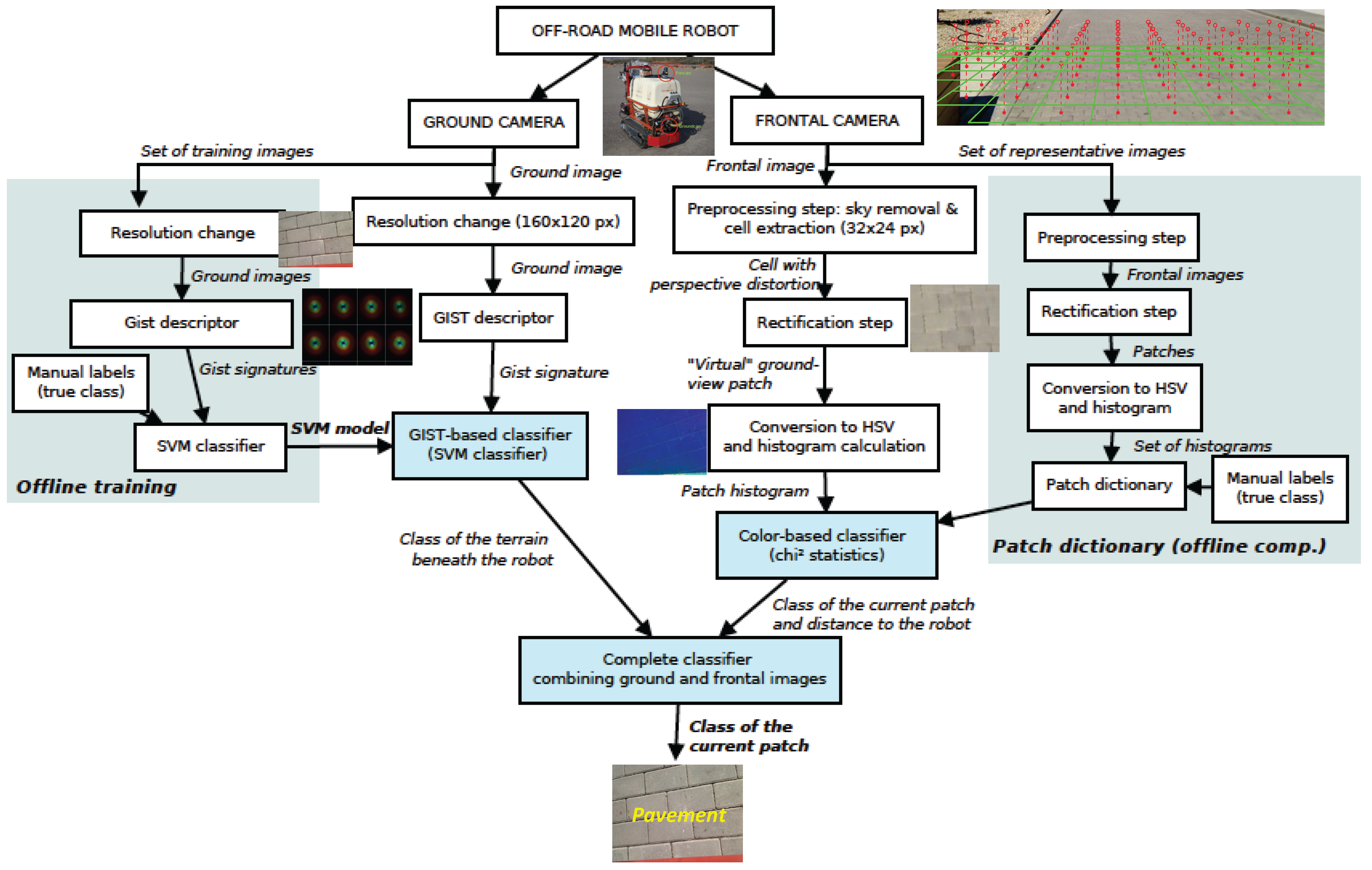
This section gives a global view of the proposed framework to classify a given (heterogeneous) terrain (
Figure 1). Initially, two different approaches are followed depending on the images used (ground camera or frontal camera). Regarding the ground images, we firstly resize the images. This is mainly to reduce computation time (recall that image classification is carried out online). In any case, the new resolution offers a performance similar to that achieved with the original images (see
Section 7.1). Subsequently, a Support Vector Machine (SVM) classifier is trained using a set of Gist-descriptor signatures and a hand-labeled vector stating the class of each image (see a typical Gist-descriptor signature in
Figure 4). Notice that at query time, this SVM classifier provides the class of the terrain appearing in the ground image. Details about the Gist descriptor and the SVM are given in
Section 4.
On the other hand, images taken with the frontal camera are classified according to their color. First a set of subimages or patches is obtained, that is, texture elements. These patches are not square and have a “perspective deformation”. We apply a rectification step (by means of a homography) in order to obtain rectangular patches with no perspective deformation, referred to as rectified patches. After that, the images are converted to HSV color space and the histogram of a set of representative images is saved in a database together with a hand-labeled vector defining the class of each histogram. At query time, each new rectified patch is compared with these values in order to obtain the corresponding class. The color-based classifier is detailed in
Section 5.
Finally, the former color-based classification of the rectified patches is improved by considering information from the ground images (see
Section 6).
Before proceeding to explain in detail the contribution of this work, we would like to highlight the main limitations and assumptions of the proposed framework and the possible solutions:
We assume that the terrain beneath the robot and captured by the downward-looking camera is the same for both tracks. This means that only one terrain type is beneath the robot at each sampling instant. This issue has been validated experimentally, that is, the current field of view of the downward-looking camera is small enough to guarantee that it always captures one single type of terrain at once.
The combination of the two classifiers mainly improves the result of the frontal rectified patches that are correlated with the terrain underfoot. This means the rectified patches that belong to the same class as that identified by the Gist-based classifier are correctly classified in case of misclassification. A preliminary solution to this point consists of the implementation of a filter considering the 7-neighbors of each patch (see
Section 6). Our future research will consider including new sensors such as a LIDAR sensor or a second frontal camera. However, we would like to remark that this solution would increase computation time which might prevent its applicability in fast systems or in systems with low performance computers.
It is assumed that the robot is moving on a quasi-planar terrain (e.g., flat terrain, flat sloped terrain). This is because the distance between the downward-looking camera and the ground should remain constant.
3.1. Testbed
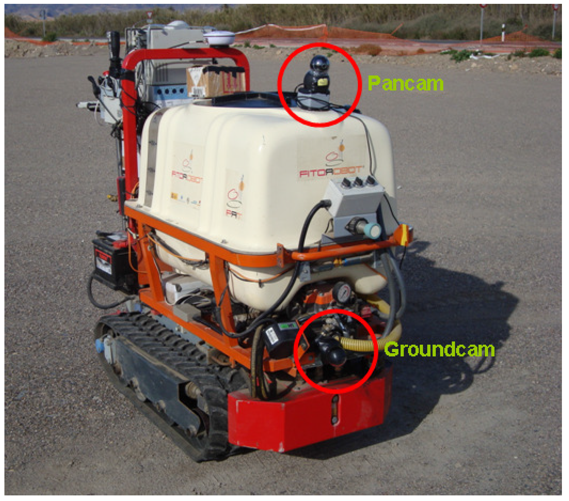
The mobile robot used as a testbed in this research consists of a rubber-track vehicle with differential steering (
Figure 2). This robot, called
Fitorobot, was developed by the University of Almería (Spain) for spraying purposes inside greenhouses [
1]. The motivation for using this robot is that it constitutes a known platform and it has shown its suitability as a research testbed in off-road conditions, mainly in planar and quasi-planar terrains [
1]. Previous physical experiments carried out with
Fitorobot in off-road conditions are discussed in [
1]. These experiments deal mainly with motion control, localization, and slip estimation.
The mobile robot Fitorobot is 0.7 (m) wide, 1.7 (m) long, and 1.5 (m) height. The weight of the vehicle is 500 (Kg). The robot may achieve a maximum velocity of 2 (m/s), and it can face a slope of up to 5 (deg). Regarding the locomotion system, the track radius is 0.15 (m), the track width is 0.18 (m), and the track length is 0.75 (m). Steering is accomplished by changing the velocities of two hydraulic gear motors, achieving turning radii of nearly zero.
Two units of one consumer-grade camera have been used, Logitech® 2 Mpixel QuickCam Sphere AF webcam with a maximum frame rate of 30 (fps). In this case, a spatial resolution of (px) has been chosen. The camera calibration has been obtained using the “Camera Calibration Toolbox for Matlab®”.
It bears mentioning that the position and height of the downward-looking camera has been carefully analyzed. In this case, the camera was mounted in front of the robot between both tracks at a height of 0.49 (m). This distance was obtained as a trade-off between shadow-reduction and classification performance. Notice that a higher distance leads to more features but shadows can appear. In contrast, a shorter distance corresponds to a smaller field of view where the probability of shadows in the images is reduced. However, this may lead to featureless images; see [
1] for more details.
3.2. Dataset
For our identification and classification experiments, we have collected many images in off-road terrains with the tracked mobile robot
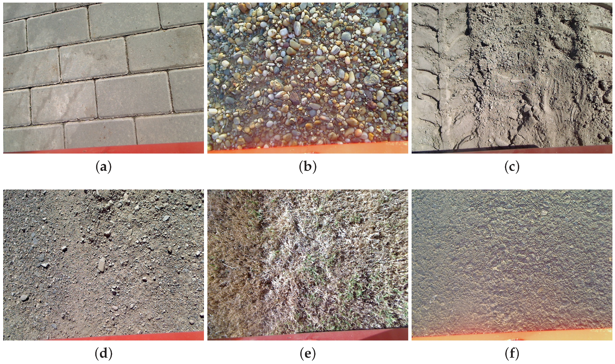
Fitorobot. There are seven major terrain types: pavement, gravel, grass, compact sand, sandy soil, asphalt, and wet pavement (see
Figure 3). Notice that these images cover typical environments in which an off-road mobile robot moves [
3]. For example, the robot might need to identify sandy terrains to avoid a high embedding risk, so that such terrain should be labeled as non-traversable by the motion planner. On the other hand, asphalt and gravel should be labeled as traversable, and hence, the robot should move primarily over them. We have included the wet pavement ground for comparison purposes, although there is a clear similarity with the pavement class. Nevertheless, we think it is useful to check the performance of our classification algorithms even using this class. Asphalt has also been included for comparison purposes. Notice that we have worked with different spatial resolutions depending on the classification algorithm. The images captured by the cameras have a resolution of
(px). The Gist-based classifier employs images with a resolution of
(px). This size was obtained as a trade-off between proper performance of the classification strategy and computation time. The color-based classifier works with
(px) rectified patches. Again, this size was obtained after analyzing the performance of the classifier. In particular, these rectified patches are obtained as subimages of the original frontal image. Thus, a larger dimension leads to featureless images because of perspective distortion, and smaller images mean a worse performance of the classifier.
In relation to the ground camera, we have collected a total of 1400 images (200 images for each of the seven classes). Regarding the frontal camera, we have collected several images for each class. These were then split using the rectification process explained subsequently, obtaining 74 images for each class. Specifically, we have used 2590 frontal patches in this research.
At this point, we would like to point out some issues related to the physical conditions in which these images were obtained. First of all, the robot mostly moved at a speed of 0.4–0.5 (m/s). The dataset includes a reasonable variety of surface conditions in each type of terrain. In particular, different grass sizes and differently-sized grains in the gravel terrain were considered. The images of the sandy terrain also present different traces. The rectangular bricks of the pavement surface were not always aligned in exactly the same orientation. Furthermore, special mention must be made of the fact that the images were taken on different days and at different hours, so different lighting conditions were ensured. When the robot moved close to 1 (m/s), we noticed a certain blur effect in the images. However, some of these images were retained in our dataset in order to check the robustness of our strategy.
4. Gist-Based Classifier for Ground Images
This section details the Gist-based classifier trained to identify the terrain beneath the robot. Before explaining the SVM classifier, which constitutes the core of this algorithm, the Gist descriptor is introduced.
4.1. Gist Descriptor
Traditionally in the field of computer vision, image signatures are employed for classification purposes. The overall image is represented by a vector of color components where a particular dimension of the vector corresponds to a certain subimage location [
20]. There are several ways to obtain an image signature [
20], although the most interesting solutions are based on determining global image descriptors.
The most typical ways to implement global descriptors are using textons [
21] and Gist [
22,
23]. Both descriptors are based on the same idea, that is, applying a bank of Gabor filters at various locations, scales, and orientations to a given image. A Gabor filter is a linear band-pass filter whose impulse response is defined as a Gaussian function modulated with a complex sinusoid [
24]. Depending on the frequency and the bandwidth terms used in such a function, a different filter is obtained.
Notice that a global descriptor based on textons has already been used in off-road mobile robots, see for example [
3,
25]. However, recent reports in the field of computer vision confirm that the Gist descriptor slightly outperforms textons [
26]. For this reason, we have considered the Gist descriptor in this research.
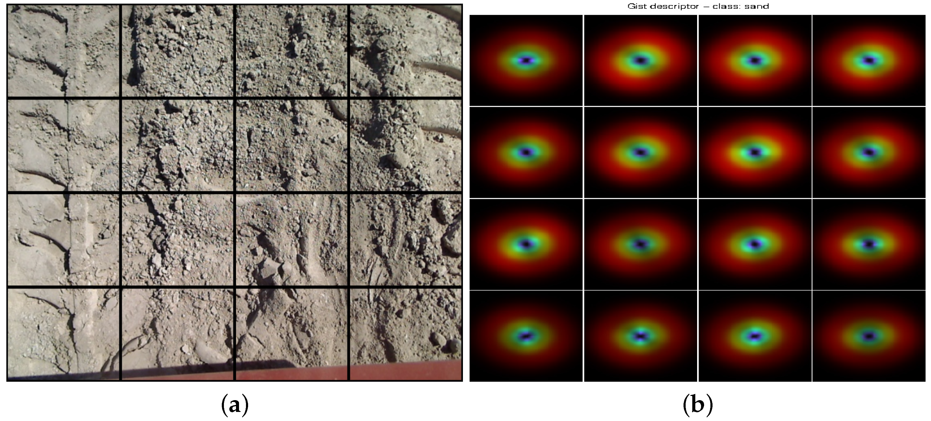
As already mentioned, the Gist descriptor is a global descriptor of an image that represents the dominant spatial structures of the scene captured in the image. In particular, the Gist descriptor computes the output energy of a bank of 24 filters. The filters are Gabor-like tuned to 8 orientations at 4 different scales. The square output of each filter is then averaged on a
grid.
Figure 4 shows the Gist-descriptor signature for sand. The Gist implementation that we have used first preprocesses the input image (ground image) by converting it to grayscale, then normalizes the intensities and scales the contrast. The image is split into a grid and a set of Gabor filters are applied to each cell. Finally, the average of these cells gives the Gist signature (vector of 512 values). In this research, we use the open-source Matlab
® implementation of the Gist descriptor available at [
22].
4.2. Support Vector Machine Classifier
Once the Gist descriptor has been introduced, the next step consists of implementing an image classifier. In this context, machine learning/classification techniques have been employed in various off-road mobile robotics applications, see for example [
27] and the references therein. In our case, we use the well-known Support Vector Machine (SVM) approach. Specifically, we provide a set of representative training images (represented by their Gist-descriptor signature) and their associated terrain (manually labeled). Then, the SVM classifier is trained offline. In query time, the trained SVM classifier is used to retrieve the terrain type in each image. The SVM feature space is 512 and the number of classes to be identified are seven (pavement, gravel, sand, compact sand, grass, asphalt, and wet pavement).
In order to increase the reliability of the results addressed in this research, we use the well-known 5-fold random cross-validation method for selecting the images used for training and testing the SVM [
28]. Additionally, different train/test splits have been considered (e.g., 10%–90%, 50%–50%).
The SVM classification is implemented using the open-source VLFeat library.
5. Color-Based Classifier for Frontal Images
This section describes the color-based classifier employed to classify frontal images. This is used because Gist+SVM does not work with frontal images (perspective distortion leads to featureless images). Therefore, the Gist signatures obtained are not sufficient to guarantee a proper classification with SVM. This poor performance is shown in
Section 7.1. As a first attempt to solve this issue we have used a well-know solution in computer vision, that is, color-based classification [
29,
30]. However, instead of using the RGB color space we have considered the HSV color space. This color space has been employed for three reasons: (i) it decouples the color-carrying information into one single color channel (i.e., Hue); it is easier to work with this vector only than with three vectors (R, G, B); (ii) HSV is less sensitive to varying lighting conditions (e.g., shadows) than other color spaces [
29]; (iii) HSV has demonstrated better performance in comparison with other color spaces in terms of image classification, see for example [
30].
Initially, original frontal images are split into smaller regions or subimages [
21]. After these regions are obtained from the frontal view, a rectification step is carried out in order to remove the perspective distortion. Finally, HSV color space is used to classify the images considering the histogram related to the Hue channel. In this research, we call these regions or subimages within a frontal image as patches (before removing the perspective distortion) and “rectified patches” once the rectification process has been applied.
Figure 5 shows the difference between a patch and a rectified patch.
5.1. Image Rectification
At this point, we explain the process followed in order to remove the perspective distortion effect by using a planar homography. It bears mentioning we are comparing each patch with a dataset of hand-labeled patches through a color-based classifier based on the nearest distance between the histograms (see
Section 5.2 and Step 3 in the proposed methodology in
Section 6). This dataset includes the patches labeled according to the true class (see Remark 1).
Remark 1. The histogram computed on the rectified patch is not the same than the histogram computed when the patch is not rectified. When the patch is rectified using the homography, the importance of all the areas of the patch is the same. Areas far from the camera, that due to the camera perspective receive less pixels in the frontal image, have, in the rectified patch, the same number of pixels than closer areas to the camera. This step is performed in order to obtain a more general solution independent of the perspective distortion. Additionally, it bears mentioning non-rectangular patches would be troublesome because current computer vision libraries work mostly with squared/rectangular images.
Mathematically, the rectification problem is formulated as [
31]
where
is a projection matrix (
g refers to the ground camera and
f to the frontal camera),
I is the identity matrix,
are the upper triangular camera calibration matrices dealing with intrinsic parameters (focal lengths and principal points),
R is a rotation matrix and
is a translation vector. The ground plane is
. Then, the homography,
H, induced by the ground plane is given by [
31]
Considering Equation (
2), the image rectification to be applied is given by
where
are the points on the ground plane and the frontal plane (pixel units), respectively. In this case,
with
. Notice that
R represents an Euclidean clockwise rotation about the
x -axis (see
Figure 2b).
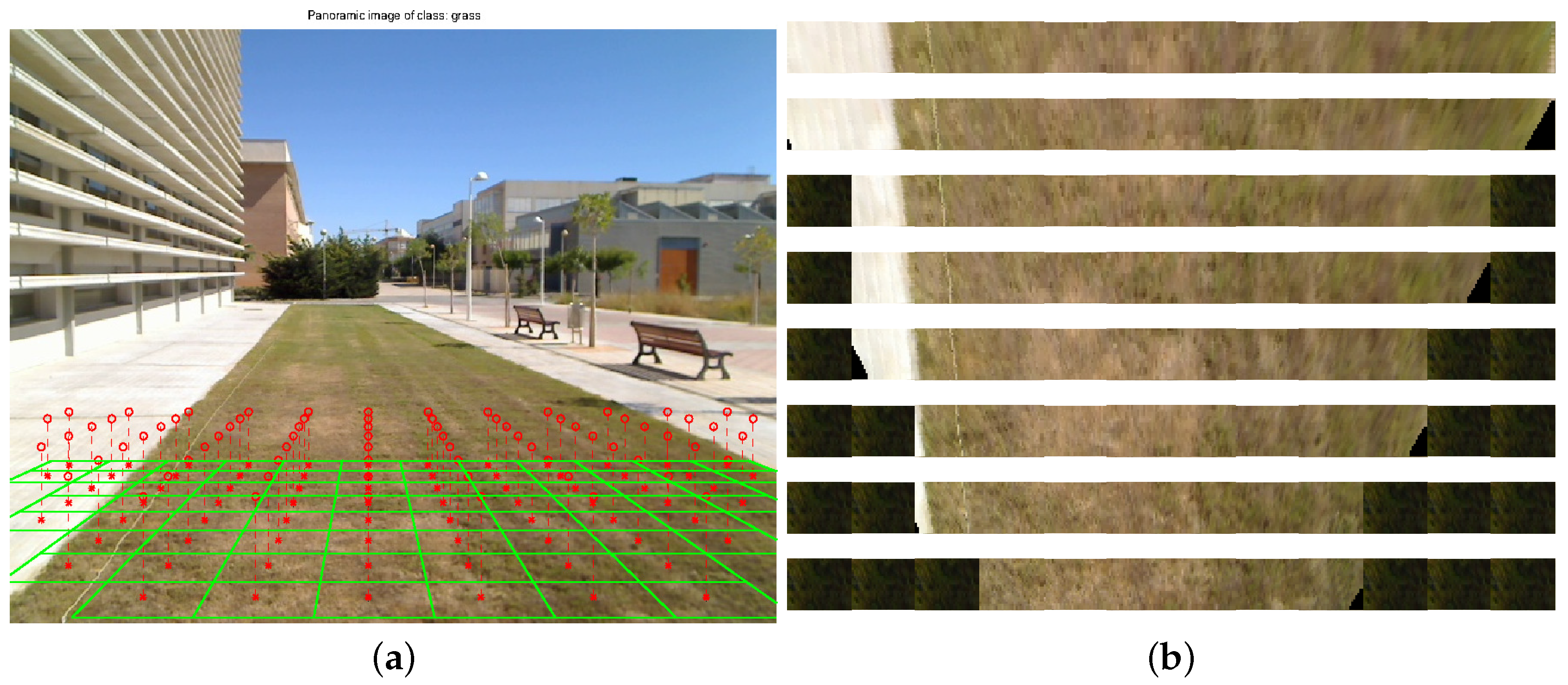
Figure 5 shows the process of image rectification considering one frontal image (grass). The mesh considered for splitting the original image has been established as a trade-off between distance from the robot and the number of features of the patch obtained. It bears mentioning that further distance benefits path planning but leads to patches with few features and, hence, misclassification increases.
5.2. Classification Based on Histogram Intersection
Once the rectified patches have been extracted from the frontal images and converted to the HSV color model, we apply a color-based classifier based on the nearest distance between the histogram of the current patch and a set of representative rectified patches stored in a database (currently 74 patches/class). The result of the classifier is obtained as the mode of the ten closest rectified patches (the smallest distances between the histograms). The image histogram consists of a 256-dimensional vector representing the frequency of occurrence of each hue value. It is important to point out that we evaluated different metrics to compare the histograms: Euclidean distance, Kolmogorov-Smirnov distance, and statistics. The best result (the highest success rate) was obtained with statistics, and for this reason it was considered in this research.
Regarding implementation issues, we have used the open-source Histogram-distances Matlab
® toolbox [
32].
6. Complete Classifier Combining Ground and Frontal Images
In this section we detail the procedure carried out in order to increase the confidence in the classification of a given rectified patch. The prior color-based classification is combined with the identification of the terrain beneath the robot. Recall that this identification is the result of the Gist-based classifier applied to ground images. The procedure is summarized as follows:
Convert the current rectified patch to HSV color space. From now on the rectified patch in the HSV color space is denoted as p.
Obtain the histogram related to the Hue channel. In mathematical terms
where
ω is the histogram of the Hue channel.
Calculate the distance between the current rectified patch and the hand-labeled database of histograms based on
statistics (recall
Section 5.2). Notice that the set of histograms is represented by Ω and its associated classes as Σ. Then, we can write
where Ψ is the vector with the distances and
is a function that calculates the distance between the vector
a and each row of the matrix
A in terms of
statistics.
Sort this vector of distances (from nearest elements to less similar values), that is,
where
is a vector of sorted distances, and
is the sorting function (min distance to max distance).
The class of the current rectified patch is obtained as the mode of the first ten values of the vector of distances (we have considered 10 values based on empirical tests)
where
α is the mode of the first ten elements of the vector
, and
is the class of the terrain identified through the color-based classification.
At this point, we intend to improve the classification
using the classification of the terrain beneath the robot,
(recall
Section 4). We refer to this new class as
. First we determine the following vector
where Υ is the new vector of distances between the histogram of the current rectified patch and the set of hand-labeled histograms, Ω. Notice that the correction coefficient,
, is only applied to the elements of
that have been classified with the same class as the ground image. The parameter
is determined in terms of the distance between the robot and the rectified patch, that is,
where the variable
is a parameter that represents the confidence of the color-based classifier. From experimental evidence,
. Notice that these values are in fact the accuracy of each terrain class while considering the color-based classifier (see
Figure 8). The function
gives a value depending on the distance between the position of the rectified patch and the robot. This distance is obtained using the calibration parameters of the frontal camera.
The parameters γ and η were experimentally tuned for each particular class, that is, the weighting coefficient depends on the class identified by the Gist-based classifier. More specifically, the parameters were obtained after a trade-off because a larger value might lead to misclassification in heterogeneous environments. Imagine an environment where the robot is on compact sand only (detected by the Gist-based classifier), but the frontal images comprise several environments, which are detected by the color-based classifier. If δ applies a large correction value, the patches belonging to a different class from compact sand might be misclassified as compact sand, even though the color-based classifier was functioning correctly. After empirical analysis, γ and η have been tuned in a way that δ is within the range {0.75, 0.9} in order to avoid the misclassification effect previously explained.
The practical meaning of Equation (
5) is that it is a function that decreases the difference between the histogram of the current rectified patch and those rectified patches that have the same class as the gist-based classifier (ground images). This coefficient is smaller (larger correction) when the rectified patches are closer to the robot (distance function), but it becomes larger (lower correction) when the patches are further from the robot. This means that the confidence in the ground-based classification decreases with distance. This represents a valid assumption because the further away the patch, the lower is the possibility that such terrain immediately beneath the robot.
Sort again the vector of distances
where
is the new vector of distances taking into account the correction offered by the downward-looking camera.
Finally, the new class is obtained as the mode of the first ten values of the vector of distances, that is,
This procedure leads to a reduction in the misclassification of the terrain in the frontal images because: (1) the classification of the terrain beneath the robot is almost perfect due to the finer resolution of the images and the high performance of the Gist+SVM classifier (success classification rate > 96.5%); (2) the preliminary color-based classification is updated taking into account the correction factor applied at step 6. It is also important to remark that in order to increase the performance, a 7-neighbor filter has been implemented. Specifically, we compare the class of the current rectified patch with the classes of its 7 neighbors (upper patch, upper right and upper left patches, right and left patches, lower right and left patches). If the classes of the 7 neighbors (4 to the right and 4 to the left) are the same, but do not match that of the current rectified patch, the class of this patch is updated to the class of its neighbors.
7. Experiments
This section, dealing with physical experiments, it is divided into two parts. The first part compares results using the Gist-based classifier, the color-based classifier, and the combination of both classifiers. Real images of the different terrain types are employed for this purpose. The confusion matrix is displayed in order to analyze the performance of each classifier. Recall that, the confusion matrix shows what percentage of the test examples belonging to a class have been classified as belonging to any of the seven available classes. Its diagonal shows the correct classification rate for each class and the off-diagonal elements show how often one class is confused with another [
3].
It bears mentioning that we use the 5-fold random cross-validation method for selecting the images used for training and testing the SVM. Furthermore, different train/test splits demonstrate the performance of the Gist-based classifier.
The second part of this section evaluates the performance of the color-based classifier and the classifier based on combining ground and frontal images. In this case, three outdoor environments are considered. The first two scenarios mix two different terrain types. The third consists of one single terrain type but with a significant shadow appearing in the image.
7.1. Gist-Based Classifier
The first step in our research was to investigate the performance of the Gist-based classifier in terms of the resolution of the image. We considered 110 images for each class resulting in 770 images. In this case, 50% of the images were randomly selected for training the SVM classifier and 50% were used for testing. The metrics employed for analyzing the performance of the Gist-based classifier deals with the number of images successfully classified in their true class and the time employed for the simulation.
Table 1 summarizes the performance of each patch size and the computation time required to proceed each single patch. Recall that, this analysis has been run on a processor 2.9 GHz Intel Core i7, 8 GB RAM and with Matlab R2014b.
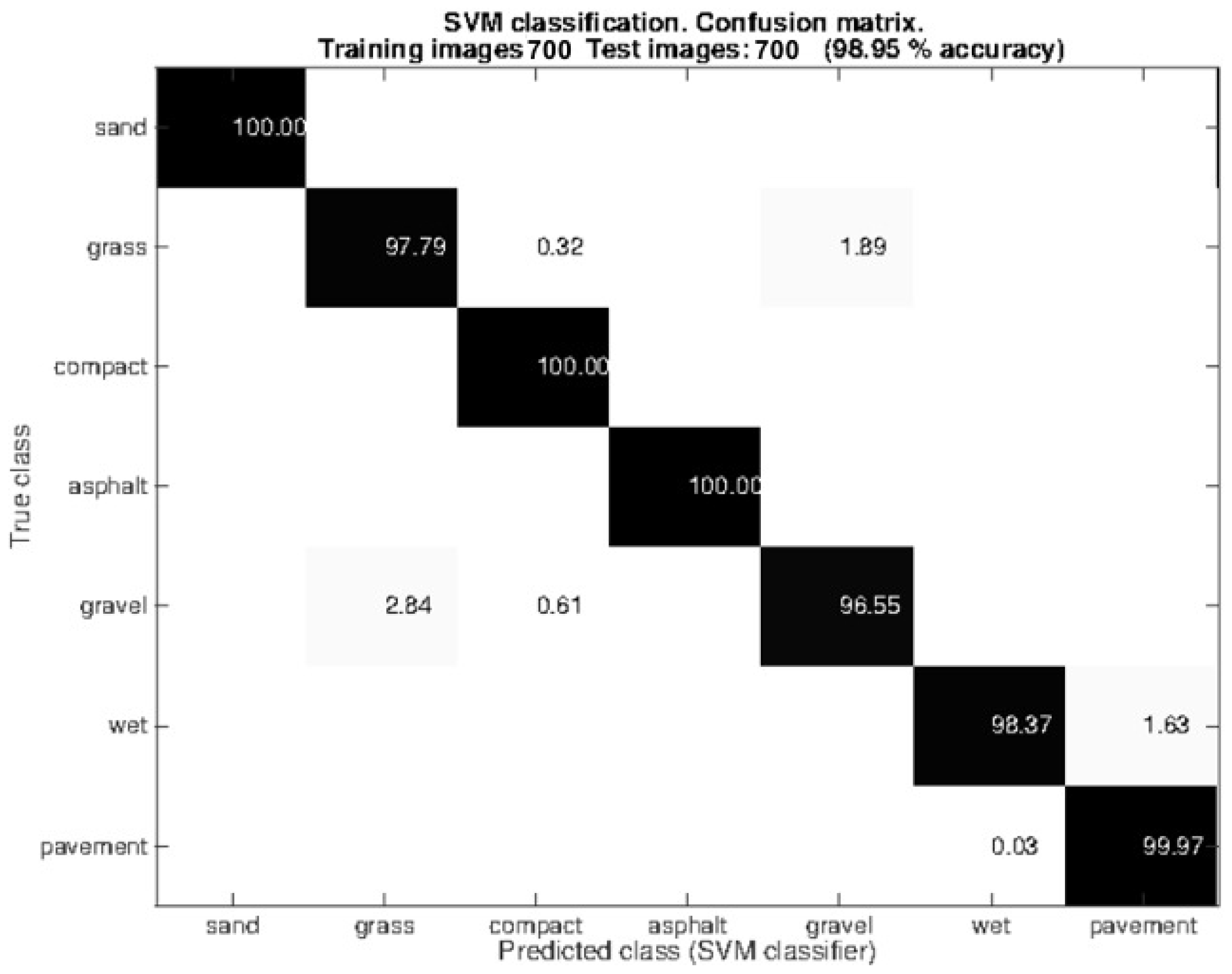
After this analysis, the size
(px) was selected for comparing the images during the query time as a compromise between performance and computation time. As explained, the 5-fold random cross-validation approach was used for splitting the dataset. After that, 50% of the images were used for training the SVM and 50 % for testing it. Furthermore, we have added 90 images more for each class. This resulted in a dataset of 1400 images (
), 700 used for training the SVM and 700 for testing it.
Figure 6 shows the confusion matrix related to the testing images. Observe that the Gist + SVM classifier operates correctly with almost all the classes. Grass is sometimes misclassified with compact sand (0.32%) and gravel (1.89%), which can be explained by the fact that the grass in certain regions was very short and closely resembles compact sand or gravel. Gravel is also misclassified with grass (2.84%) and compact sand (0.61%). Again, this result shows the similarity between these classes. It is not surprising that the wet pavement and dry pavement are sometimes misclassified given that in certain images the amount of water in the wet pavement is small.
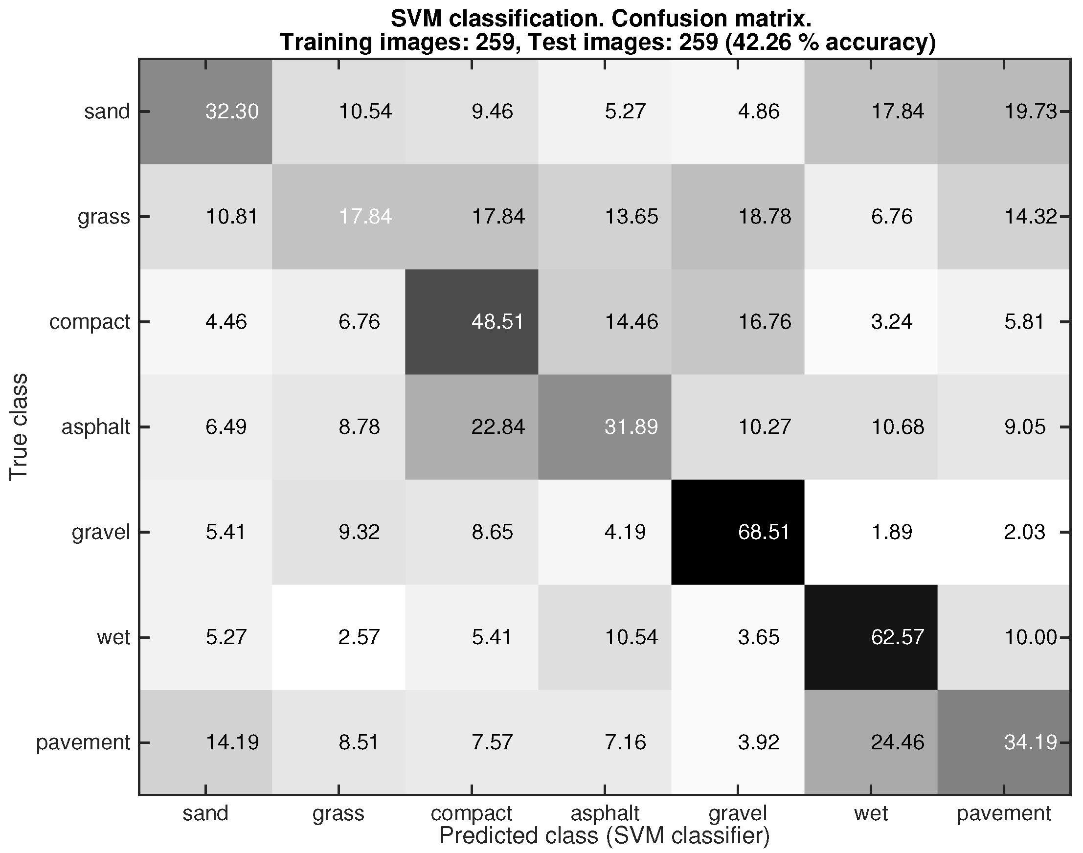
After analyzing the performance of the Gist-based classifier with the ground images, we tested this classifier with the rectified patches obtained from the frontal view, see
Figure 7. In this experiment 518 rectified patches were employed (
). Again the 5-fold random cross-validation approach was used for splitting the dataset. After that, 50% of the rectified patches were used for training and the other 50% for testing. As can be seen the overall performance of the Gist-based classifier was fairly poor (42.26%). For instance, only 17.84% of the images labeled as grass were properly classified. The best classification was achieved with gravel, but only 68.51% of the rectified patches were properly classified. This result led to the decision to use the color-based classifier for dealing with the frontal images.
7.2. Color-Based Classifier
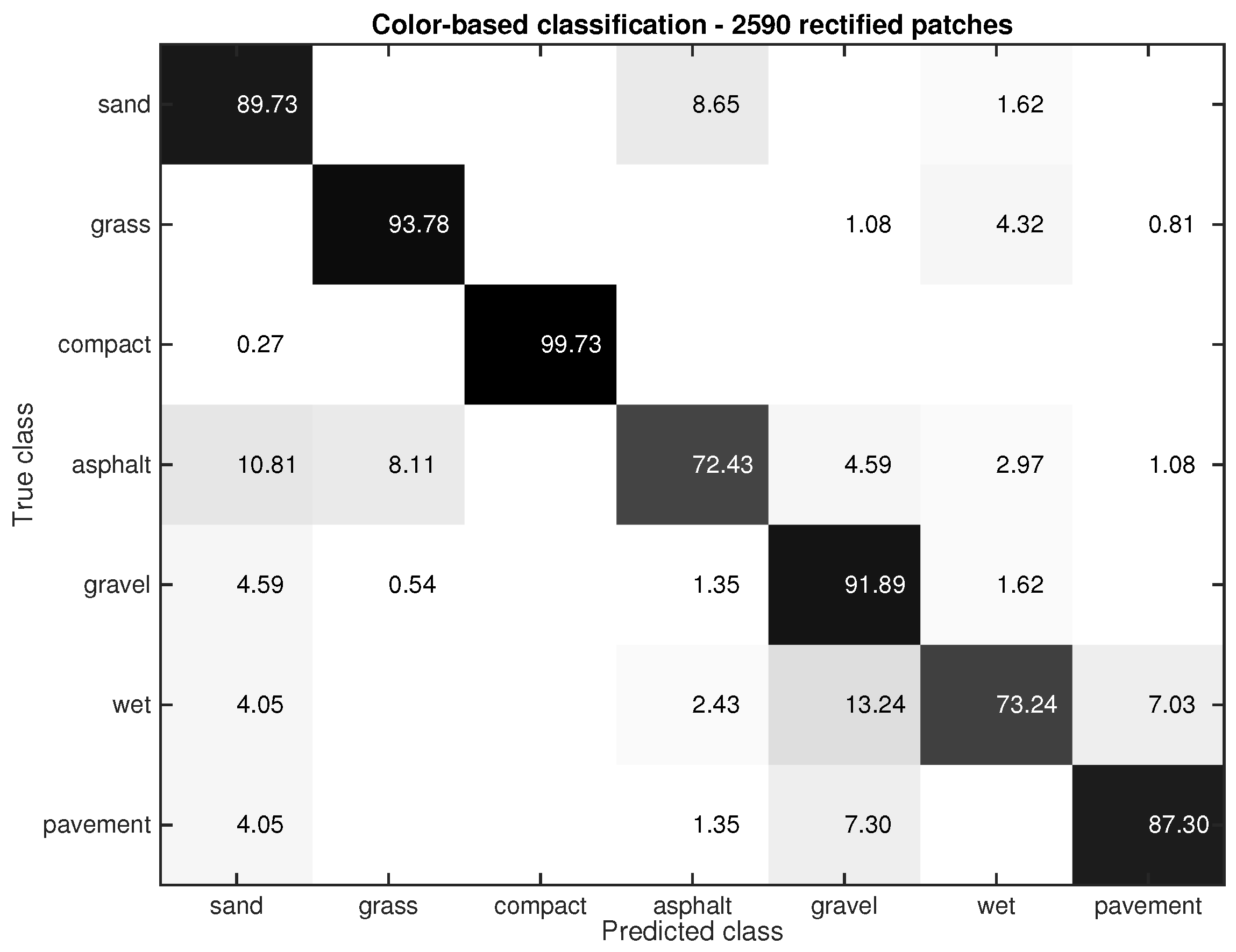
Two different resolutions were tested for the rectified patches extracted from the frontal image,
(px) and
(px). The smaller size gave a slightly better result than the larger size. The performance of the color-based classifier using rectified patches of
(px), is shown in
Figure 8. Five representative images of the 7 terrain types were used. Seventy four rectified patches were then extracted from each class leading to a total of 2590 rectified patches. The confusion matrix shows the mean value of the classification rate. It can be seen why color-based classification is preferred over Gist-based classification. Notice that with the color-based classifier every class is correctly classified with an accuracy greater than 72%. The worst classification is achieved for asphalt and wet pavement (72.43%, 73.24%).
7.3. Complete Classifier Combining Ground and Frontal Images
In this section, we also use the dataset employed in the previous section (2590 rectified patches). We take into account the information provided by the Gist-based classifier to improve the former color-based classification, i.e., we use the information from the downward-looking camera.
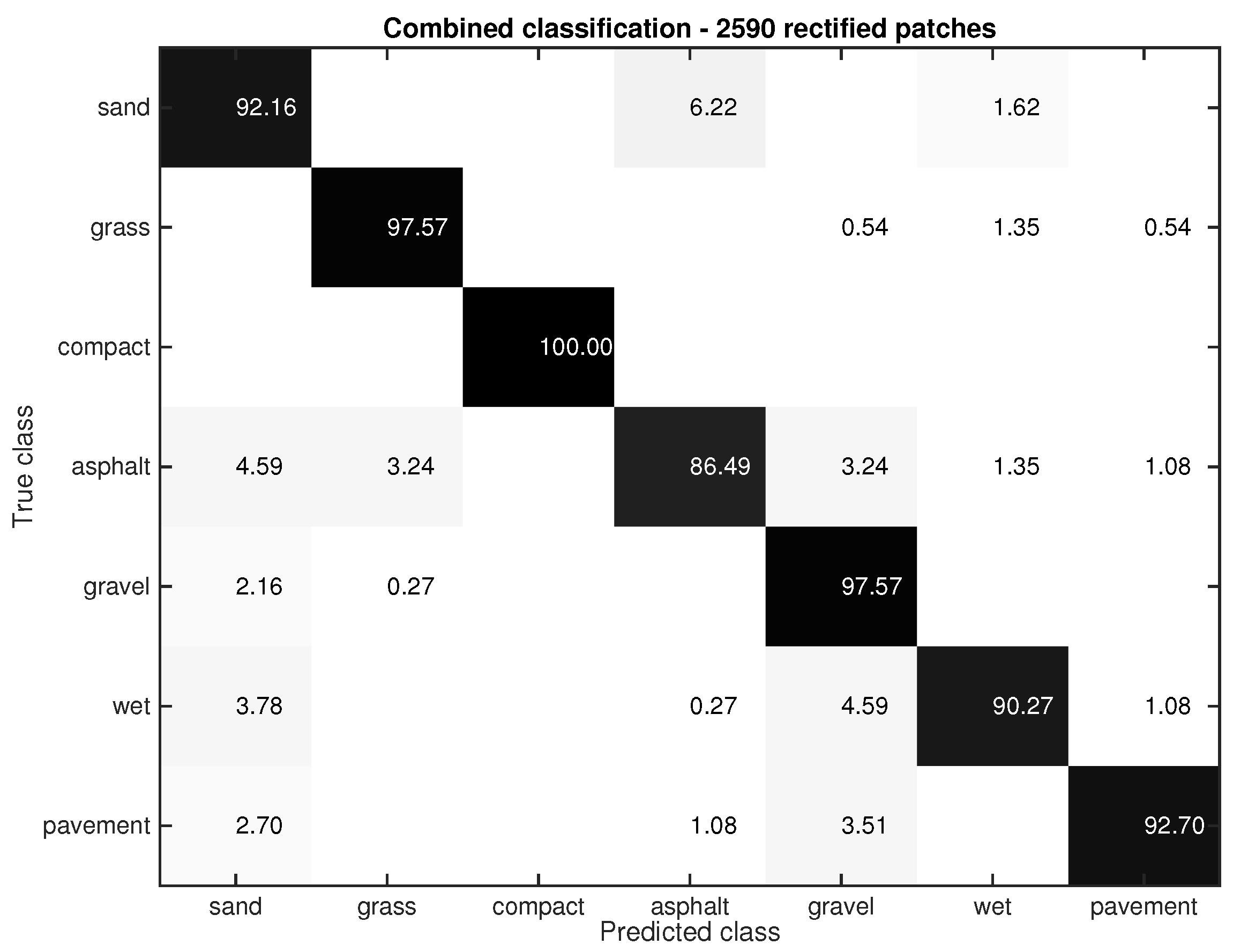
Figure 9 shows the confusion matrix. Notice that the classification success increases significantly (93.83 versus 86.87). For example, the success rates of asphalt and wet pavement are: 86.49% and 90.27% versus the 72.43% and 73.24% achieved with the color-based classifier. This improvement is also noticeable in sand (92.16% versus 89.73%), grass (97.57 % versus 93.78%), compact sand (100% versus 99.73%), gravel (97.57% versus 91.89%), and pavement (92.70% versus 87.30%). Observe that the success rate increases around 15% in the asphalt and wet classes, that is, the classes with the worst performance in the color-based classifier (see
Figure 8). This result does reinforce the contribution of this paper, that is, combining frontal and ground images not only improves the classification (∼5%), but this improvement is even bigger in the most challenging classes (i.e., asphalt and wet).
7.4. Proposed Framework for Terrain Classification
In this section, we compare the performance of the proposed classifier with the color-based classifier in three different scenarios.
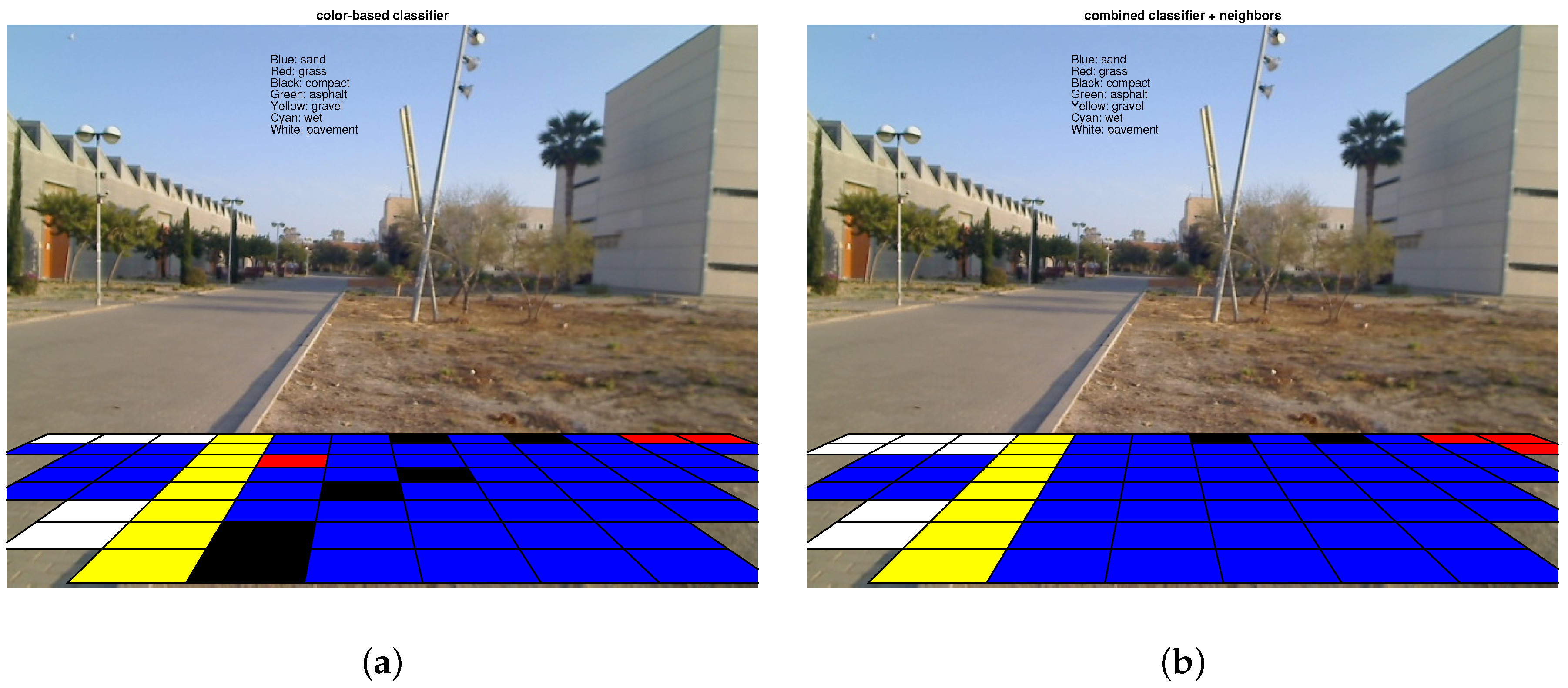
Figure 10 shows results from the first experiment. In this case, sandy soil and pavement are present in the frontal view; the robot is on sandy terrain. This experiment shows the poor performance of the color-based classifier because several patches are misclassified as compact sand (black cells) and as grass (red cells). Furthermore, some patches relating to the pavement are misclassified as sand. The rectified patches dealing with the curbstone do not belong to any particular class, although here they are classified as gravel. This does not represent misclassification because this class (curbstone) was not considered in this research. Observe that the complete classifier improves the former result. In particular, now only 4 patches are misclassified as opposed to 9 misclassified by the color-based classifier (sandy area). Notice that although the robot is actually on sandy terrain, the proposed classifier with the 7-neighbor filter also improves the classification of the patches on pavement (6 patches versus 9 patches by the color-based approach). The complete classifier achieves a misclassification rate of 10% as against the 24.32% of the color-based classifier.
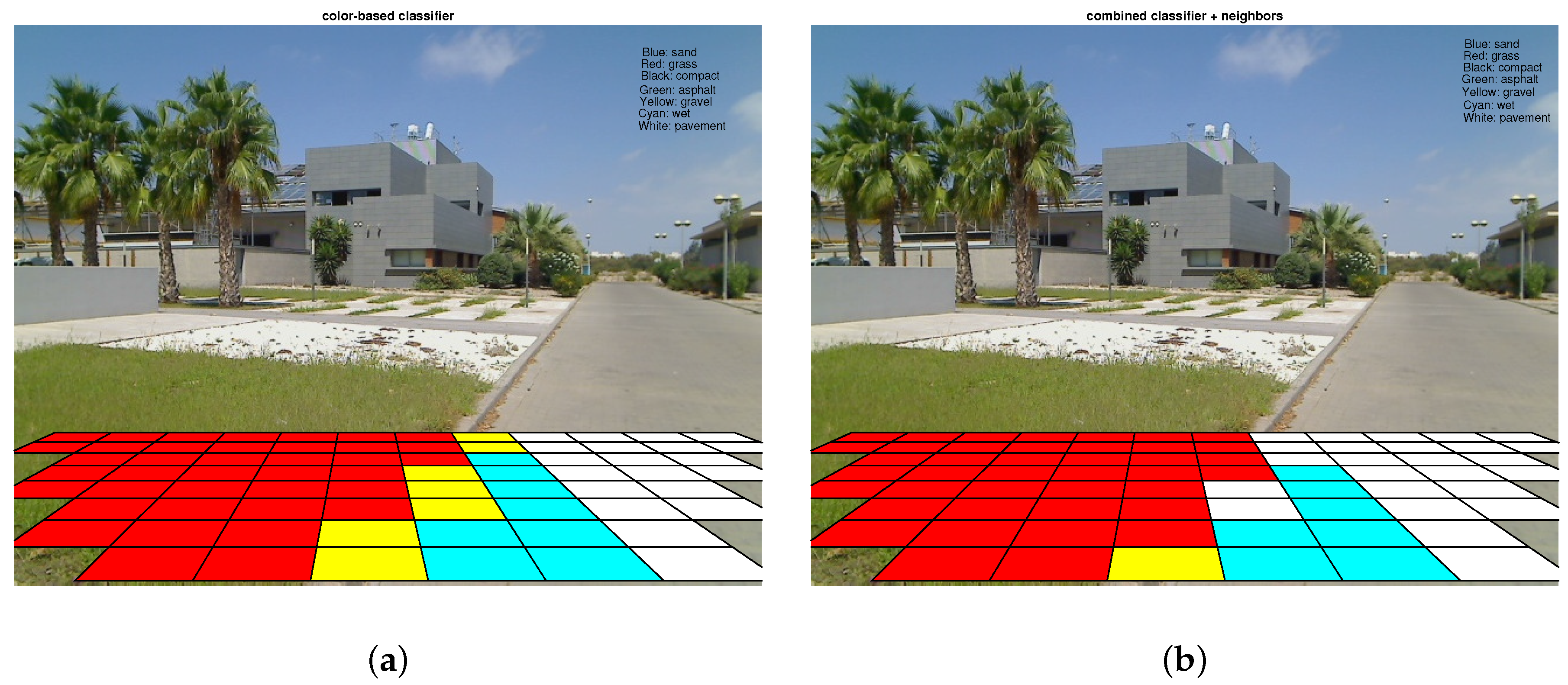
Figure 11 details the second physical experiment. In this case, two classes are found in the original frontal image: grass and pavement. The robot was moving on pavement. Several conclusions can be extracted from this experiment. First, the grass is perfectly identified. Secondly, notice that some rectified patches are misclassified as wet pavement. This is not altogether unexpected because, as previously mentioned, depending on the lighting conditions wet pavement and dry pavement are very similar. In any case, the improved performance of the classifier combining ground and frontal images (complete classifier) is demonstrated. In particular, the color-based classifier (considering only frontal images) misclassifies 15 rectified patches, while the combined classifier misclassifies only 8 patches. In conclusion, the complete classifier achieves a misclassification rate of 10.81% as against the 20.27% of the color-based classifier.
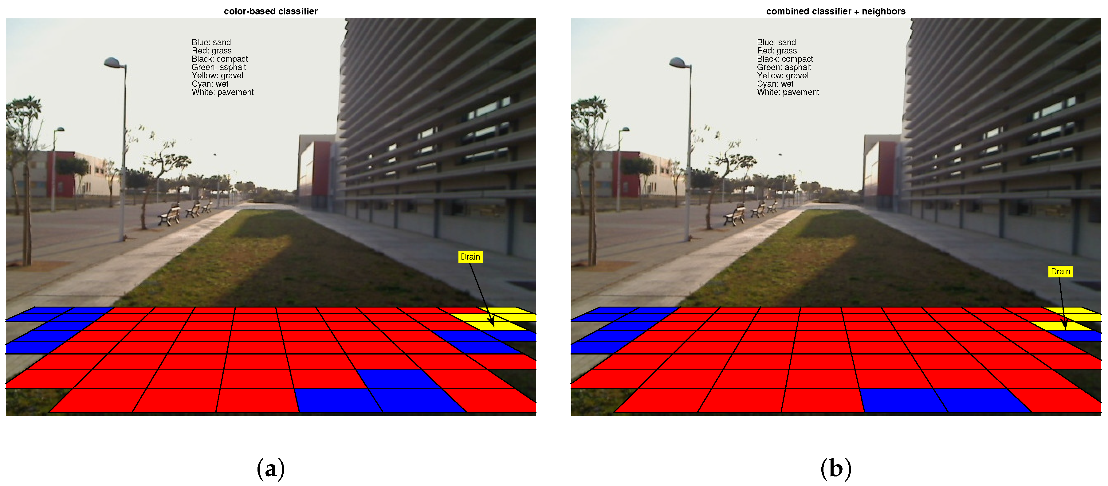
One last experiment shows the performance of the color-based classifier and the improvement obtained by means of the complete classifier. In this case, a frontal image with a hard shadow is considered, see
Figure 12. Now only one class is present, grass, although an “unknown” type of terrain (concrete floor) appears on the left side of the image and another “unknown” terrain (a drain) appears in the middle. Recall that in outdoor scenarios the lighting is uncontrolled and may lead to misclassification, as remarked in [
3,
15]. This experiment shows an appropriate performance of the combined classifier. Despite the presence of shadows, the misclassification rate of this classifier is 8.62%. The color-based classifier has a misclassification rate of 15.51%.
These results demonstrate the main contribution of this paper, that is, combining ground-view information with frontal-view information improves the performance in the classification of the rectified patches extracted from the frontal images. Now, if the robot had to move in an environment such as that identified in
Figure 11, for example, the path planner would have selected moving on pavement as much as possible. Notice that trafficability is much better on pavement than on grass terrain and, hence, the risk of entrapment is much smaller in pavement [
1].
8. Conclusions
This paper presents a novel terrain classification strategy by which information obtained from a downward-looking camera and a frontal camera is combined in order to improve the identification of the forthcoming terrain. Several experiments show the improvement achieved by combining information about the ground beneath the robot with frontal information using the complete classifier compared to using a typical color-based classifier which only takes frontal information into account. For example, in the experiment using 2590 rectified patches (
Section 7.3) the classification rate achieved by the complete classifier is 93.83% as compared to 86.87% achieved with the color-based classifier. Additionally, three challenging experiments in mixed scenarios show that the misclassification rate of the complete classifier is almost half that given by the color-based classifier (10% vs. 24.32%; 10.81% vs. 20.27%; 8.62% vs. 15.51%). These results provide evidence of the good performance of the suggested approach despite the fact that the terrains used for testing the classifiers were different from those used for creating the dataset and those employed for training the learning algorithm. This fact demonstrates the robustness of our approach, especially in terms of shadows, and different conditions in the terrains. Future efforts will focus on testing in more challenging terrains (uneven terrains) adding a telecentric lens.
This paper also contributes a comparison between the performance of the Gist-based classifier and the computational cost. In particular, the best performance is obtained when the size of the image is 640 × 480 (px), however, it leads to the greater computation time (1.3 (s) per image). The best trade-off is obtained for the size 160 × 120 (px), which means a performance similar to the previous case but it only requires 0.18 (s) per image.
This research constitutes the first application of the Gist descriptor to mobile robotics. Our main motivation for using it here was that: (i) it outperforms the known texton-based descriptors; and (ii) for classification purposes (SVM classifier) it is convenient to constrain the information appearing on an RGB image to one single vector (global descriptor). In this case, the Gist signature of an image reduces spatial structures of the scene to a 512-dimensional vector.
This paper has also demonstrated how two low-cost cameras can be successfully used to predict the forthcoming terrain in off-road conditions (Logitech® 2 Mpixel QuickCam Sphere AF webcam, <300€). However, it is expected that better cameras will lead to an improvement in the results discussed here. This issue is also part of future research. Additionally, notice that omnidirectional cameras will be welcome because omnidirectional vision adds more information to the mobility map and hence a better path might be selected to reach a given goal (not only considering the forward direction, as now).
Future research will include an exhaustive testing of the mobile robot in different terrains in order to estimate more properties of such terrains (e.g., slip, sinkage, cohesion, internal friction angle). It is also important to point out that visual information alone might not be sufficient to distinguish various terrain types in a broad sense. For this reason, the next research step will deal with combining information from other sources like multispectral imaging. The integration of the proposed approach within a closed-loop navigation architecture will be addressed in the coming research.
Acknowledgments
The authors thank the University of Almeria, in particular J. Sánchez-Hermosilla and F. Rodríguez, for giving us access to the tracked mobile robot Fitorobot. This work is framed within the Project DPI2015-65962-R (MINECO/FEDER, UE).
Author Contributions
R. Gonzalez and A. Rituerto conceived the algorithms and performed the experiments; R. Gonzalez, A. Rituerto and J.J. Guerrero analyzed the data; R. Gonzalez wrote the paper.
Conflicts of Interest
The authors declare no conflict of interest. The founding sponsors had no role in the design of the study; in the collection, analyses, or interpretation of data; in the writing of the manuscript, and in the decision to publish the results.
References
- Gonzalez, R.; Rodriguez, F.; Guzman, J.L. Autonomous Tracked Robots in Planar Off-Road Conditions. Modelling, Localization and Motion Control; Series: Studies in Systems, Decision and Control; Springer: Berlin/Heidelberg, Germany, 2014. [Google Scholar]
- Wong, J. Theory of Ground Vehicles, 3rd ed.; John Wiley & Sons, Inc.: Hoboken, NJ, USA, 2001; p. 528. [Google Scholar]
- Angelova, A.; Matthies, L.; Helmick, D.; Perona, P. Learning and Prediction of Slip from Visual Information. J. Field Robot. 2007, 24, 205–231. [Google Scholar] [CrossRef]
- Wong, J. Terramechanics and Off-Road Vehicle Engineering, 2nd ed.; Butterworth-Heinemann (Elsevier): Oxford, UK, 2010. [Google Scholar]
- Iagnemma, K.; Kang, S.; Shibly, H.; Dubowsky, S. Online Terrain Parameter Estimation for Wheeled Mobile Robots with Application to Planetary Rovers. IEEE Trans. Robot. 2004, 20, 921–927. [Google Scholar] [CrossRef]
- Ojeda, L.; Borenstein, J.; Witus, G.; Karlsen, R. Terrain Characterization and Classification with a Mobile Robot. J. Field Robot. 2006, 23, 103–122. [Google Scholar] [CrossRef]
- Ray, L.E. Estimation of Terrain Forces and Parameters for Rigid-Wheeled Vehicles. IEEE Trans. Robot. 2009, 25, 717–726. [Google Scholar] [CrossRef]
- Brooks, C.; Iagnemma, K. Vibration-based Terrain Classification for Planetary Exploration Rovers. IEEE Trans. Robot. 2005, 21, 1185–1191. [Google Scholar] [CrossRef]
- Libby, J.; Stentz, A. Using Sound to Classify Vehicle-Terrain Interactions in Outdoor Environments. In Proceedings of the IEEE International Conference on Robotics and Automation (ICRA), Stockholm, Sweden, 16–21 May 2016; IEEE: Saint Paul, MN, USA, 2012; pp. 3559–3566. [Google Scholar]
- Bellutta, P.; Manduchi, R.; Matthies, L.; Owens, K.; Rankin, A. Terrain Perception for DEMO III. In Proceedings of the IEEE Intelligent Vehicles Symposium, Dearborn, MI, USA, 3–5 October 2000; pp. 326–331.
- Manduchi, R.; Castano, A.; Talukder, A.; Matthies, L. Obstacle Detection and Terrain Classification for Autonomous Off-Road Navigation. Auton. Robot. 2005, 18, 81–102. [Google Scholar] [CrossRef]
- Helmick, D.; Angelova, A.; Matthies, L. Terrain Adaptive Navigation for Planetary Rovers. J. Field Robot. 2009, 26, 391–410. [Google Scholar] [CrossRef]
- Bajracharya, M.; Howard, A.; Matthies, L.; Tang, B.; Turmon, M. Autonomous Off-Road Navigation with End-to-End Learning for the LAGR Program. J. Field Robot. 2009, 26, 3–25. [Google Scholar] [CrossRef]
- Dille, M.; Grocholsky, B.; Singh, S. Outdoor Downward-facing Optical Flow Odometry with Commodity Sensors. In Field and Service Robotics; Springer: Berlin, Germany, 2010; pp. 183–193. [Google Scholar]
- Nourani-Vatani, N.; Borges, P. Correlation-Based Visual Odometry for Ground Vehicles. J. Field Robot. 2011, 28, 742–768. [Google Scholar] [CrossRef]
- Song, X.; Althoefer, K.; Seneviratne, L. A Robust Downward-Looking Camera Based Velocity Estimation with Height Compensation for Mobile Robots. In Proceedings of the International Conference Control, Automation, Robotics and Vision, Singapore, 7–10 December 2010; pp. 378–383.
- Ishigami, G.; Nagatani, K.; Yoshida, K. Slope Traversal Controls for Planetary Exploration Rover on Sandy Terrain. J. Field Robot. 2009, 26, 264–286. [Google Scholar] [CrossRef]
- Nagatani, K.; Ikeda, A.; Ishigami, G.; Yoshida, K.; Nagai, I. Development of a Visual Odometry System for a Wheeled Robot on Loose Soil using a Telecentric Camera. Adv. Robot. 2010, 24, 1149–1167. [Google Scholar] [CrossRef]
- Reina, G.; Ishigami, G.; Nagatani, K.; Yoshida, K. Odometry Correction using Visual Slip Angle Estimation for Planetary Exploration Rovers. Adv. Robot. 2010, 24, 359–385. [Google Scholar] [CrossRef]
- Datta, R.; Joshi, D.; Li, J.; Wang, J. Image Retrieval: Ideas, Influences, and Trends of the New Age. ACM Comput. Surv. 2008, 40, 1–60. [Google Scholar] [CrossRef]
- Leung, T.; Malik, J. Representing and Recognizing the Visual Appearance of Materials using Three-Dimensional Textons. Int. J. Comput. Vis. 2001, 43, 29–44. [Google Scholar] [CrossRef]
- Oliva, A.; Torralba, A. Modeling the Shape of the Scene: A Holistic Representation of the Spatial Envelope. Int. J. Comput. Vis. 2001, 42, 145–175. [Google Scholar] [CrossRef]
- Murillo, A.; Singh, G.; Kosecka, J.; Guerrero, J. Localization in Urban Environments using a Panoramic Gist Descriptor. IEEE Trans. Robot. 2013, 29, 146–160. [Google Scholar] [CrossRef]
- Risojevic, V.; Momic, S.; Babic, Z. Gabor Descriptors for Aerial Image Classification. In Adaptive and Natural Computing Algorithms; Lecture Notes in Computer Science; Dobnikar, A., Lotric, U., Ster, B., Eds.; Springer: Berlin/Heidelberg, Germany, 2011; Volume 6594, pp. 51–60. [Google Scholar]
- Martinez-Gomez, J.; Fernandez-Cabellero, A.; Garcia-Varea, I.; Rodriguez, L.; Romero-Gonzalez, C. A Taxonomy of Vision Systems for Ground Mobile Robots. Int. J. Adv. Robot. Syst. 2014, 11, 1–26. [Google Scholar] [CrossRef]
- Xiao, J.; Hays, J.; Ehinger, K.; Oliva, A.; Torralba, A. SUN Database: Large Scale Scene Recognition from Abbey to Zoo. In Proceedings of the IEEE Conference on Computer Vision and Pattern Recognition, San Francisco, CA, USA, 13–18 June 2010; IEEE Computer Society: Washington, DC, USA, 2010; pp. 3485–3492. [Google Scholar]
- Albus, J.; Bostelman, R.; Chang, T.; Hong, T.; Shackleford, W.; Shneier, M. Learning in a Hierarchical Control System: 4D/RCS in the DARPA LAGR Program. J. Field Robot. 2007, 23, 975–1003. [Google Scholar] [CrossRef]
- Arlot, S. A Survey of Cross-Validation Procedures for Model Selection. Stat. Surv. 2010, 4, 40–79. [Google Scholar] [CrossRef]
- Gonzalez, R.; Woods, R. Digital Image Processing, 3rd ed.; Prentice Hall: Upper Saddle River, NJ, USA, 2007. [Google Scholar]
- Kumar, J.; Gupta, N.; Sharma, N.; Rawat, P. A Review of Content Based Image Classification using Color Clustering Technique Approach. Int. J. Emerg. Technol. Adv. Eng. 2013, 3, 922–926. [Google Scholar]
- Hartley, R.; Zisserman, A. Multiple View Geometry in Computer Vision, 2nd ed.; Cambridge University Press: Cambridge, UK, 2003. [Google Scholar]
- Schauerte, B. Histogram Distances Toolbox. Available online: http://schauerte.me/code.html (accessed on 20 August 2015).
Figure 1.
General framework for terrain classification and characterization. Notice that the last step adds information about the particular properties of the terrain previously classified; in particular, information dealing with slip and sinkage.
Figure 1.
General framework for terrain classification and characterization. Notice that the last step adds information about the particular properties of the terrain previously classified; in particular, information dealing with slip and sinkage.
Figure 2.
Position of the cameras on the tracked mobile robot used as a testbed in this research.
Figure 2.
Position of the cameras on the tracked mobile robot used as a testbed in this research.
Figure 3.
Example images representing six of the terrain classes used in this research. Notice that these images have been taken by the downward-looking camera from 0.49 (m) above the ground. (a) Pavement; (b) Gravel; (c) Sand; (d) Compact sand; (e) Grass; (f) Asphalt.
Figure 3.
Example images representing six of the terrain classes used in this research. Notice that these images have been taken by the downward-looking camera from 0.49 (m) above the ground. (a) Pavement; (b) Gravel; (c) Sand; (d) Compact sand; (e) Grass; (f) Asphalt.
Figure 4.
Average filter energy in each bin. Notice that the standard Gist implementation considers 16 bins, 8 orientations, and 4 different scales, which explains why the Gist-descriptor signature of an image is a vector of 512 values (). (a) Sand. Original image; (b) Average energy after applying Gabor filters.
Figure 5.
Example of original frontal image and its rectified patch. Notice that 47 patches are extracted from each frontal image. The small circle above the patches refers to the “virtual” downward-looking camera. (a) Patches subject to perspective distortion in grass; (b) Rectified patches corresponding to image (a).
Figure 6.
Performance of the Gist-based classifier with ground images. This confusion matrix shows the number of images correctly classified (diagonal) and the misclassified images (rest of the elements). Number of images per class = 200. 10% of the images were used for the SVM training. 5-fold random cross-validation was used for choosing the images for training and testing.
Figure 7.
Performance of the Gist-based classifier with frontal images. The 5-fold random cross- validation was used for choosing the images for training and testing.
Figure 7.
Performance of the Gist-based classifier with frontal images. The 5-fold random cross- validation was used for choosing the images for training and testing.
Figure 8.
Performance of the color-based classifier for the rectified images.
Figure 8.
Performance of the color-based classifier for the rectified images.
Figure 9.
Performance of the proposed classifier combining ground and frontal images.
Figure 9.
Performance of the proposed classifier combining ground and frontal images.
Figure 10.
Experiment 1. Performance of the proposed approach in a scenario composed of two different terrain types (pavement and sand). Observe the good performance of the combined classifier, not only when the terrain matches with the terrain beneath the robot, but also for the paved region. This is explained by the use of the 7-neighbor filter. (a) Classification of the color-based classifier; (b) Classification of the complete classifier.
Figure 11.
Experiment 2. Performance of the proposed approach in a scenario composed of two different terrain types (grass and pavement). Notice how the complete classifier performs fairly well except for the curbstone (yellow cell). (a) Classification of the color-based classifier; (b) Classification of the complete classifier.
Figure 12.
Experiment 3. Performance of the proposed approach despite the presence of shadows in the grass scenario. (a) Classification of the color-based classifier; (b) Classification of the complete classifier.
Figure 12.
Experiment 3. Performance of the proposed approach despite the presence of shadows in the grass scenario. (a) Classification of the color-based classifier; (b) Classification of the complete classifier.
Table 1.
Performance of the Gist-based classifier versus the computational cost.
Table 1.
Performance of the Gist-based classifier versus the computational cost.
| Patch Size (px) | | | | |
|---|
| Success rate (%) | 97.40 | 97.14 | 97.14 | 94.29 |
| Computation time (s) | 1.3 | 0.41 | 0.18 | 0.09 |
© 2016 by the authors; licensee MDPI, Basel, Switzerland. This article is an open access article distributed under the terms and conditions of the Creative Commons Attribution (CC-BY) license (http://creativecommons.org/licenses/by/4.0/).


