
Robotic Design Choice Overview Using Co-Simulation and Design Space Exploration


Abstract
:1. Introduction
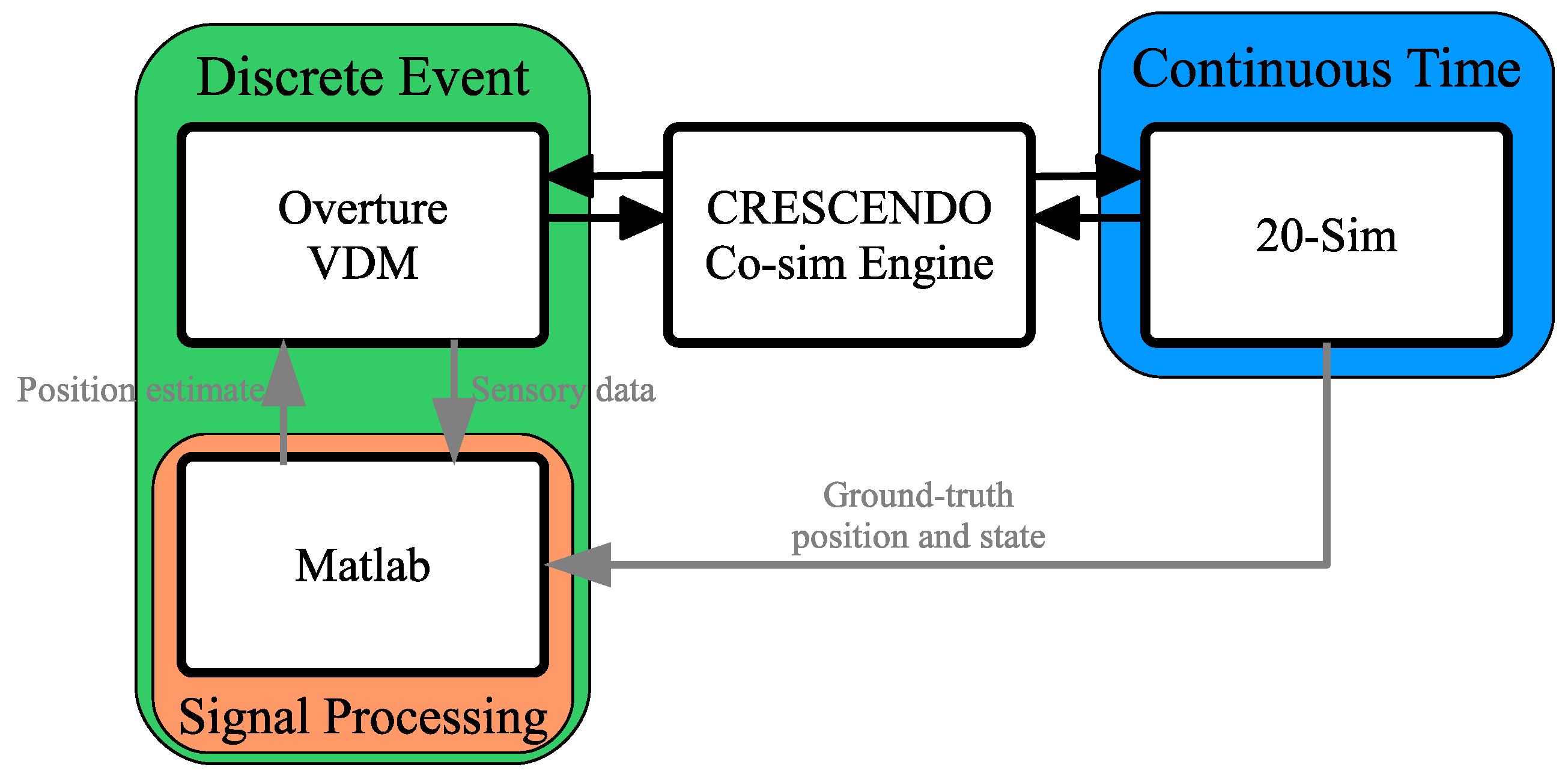
2. Co-Modeling Technologies
2.1. Crescendo Technology
2.2. MATLAB Extension

3. System Boundary Definition
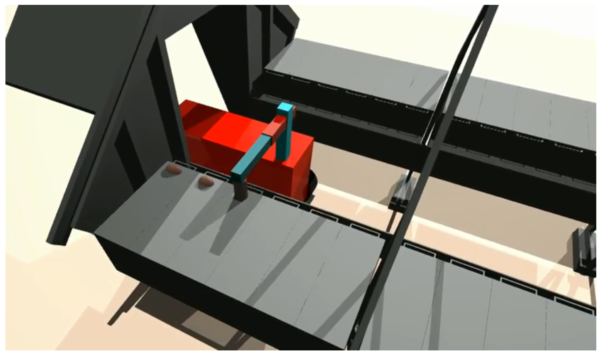
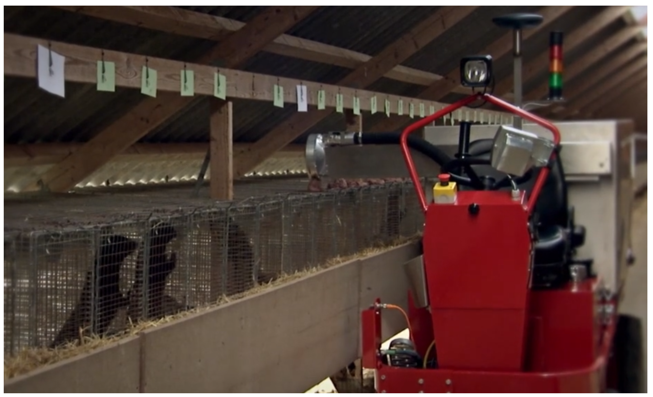
3.1. Problem Area Definition

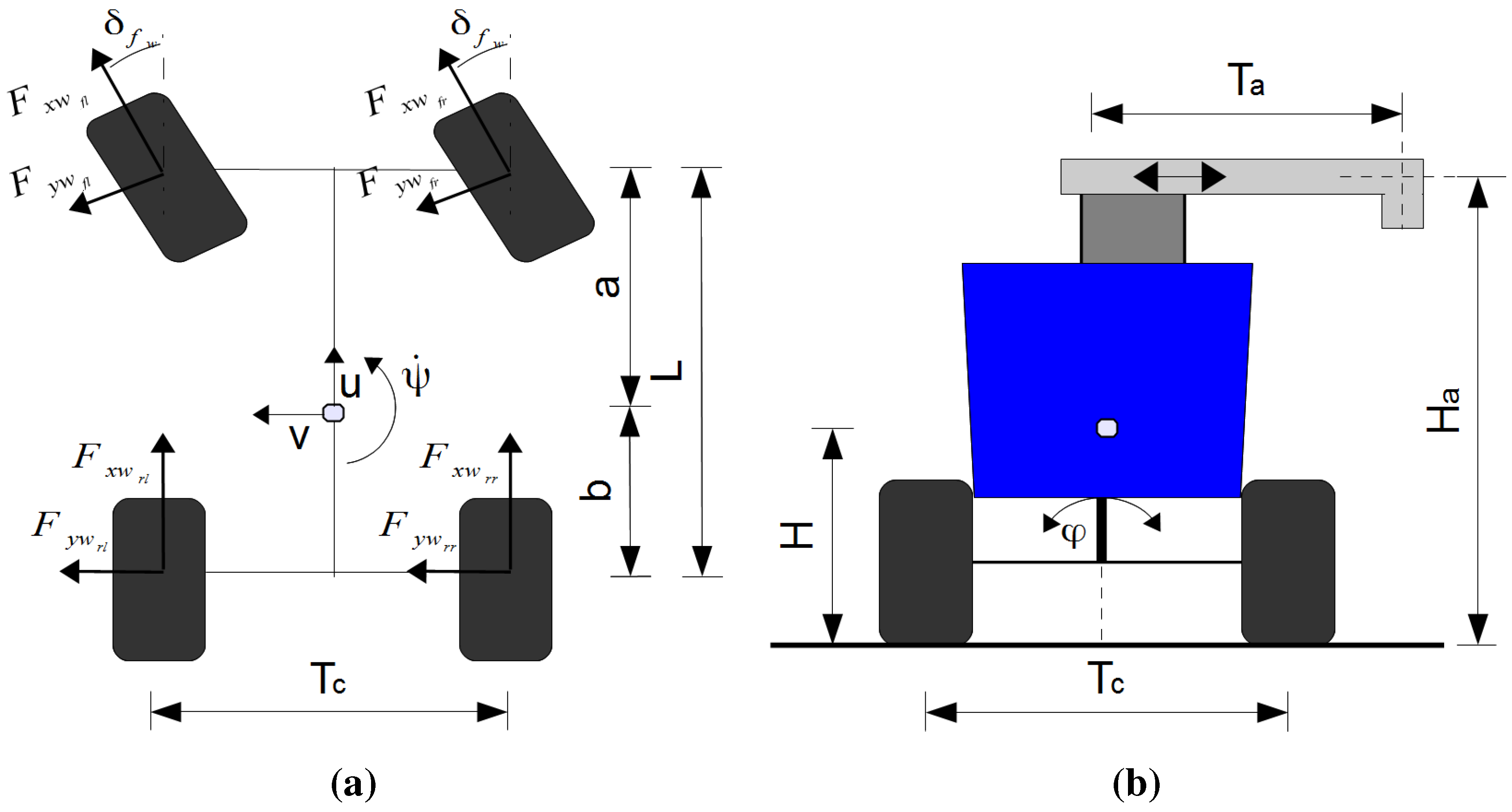
3.2. System Configuration and Performance Demands
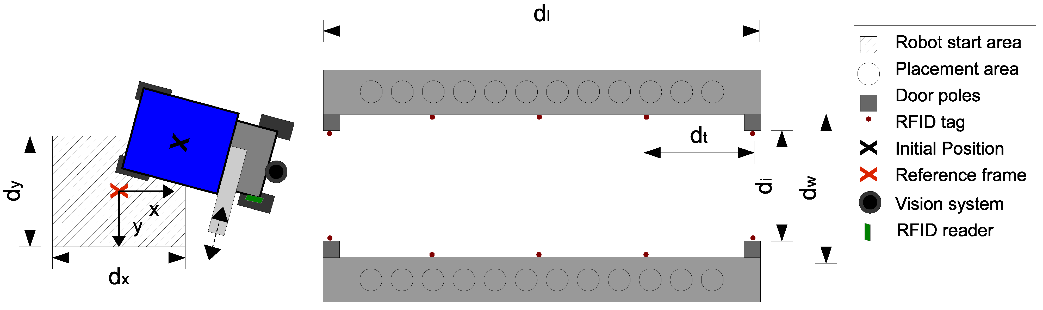
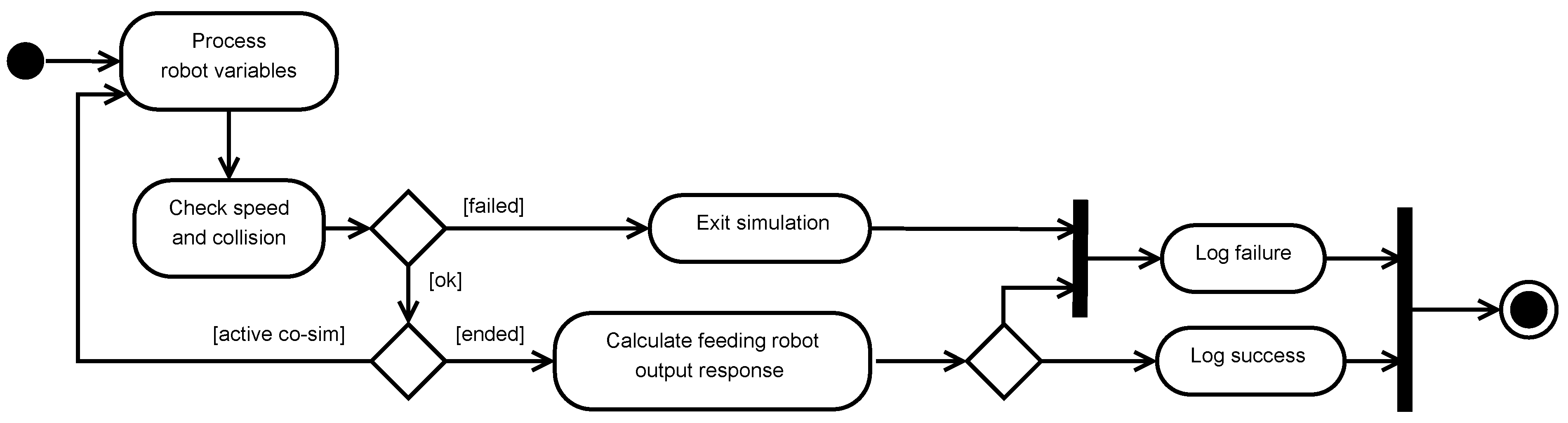
3.3. Modeling Cases
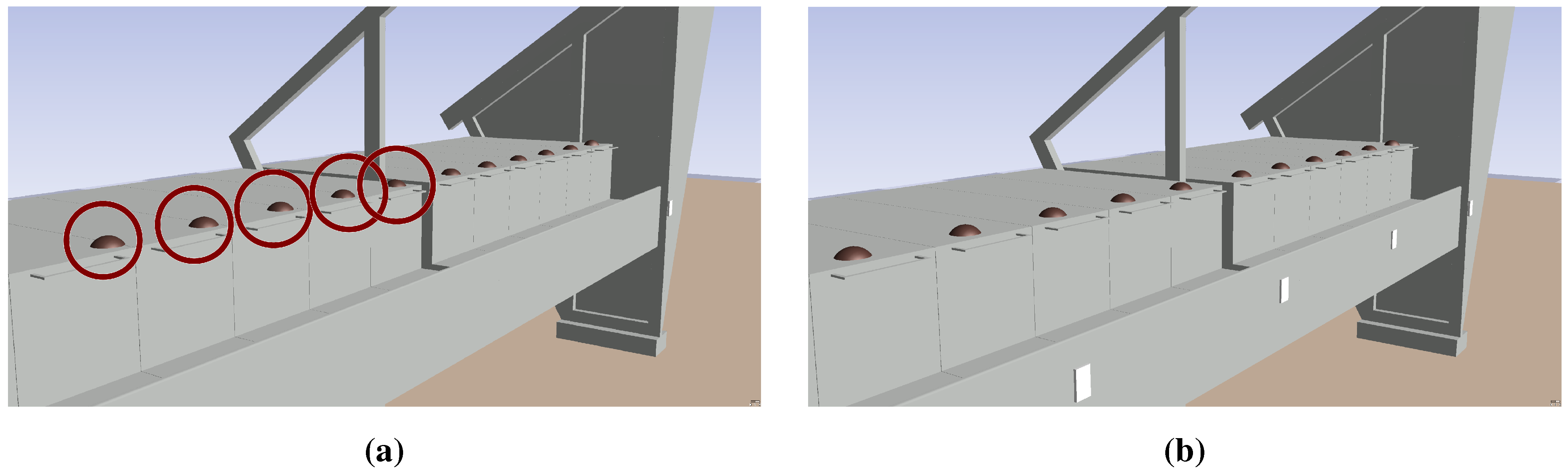
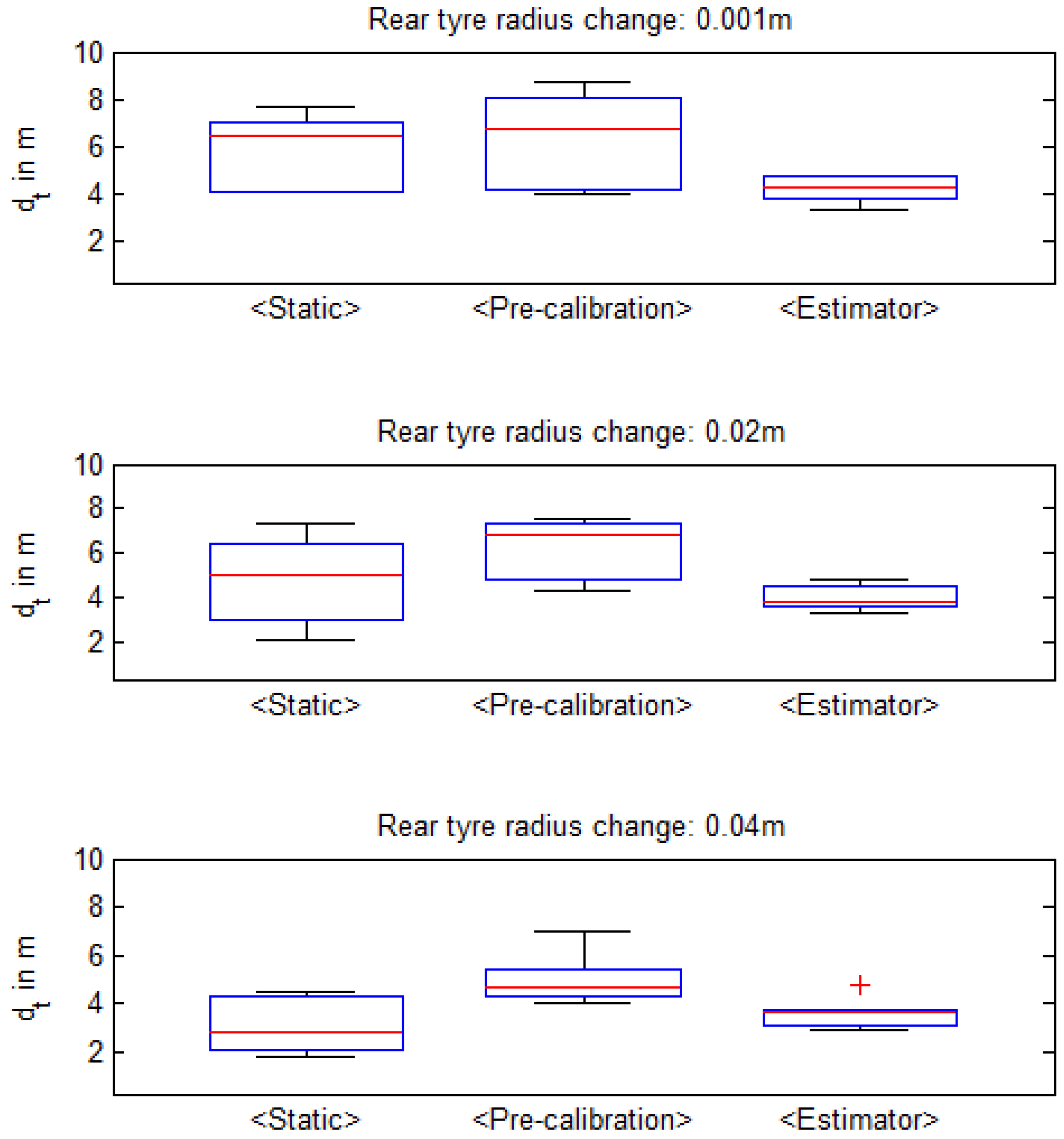
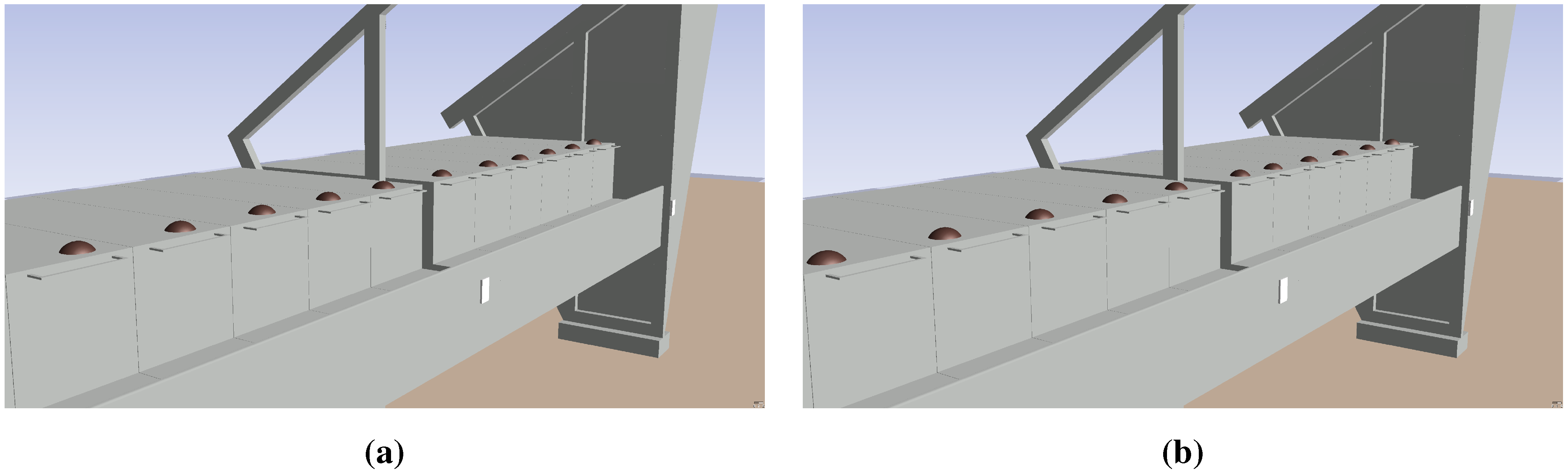
- <Static> The estimated effective tire radius was considered to be the mean of the values for the unloaded and fully-loaded robot. This is based on the assumption that the mean value will produce the least overall error in the estimate.
- <Pre-calibration> A pre-measured estimate of the current rear tire wheel radius in relation to the transported load is used in the DE part of the co-model. The estimates of the effective radius were obtained through the MATLAB bridge and directly passed from 20-sim with an accuracy of ±0.001 m.
- <Estimator> The input data obtained by the vision sensor were used to estimate the current effective radius before entering the feeding area. This estimate was based on the distance traveled between the updates, with an accuracy of.

| System Configurations | Min-Mean-Max Test Set | |||
|---|---|---|---|---|
| Rear Tire | Vehicle | Load Mass | Tire Surface | Initial Position |
| Radius Change | State Estimate | μ friction | ||
| 0.001 m | <Static> | 1% (6 kg) | 0.3 | |
| 0.02 m | <Pre-calibration> | 50% (300 kg) | 0.5 | |
| 0.04 m | <Estimator> | 100% (600 kg) | 0.7 | |
4. Co-Modeling
4.1. Crescendo Contract
| Name | Type | Parameter Symbol | |
|---|---|---|---|
| sdp | Initial_Position | array | |
| sdp | Surface_Tyre | real | μ |
| sdp | Load_Mass | real | |
| sdp | Tag_dist | real | |
| controlled | Speed_out | real | |
| controlled | Steering_Wheel_Angle | real | |
| controlled | Feeder_arm_pos | real | |
| controlled | Feeder_output | real | |
| monitored | Vision | array | |
| monitored | RFID | array | |
| monitored | IMU | real | |
| monitored | Encoders_Back | array | |
| monitored | Encoder_Front | real |
4.2. Automatic Co-Model Analysis

5. CT Modeling
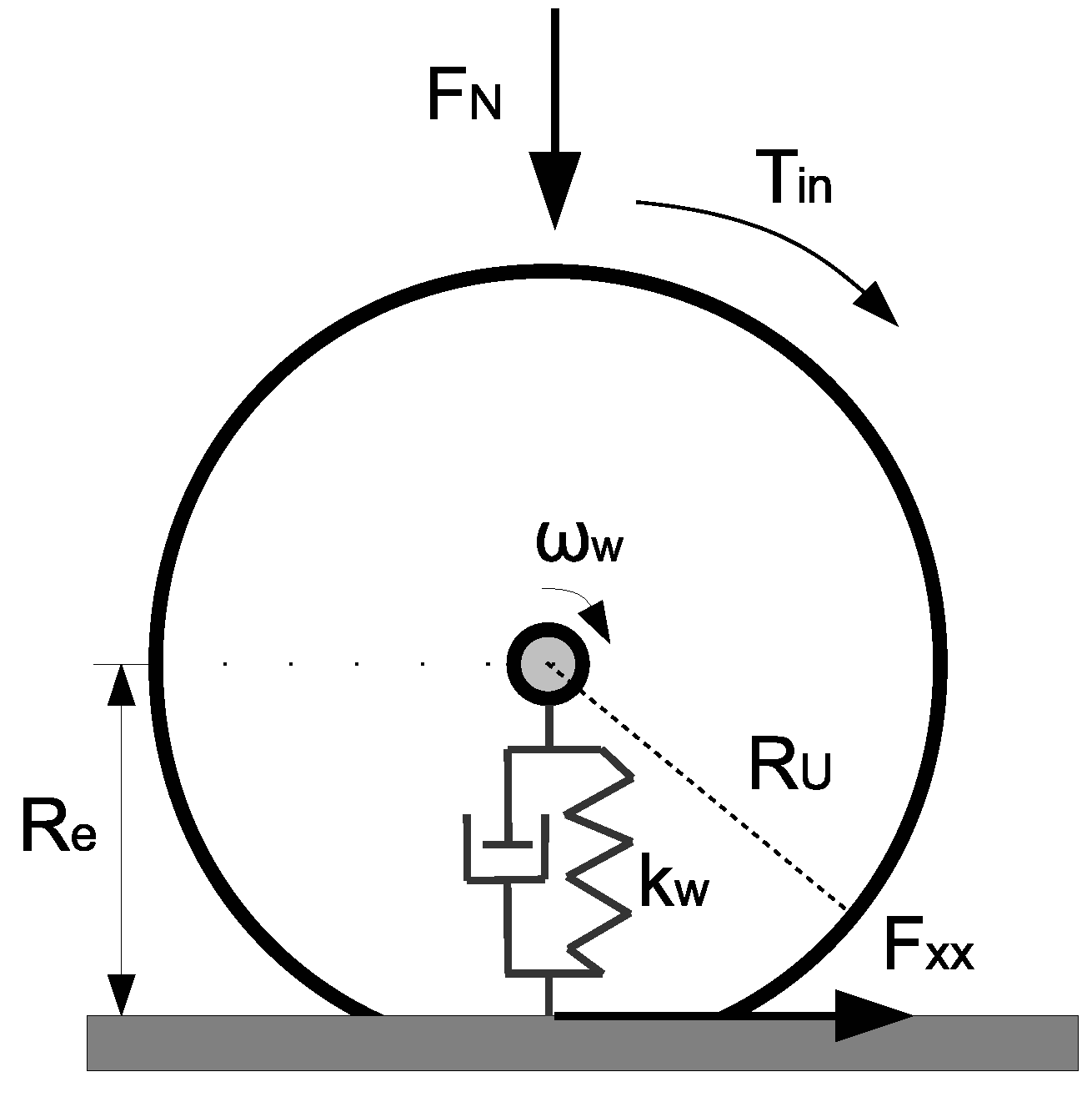
5.1. Tire Modeling for Encoder Data

5.2. Vehicle Body Dynamics
5.3. RFID Tag Reader
5.4. CT Setup
| Sub-System | Parameter Values |
|---|---|
| Environment | 20 m, 1.5 m, 1.34 m, |
| 1 m, 0.2 m | |
| Vehicle body | 2.1 m, 1.2 m, 0.9 m, 0.55 m, 0.65 m, 0.74 m, |
| 1.2 m, 800 kg, 600 kg, , | |
| , 0.3 m, , | |
| , | |
| Sensors | 4, 0.12 m, 0.16 m, 0.12 m |
| Encoder resolution = 13 bit, 5 m, 0.01 m, 0.005 m | |
| , |
6. DE Modeling
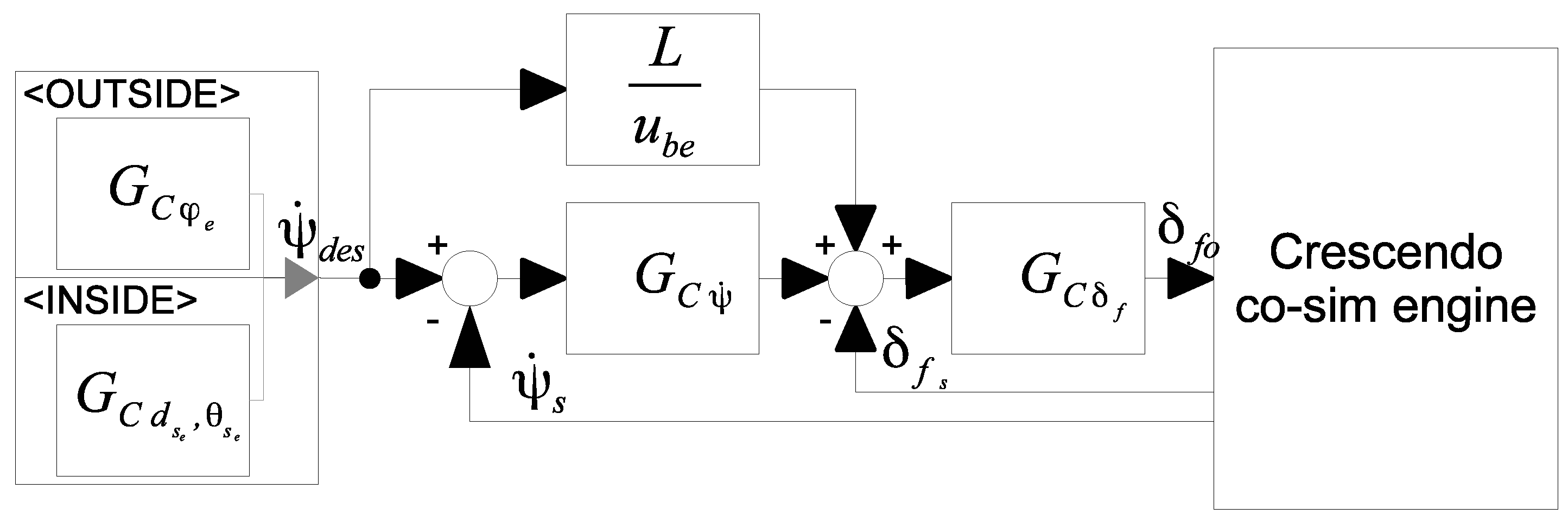
6.1. Control

6.2. Sensor Fusion
7. Results
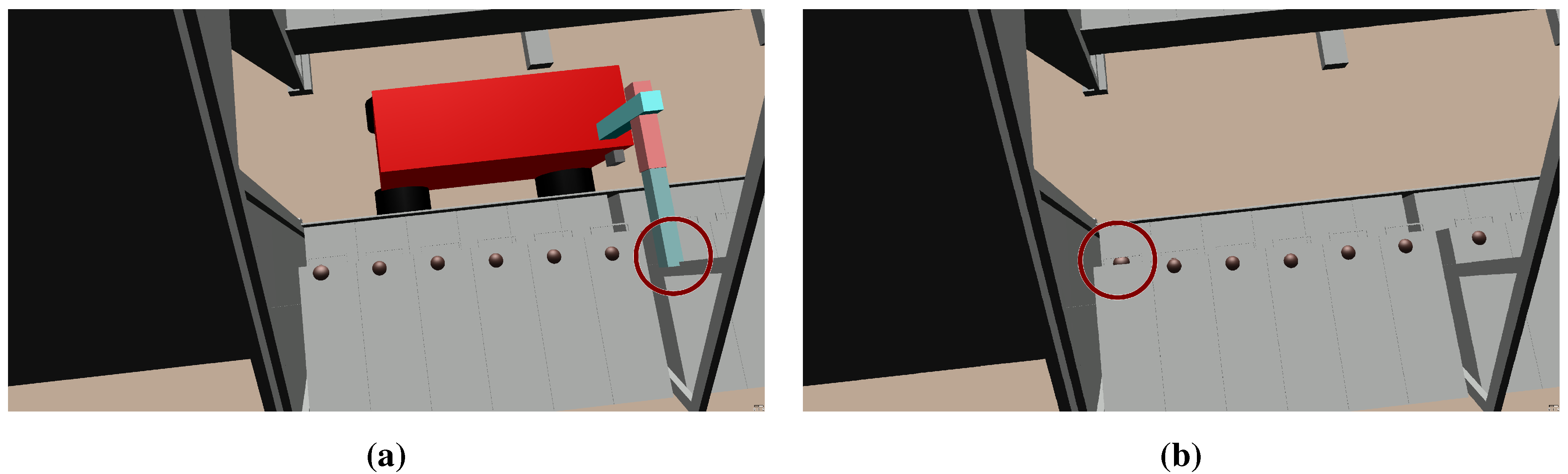
7.1. Selected Individual Results


8. Discussion
9. Concluding Remarks
Acknowledgments
Author Contributions
Conflicts of Interest
References
- Sørensen, C.; Jørgensen, R.; Maagaard, J.; Bertelsen, K.; Dalgaard, L.; Nørremark, M. Conceptual and user-centric design guidelines for a plant nursing robot. Biosyst. Eng. 2010, 105, 119–129. [Google Scholar] [CrossRef] [Green Version]
- Harris, A.; Conrad, J.M. Survey of popular robotics simulators, frameworks, and toolkits. In Proceedings of the 2011 IEEE Southeastcon, Nashville, TN, USA, 17–20 March 2011; IEEE: New York, NY, USA, 2011; pp. 243–249. [Google Scholar]
- Staranowicz, A.; Mariottini, G.L. A survey and comparison of commercial and open-source robotic simulator software. In Proceedings of the 4th International Conference on Pervasive Technologies Related to Assistive Environments—PETRA ’11, Crete, Greece, 25–27 May 2011; pp. 121–128.
- Longo, D.; Muscato, G. Design and Simulation of Two Robotic Systems for Automatic Artichoke Harvesting. Robotics 2013, 2, 217–230. [Google Scholar] [CrossRef]
- Murata, S.; Yoshida, E.; Tomita, K.; Kurokawa, H.; Kamimura, A.; Kokaji, S. Hardware design of modular robotic system. In Proceedings of the 2000 IEEE/RSJ International Conference on Intelligent Robots and Systems (IROS 2000) (Cat. No.00CH37113), Takamatsu, Japan, 31 October–5 November 2000; Volume 3, pp. 2210–2217.
- Baheti, R.; Gill, H. Cyber-Physical Systems. In The Impact of Control Technology; Samad, T., Annaswamy, A., Eds.; IEEE Control Society: New York, NY, USA, 2011; pp. 161–166. [Google Scholar]
- Pannaga, N.; Ganesh, N.; Gupta, R. Mechatronics—An Introduction to Mechatronics. Int. J. Eng. 2013, 2, 128–134. [Google Scholar]
- Piece, K.; Fitzgerald, J.; Gamble, C.; Ni, Y.; Broenink, J.F. Collaborative Modeling and Simulation—Guidelines for Engineering Using the DESTECS Tools and Methods. Technical Report, The DESTECS Project (INFSO-ICT-248134). Available online: http://destecs.org/images/stories/Project/Deliverables/D23MethodologicalGuidelines3.pdf (accessed on 24 September 2015).
- Fitzgerald, J.; Larsen, P.G.; Verhoef, M. Collaborative Design for Embedded Systems—Co-Modeling and Co-Simulation; Springer: Berlin, Germany, 2014. [Google Scholar]
- DESTECS (Design Support and Tooling for Embedded Control Software) homepage. Available online: http://destecs.org/ (accessed on 23 September 2015).
- Pierce, K.G.; Gamble, C.J.; Ni, Y.; Broenink, J.F. Collaborative Modeling and Co-Simulation with DESTECS: A Pilot Study. In Proceedings of the 3rd IEEE Track on Collaborative Modeling and Simulation, in WETICE 2012, Toulouse, France, 25–27 June 2012; IEEE-CS: New York, NY, USA, 2012. [Google Scholar]
- Abel, A.; Blochwitz, T.; Eichberger, A.; Hamann, P.; Rein, U. Functional Mock-up Interface in Mechatronic Gearshift Simulation for Commercial Vehicles. In Proceedings of the 9th International Modelica Conference, Munich, Germany, 3–5 September 2012.
- INTO-CPS (Integrated Tool Chain for Model-based Design of Cyber-Physical Systems) homepage. Available online: http://into-cps.au.dk/ (accessed on 23 September 2015).
- Fitzgerald, J.; Gamble, C.; Larsen, P.G.; Pierce, K.; Woodcock, J. Cyber-Physical Systems design: Formal Foundations, Methods and Integrated Tool Chains. In Proceedings of the FormaliSE: FME Workshop on Formal Methods in Software Engineering, ICSE 2015, Florence, Italy, 18 May 2015.
- Tan, C.; Kan, Z.; Zeng, M.; Li, J.B. RFID technology used in cow-feeding robots. J. Agric. Mech. Res. 2007, 2, 169–171. [Google Scholar]
- Jørgensen, R.N.; Sørensen, C.G.; Jensen, H.F.; Andersen, B.H.; Kristensen, E.F.; Jensen, K.; Maagaard, J.; Persson, A. FeederAnt2—An autonomous mobile unit feeding outdoor pigs. In Proceedings of the ASABE Annual International Meeting, Minneapolis, MN, USA, 17–20 June 2007.
- Nicolescu, G.; Boucheneb, H.; Gheorghe, L.; Bouchhima, F. Methodology for Efficient Design of Continuous/Discrete-Events Co-Simulation Tools. In Proceedings of the 2007 Western Multiconference on Computer Simulation WMC 2007, San Diego, CA, USA, 14–17 January 2007; Anderson, J., Huntsinger, R., Eds.; SCS: San Diego, CA, USA, 2007. [Google Scholar]
- Broenink, J.F.; Larsen, P.G.; Verhoef, M.; Kleijn, C.; Jovanovic, D.; Pierce, K. Design Support and Tooling for Dependable Embedded Control Software. In Proceedings of the Serene 2010 International Workshop on Software Engineering for Resilient Systems, London, UK, 13–16 April 2010; ACM: New York, NY, USA, 2010; pp. 77–82. [Google Scholar]
- The Crescendo tool homepage. Available online: http://crescendotool.org/. (accessed on 20 September 2015).
- Larsen, P.G.; Battle, N.; Ferreira, M.; Fitzgerald, J.; Lausdahl, K.; Verhoef, M. The Overture Initiative—Integrating Tools for VDM. SIGSOFT Softw. Eng. Notes 2010, 35, 1–6. [Google Scholar] [CrossRef]
- Bjørner, D.; Jones, C. The Vienna Development Method: The Meta-Language; Lecture Notes in Computer Science; Springer-Verlag: Berlin, Germany, 1978; Volume 61. [Google Scholar]
- Fitzgerald, J.S.; Larsen, P.G.; Verhoef, M. Vienna Development Method. In Wiley Encyclopedia of Computer Science and Engineering; Wah, B., Ed.; John Wiley & Sons, Inc.: New York, NY, USA, 2008. [Google Scholar]
- Kleijn, C. Modeling and Simulation of Fluid Power Systems with 20-sim. Int. J. Fluid Power 2006, 7, 1–6. [Google Scholar]
- Verhoef, M.; Larsen, P.G.; Hooman, J. Modeling and Validating Distributed Embedded Real-Time Systems with VDM++. In FM 2006: Formal Methods; Lecture Notes in Computer Science 4085; Misra, J., Nipkow, T., Sekerinski, E., Eds.; Springer-Verlag: Berlin, Germany; Heidelberg, Germany, 2006; pp. 147–162. [Google Scholar]
- Coleman, J.W.; Lausdahl, K.G.; Larsen, P.G. D3.4b—Co-simulation Semantics. Technical Report, The DESTECS Project (CNECT-ICT-248134). Available online: http://destecs.org/images/stories/Project/Deliverables/D34bCoSimulationSemantics.pdf (accessed on 24 September 2015).
- Kim, J.; Kim, Y.; Kim, S. An accurate localization for mobile robot using extended Kalman filter and sensor fusion. In Proceedings of the 2008 IEEE International Joint Conference on Neural Networks (IEEE World Congress on Computational Intelligence), Hong Kong, China, 1–8 June 2008; pp. 2928–2933.
- Raol, J.R. Multi-Sensor Data Fusion with MATLAB, 1st ed.; CRC Press: Boca Raton, FL, USA, 2009; p. 568. [Google Scholar]
- Guivant, J.; Nebot, E.; Whyte, H.D. Simultaneous Localization and Map Building Using Natural features in Outdoor Environments. Intell. Auton. Syst. 2000, 6, 581–586. [Google Scholar]
- Wulf, O.; Nuchter, A.; Hertzberg, J.; Wagner, B. Ground truth evaluation of large urban 6D SLAM. In Proceedings of 2007 IEEE/RSJ International Conference on Intelligent Robots and Systems, San Diego, CA, USA, 29 October–2 November 2007; pp. 650–657.
- Lin, H.H.; Tsai, C.C.; Chang, H.Y. Global Posture Estimation of a Tour-Guide Robot Using REID and Laser Scanning Measurements. In Proceedings of the 33rd Annual Conference of the IEEE Industrial Electronics Society, 2007, Taipei, Taiwan, 5–8 November 2007; pp. 483–488.
- Choi, B.S.; Lee, J.J. Mobile Robot Localization in Indoor Environment. In Proceedings of the IEEE/RSJ International Conference on Intelligent Robots and Systems, 2009, St. Louis, MO, USA, 10–15 October 2009; pp. 2039–2044.
- Zhou, J.; Shi, J. A comprehensive multi-factor analysis on RFID localization capability. Adv. Eng. Inf. 2011, 25, 32–40. [Google Scholar] [CrossRef]
- Marín, L.; Vallés, M.; Soriano, A.; Valera, A.; Albertos, P. Multi sensor fusion framework for indoor-outdoor localization of limited resource mobile robots. Sensors (Basel, Switzerland) 2013, 13, 14133–14160. [Google Scholar] [CrossRef] [PubMed]
- International Organization for Standardization (ISO). Robots for Industrial Environments—Safety Requirements—Part 1: Robot; Technical Report; The International Organization for Standardization and the International Electrotechnical Commission: London, UK, 2013. [Google Scholar]
- Chong, E.K.; Zak, S.H. An Introduction to Optimization, 3rd ed.; John Wiley & Sons: New York, NY, USA, 2008; p. 608. [Google Scholar]
- Thrun, S.; Burgard, W.; Fox, D. Probabilistic Robotics; MIT Press: Cambridge, MA, USA, 2005. [Google Scholar]
- Dugoff, H.; Fancher, P.S.; Segel, L. Tire Performance Characteristics Affecting Vehicle Response to Steering and Braking Control Inputs; Technical Report: Highway Safety Research Institute, University of Michigan, Ann Arbo, MI, USA, 1969. [Google Scholar]
- Bakker, E.; Pacejka, H.B.; Lidner, L. A New Tire Model with an Application in Vehicle Dynamics Studies. SAE Techni. Pap. 1989. [Google Scholar] [CrossRef]
- Pacejka, H.B.; Bakker, E. Shear Force Development by Pneumatic Tyres in Steady State Conditions: A Review of Modeling Aspects. Veh. Syst. Dyn. 1991, 20, 121–175. [Google Scholar] [CrossRef]
- Pacejka, H.B.; Bakker, E. The magic formula tire model. Veh. Syst. Dyn. 1992, 21, 1–18. [Google Scholar] [CrossRef]
- Bevly, D.M. GNSS for Vehicle Control, 1st ed.; Artech House: Norwood, MA, USA, 2009; p. 247. [Google Scholar]
- Marrocco, G.; di Giampaolo, E.; Aliberti, R. Estimation of UHF RFID Reading Regions in Real Environments. IEEE Antennas Propagat. Mag. 2009, 51, 44–57. [Google Scholar] [CrossRef]
- Nagasaka, Y.; Umeda, N.; Kanetai, Y.; Taniwaki, K.; Sasaki, Y. Autonomous guidance for rice transplanting using global positioning and gyroscopes. Comput. Electron. Agric. 2004, 43, 223–234. [Google Scholar] [CrossRef]
- Noguchi, N.; Ishii, K.; Terao, H. Development of an Agricultural Mobile Robot using a Geomagnetic Direction Sensor and Image Sensors. J. Agric. Eng. Res. 1997, 67, 1–15. [Google Scholar] [CrossRef]
- Hall, D.; Llinas, J. An introduction to multisensor data fusion. Proc. IEEE 1997, 85, 6–23. [Google Scholar] [CrossRef]
- Thrun, S. Is robotics going statistics? The field of probabilistic robotics. Commun. ACM 2001, 1, 1–8. [Google Scholar]
- Hansen, S.; Bayramoglu, E.; Andersen, J.C.; Ravn, O.; Andersen, N.; Poulsen, N.K. Orchard navigation using derivative free Kalman filtering. In Proceedings of the American Control Conference (ACC), San Francisco, CA, USA, 29 June–1 July 2011; IEEE: Newe York, NY, USA, 2011; pp. 4679–4684. [Google Scholar]
© 2015 by the authors; licensee MDPI, Basel, Switzerland. This article is an open access article distributed under the terms and conditions of the Creative Commons Attribution license (http://creativecommons.org/licenses/by/4.0/).
Share and Cite
Christiansen, M.P.; Larsen, P.G.; Jørgensen, R.N. Robotic Design Choice Overview Using Co-Simulation and Design Space Exploration. Robotics 2015, 4, 398-420. https://doi.org/10.3390/robotics4040398
Christiansen MP, Larsen PG, Jørgensen RN. Robotic Design Choice Overview Using Co-Simulation and Design Space Exploration. Robotics. 2015; 4(4):398-420. https://doi.org/10.3390/robotics4040398
Chicago/Turabian StyleChristiansen, Martin Peter, Peter Gorm Larsen, and Rasmus Nyholm Jørgensen. 2015. "Robotic Design Choice Overview Using Co-Simulation and Design Space Exploration" Robotics 4, no. 4: 398-420. https://doi.org/10.3390/robotics4040398