Adaptive Neuro-Fuzzy Technique for Autonomous Ground Vehicle Navigation

Abstract

This article proposes an adaptive neuro-fuzzy inference system (ANFIS) for solving navigation problems of an autonomous ground vehicle (AGV). The system consists of four ANFIS controllers; two of which are used for regulating both the left and right angular velocities of the AGV in order to reach the target position; and other two ANFIS controllers are used for optimal heading adjustment in order to avoid obstacles. The two velocity controllers receive three sensor inputs: front distance (FD); right distance (RD) and left distance (LD) for the low-level motion control. Two heading controllers deploy the angle difference (AD) between the heading of AGV and the angle to the target to choose the optimal direction. The simulation experiments have been carried out under two different scenarios to investigate the feasibility of the proposed ANFIS technique. The simulation results have been presented using MATLAB software package; showing that ANFIS is capable of performing the navigation and path planning task safely and efficiently in a workspace populated with static obstacles.

1. Introduction

Autonomous ground vehicles are an important key of industrial automation. Such vehicles could be utilized in different applications such as monitoring, transportation and many other potential applications. The path planning and navigation problems are one of area of current research. A considerable attention has been paid in recent years to deal with such problems. The autonomous vehicle must be able to gather and extract information from its surrounding using sensors. Thus, these sensors are fed to a controller to plan and execute its mission within its environment without human intervention [1].

The path planning methods are classified into either the global planning method or the local planning method [2]. In the global planning method, the autonomous vehicle requires the environment to be completely priori-known and the terrain should be static. In contrast, local path planning means the environment might be only partially known or completely unknown. In the local planning method, the autonomous ground vehicle utilises the received sensory information during its local navigation [3]. The autonomous ground vehicle must use sensors to perceive its surroundings and plan the motion.

In the current literature, many techniques have been used for solving the navigation and path planning problems. Some of the popular methods are the Visibility Graph algorithm [4], Voronoi Diagram [5], Bug Algorithm and the Potential Field method. For instance, in the potential field method, there is an attractive potential pulling the robot towards the goal point and a repulsive potential pushing the robot away from the obstacles over free space. However, the potential field method is prone to becoming stuck within local search minima.

In recent years, with the rapid development of modern computing techniques, artificial intelligence techniques have been applied widely in solving path planning and navigation problems. These techniques include genetic algorithm [6,7]. In [8], an obstacle avoidance control algorithm for mobile robots based on fuzzy controller was presented. The environment information surrounding the robot detected by the ultrasonic sensors is fuzzified, and then input into a fuzzy control system. The output of the fuzzy control system is used to drive the robot. The simulation results show that the algorithm can help the robot to avoid obstacles safely and is certainly feasible.

In [9], fuzzy logic controllers using different membership functions are developed and used to navigate mobile robots. First, a fuzzy controller was used with four types of input members, two types of output members and three parameters each. Next, two types of fuzzy controllers were developed having same input members and output members with five parameters each. Each robot had an array of ultrasonic sensors for measuring the distances of obstacles around it and an infrared sensor for detecting the bearing of the target. In [10], a fuzzy logic system was designed for a path planning in an unknown environment for a mobile robot. The ultrasonic sensors were employed for detecting the distance and positions of obstacles. An angular velocity control for left and right wheels was implemented by a fuzzy logic system. This included another new rule table that was induced from the consideration of the distance to obstacles and the angle between the robot and the goal.

In [11], an obstacle avoidance approach for an e-puck robot by using fuzzy logic controller was introduced. The inputs from eight IR sensors and the output of the motor speed were used to construct the fuzzy logic rules. A Webots Pro Simulation software was used to model and program the e-puck robot and fuzzy algorithm and to test an environment. Chi and Less [12], showed an artificial neural networks was applied to learn the environment from sensory data to move along a collision free trajectory. In [13], the navigation of non-holonomic robot was discussed using neuro-fuzzy. The ANFIS parameters were discovered offline by using suitable datasets and the obtained parameters were fed into the robot.

Joshi and Zaveri [14], showed a neuro-fuzzy based system for the behaviour based control of a mobile robot for reactive navigation. Systems transform sensors’ input to yield wheel velocities using behaviour based fuzzy reasoning. Singh et al. [15], analysed an adaptive neuro-fuzzy technique for the navigation of a mobile robot in unknown environment. The results improved the validity of the proposed technique to determine the optimal time and create a collision free path of the mobile robot. In [16], a hybrid neuro-genetic fuzzy technique was proposed for choosing the collision free path form a set of paths. Fuzzy logic was used for obstacle avoidance when a neural network is unable to choose a path due to blockage from obstacles in a number of sets of directions.

From the literature survey, it can be clearly seen that several issues have not been addressed yet. Firstly, the consideration of the physical dimensions of the autonomous ground vehicle (length and width); authors normally assume the vehicle is a point in a workplace. Secondly, the online sensing information from the three directions (front, right, left) during the navigation. Thirdly, the problem of the complexity of the navigation environment. Therefore, in this paper, all aforementioned issues have been involved to create a new problem formulation for solving the navigation problem in a complex static environment contains multiple obstacles with different shapes and sizes.

The contribution of the proposed approach can be understood as the implementing a new ANFIS model which has the ability to avoid becoming stuck into local minimum and generates a smooth trajectory between the starting and the target points in unknown environment based local planning method. In other words, the ANFIS model successfully and efficiently guide the vehicle through the workspace. Moreover, the performance of the ANFIS controller is verified by changing the poses of obstacles.

The work in this paper is divided in two stages: firstly, the target reaching controller, and secondly, the obstacle avoidance controller. The target reaching controller was implemented using two ANFIS controllers. Each controller received the same input, which was the angle difference between the autonomous ground vehicle’s direction and the target’s angle. The output of first ANFIS controller was used to control the right angular velocity, and the second ANFIS controller was used to control the left angular velocity. The obstacle avoidance controller was also implemented also using two ANFIS controllers. Each controller received three inputs that represent the front, right and left distances. These distances represent sensory information between the autonomous vehicle and obstacles. The paper is organized as follows: Section 2 describes a kinematic model of an autonomous ground vehicle. The architecture of neuro-fuzzy inference system is presented in Section 3. The design of adopted four ANFIS controllers and autonomous ground vehicle platform are described in Section 4. To validate the proposed approach, simulation results are conducted and discussed in Section 5. Finally, the conclusions are presented in Section 6.

2. The Kinematic Model of an Autonomous Ground Vehicle

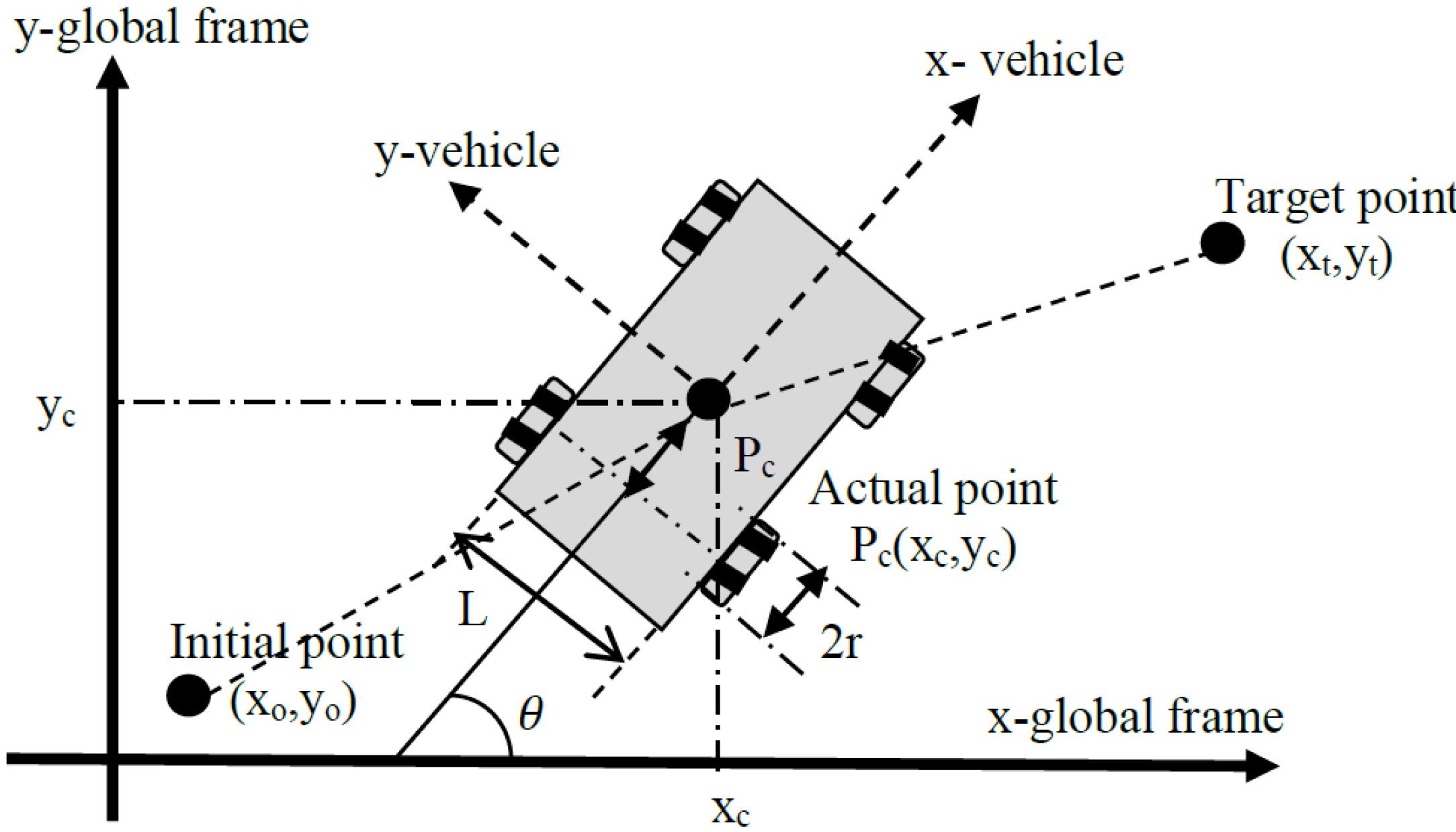
The schematic diagram of a two-dimensional plane for an autonomous ground vehicle is shown in Figure 1. The initial Cartesian coordinates for this vehicle are x_o in x-axis and y_o in y-axis. Similarly, target point coordinates are denoted as x_t and y_t respectively. The vehicle’s current position is coordinate P_c. The vehicle has four fixed standard wheels and is differentially driven by skid steer motion. The wheels have the same radius, r. The driving wheels are separated by a distance L. In general, the posture of the vehicle in the two dimensional plane at any instant is defined by the systems Cartesian coordinates and heading angle, $\theta$, with respect to a global frame reference, Pc = (x_c, y_c, $\theta$). In this paper, the wheels’ radius equals r = 0.1 m, and the distance between the driving wheels equals L = 0.3 m. It is assumed that the autonomous ground vehicle is subject to the kinematic constraints such as the contact between the wheels and the ground is pure rolling, and non-slipping [17]. Such constraints cause some challenge in the motion planning.

Figure 1. The schematic diagram of the autonomous ground vehicle.

Figure 1. The schematic diagram of the autonomous ground vehicle.

A set of relationships for the autonomous ground vehicle can be defined as:

• No slip constraint

  $$\dot{x_c}\left(t\right)\cos \theta \left(t\right)- \dot{y_c}\left(t\right)\sin \theta \left(t\right) =a \dot{\theta }\left(t\right)$$

  (1)
• Pure rolling constraint

  $$\dot{x_c}\left(t\right)\cos \theta \left(t\right)+ \dot{y_c}\left(t\right)\sin \theta \left(t\right)+ L \dot{\theta }\left(t\right)=r \dot{{\varnothing }_r}\left(t\right)$$

  (2)

  $$\dot{x_c}\left(t\right)\cos \theta \left(t\right)+ \dot{y_c}\left(t\right)\sin \theta \left(t\right)- L \dot{\theta }\left(t\right) =r \dot{{\varnothing }_l}\left(t\right)$$

  (3)

  $$\left[\begin{array}{c}{v}_x\left(t\right)\\ v_y\left(t\right)\\ \dot{\theta }\left(t\right)\end{array}\right]=\left[\begin{array}{cc}\frac{r}{2} & \frac{r}{2}\\ 0 & 0\\ -\frac{r}{L} & \frac{r}{L}\end{array}\right]\left[\begin{array}{c}{w}_l\left(t\right)\\ w_r\left(t\right)\end{array}\right]$$

  (4)

  $$v\left(t\right)=r. \frac{w_r\left(t\right)+w_l\left(t\right)}{2}$$

  (5)

  $$\dot{\theta }\left(t\right)=r.\left[\frac{w_r\left(t\right)-w_l\left(t\right)}{L} \right]$$

  (6)

  $$\dot{x}\left(t\right)=v\left(t\right)\cos \theta \left(t\right)$$

  (7)

  $$\dot{y}\left(t\right)=v\left(t\right)\sin \theta \left(t\right)$$

  (8)

  $$w\left(t\right)=\dot{\theta }\left(t\right) \left(9\right)$$

  (9)

  $${\mathrm{w}}_{\mathrm{r}}\left(\mathrm{t}\right)= \dot{{\varnothing }_r}\left(t\right)$$

  (10)

  $${\mathrm{w}}_{\mathrm{l}}\left(\mathrm{t}\right)=\dot{{\varnothing }_l}\left(t\right)$$

  (11)

  $$\text{or }\left[\begin{array}{c} \dot{x}\left(t\right)\\ \dot{y}\left(t\right)\\ \dot{\theta }\left(t\right)\end{array}\right]=\left[\begin{array}{cc}cos\theta & 0\\ Sin\theta & 0\\ 0 & 1\end{array}\right]\left[\begin{array}{c}V\\ w\end{array}\right]$$

  (12)

  where,

  • ${\mathrm{v}}_{\mathrm{x}}\left(\mathrm{t}\right)$ = longitudinal velocity of the moving vehicle [m/s]
  • ${\mathrm{v}}_{\mathrm{y}}\left(\mathrm{t}\right)$ = lateral velocity of the moving vehicle [m/s]
  • $\text{θ}$ = moving vehicle orientation [degree]
  • ${\mathrm{w}}_{\mathrm{r}}\left(\mathrm{t}\right)$ = angular velocity of right wheel [rad/s]
  • ${\mathrm{w}}_{\mathrm{l}}\left(\mathrm{t}\right)$ = angular velocity of left wheel [rad/s]
  • $\mathrm{w}\left(\mathrm{t}\right)$ = angular velocity of vehicle [rad/s]
  • r = wheel radius [m]
  • a = the distance between the centre of mass and driving wheels axis in x-direction [m]
  • L = the distance between each driving wheel and the vehicle axis of symmetry in y-direction [m].

3. The Architecture of Adaptive Neuro-Fuzzy Inference System (ANFIS)

The architecture of the ANFIS technique, consists of the fuzzy inference system and neural network with given input and output data pairs. This technique is a self-tuning and adaptive hybrid controller that uses learning algorithms. In other words, this technique gives the fuzzy logic capability to adapt the membership function parameters that best allow the associated fuzzy inference system to track the given input and output data parameters of ANFIS model. In order to process a fuzzy rule by neural networks, it is necessary to modify the standard neural network structure accordingly. 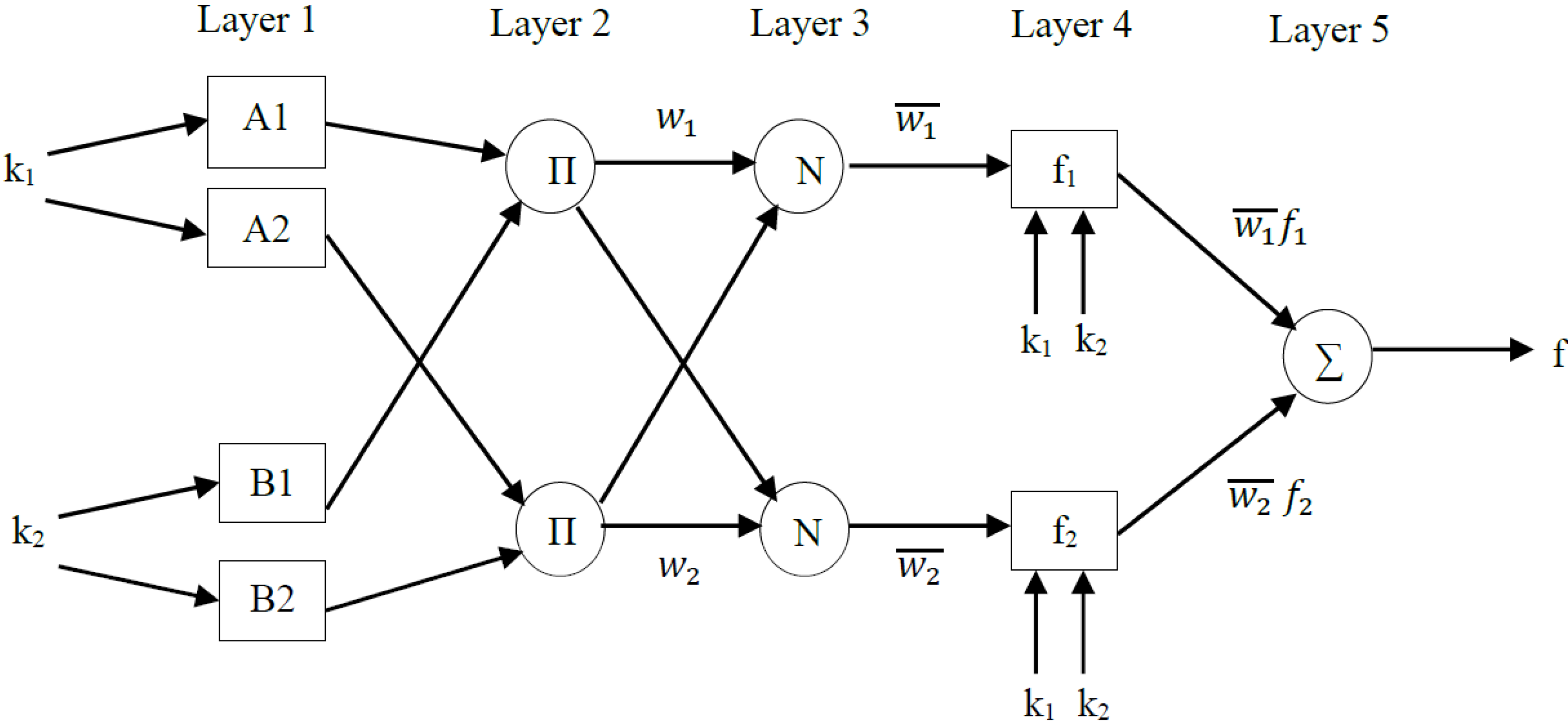Figure 2 depicts the architecture model of ANFIS. This model is called a first-order Takagi-Sugeno-fuzzy model [18]. For simplicity, it is assumed that the ANFIS model has two inputs k₁ and k₂, and one output f.

Figure 2. The architecture of an adaptive neuro-fuzzy inference system (ANFIS).

Figure 2. The architecture of an adaptive neuro-fuzzy inference system (ANFIS).

This system is broken down into five layers:

Layer 1: Every node i in this layer is an adaptive node with a node function

$$O_{1,i}={\mu }_{A\_i}\left(x\right),fori=1,2$$

(13)

$$O_{1,i}={\mu }_{B_{i-2}}\left(y\right),fori=3,4$$

(14)

where $k_1$ (or $k_2$) is the input to node i and A_i (or B_i-2) is a linguistic label (such as "small" or "large") associated with this node. In other words, O_1,i is the membership grade of a fuzzy set A ( = A₁ , A₂ , B₁ or B₂ ) and it specifies the degree to which the given input $k_1$ (or $k_2$) satisfies the quantifier A. Here the membership function for A is assumed be triangular shaped membership function:

$${\mu }_A\left(x\right)=max\left[min\left\{\frac{x-a_i}{b_i-a_i},\frac{c_i-x}{c_i-b_i}\right\},0\right]$$

(15)

where {a_i, b_i, c_i} is the parameter set. As the values of these parameters change, the bell-shaped function varies accordingly, thus exhibiting various forms of membership function for fuzzy set A. Parameters in this layer are referred to as premise parameters.

Layer 2: Every node in this layer is a fixed node labelled Π, whose output is the product of all the incoming signals:

$$O_{2,i}=w_i={\mu }_{A\_i}\left(x\right){\mu }_{B_i}\left(y\right),i=1,2$$

(16)

Each node output represents the firing strength of a rule. In general, any other T-norm operators that perform a fuzzy AND can be used as the node function in this layer.

Layer 3: Every node in this layer is a fixed node labelled N. The i^th node calculates the ratio of the i^th rule’s firing strength to the sum of all of the rules firing strengths:

$$O_{3,i}=\overline{w_i}=\frac{w_i}{w_1+w_2}i=1,2$$

(17)

The output of this layer is called the normalised firing strengths.

Layer 4: Every node i in this layer is an adaptive node with a node function:

$$O_{4,i}=\overline{w_i}{f}_i=\overline{w_i}\left(p_{i}x+q_{i}y+r_i\right), i=1,2$$

(18)

where $\overline{w_i}$ is the normalised firing strength from layer 3 and {p_i, q_i, r_i} is the parameter set of this node. Parameters in this layer are referred to as consequent parameters.

Layer 5: The single node in this layer is a fixed node labelled ∑, which computes the overall output, f, as the summation of all incoming signals:

$$f=O_{5,1}={\displaystyle \sum }_i\overline{w_i}{f}_i=\frac{{{\displaystyle \sum }}_i{w}_i{f}_i}{{{\displaystyle \sum }}_i{w}_i} i=1,2$$

(19)

The first and fourth layers are adaptive layers in the ANFIS architecture. The modifiable parameters are called premise parameters in the first layer and consequent parameters in the fourth layer. The task of learning is to tune all modifiable parameters to make the ANFIS match the training data. In this paper, the trainable parameters of ANFIS, i.e., premise parameters and consequent parameters {a_i, b_i, c_i} and {p_i, q_i, r_i} are adjusted to make the ANFIS output match the training data. The adopted hybrid learning technique combines the least square method and gradient descent method in ANFIS Toolbox. The hybrid learning algorithm is composed of a forward pass and a backward pass. The least squares method (forward pass) is used to optimize the consequent parameters with the premise parameters fixed. Once the optimal consequent parameters are found, the backward pass starts immediately. The gradient descent method (backward pass) is used to adjust optimally the premise parameters corresponding to the fuzzy sets in the input domain. The output of the ANFIS is calculated by employing the consequent parameters found in the forward pass. The output error is used to adapt the premise parameters by means of a standard back propagation algorithm. It has been proven that this hybrid algorithm is highly efficient in training the ANFIS.

4. Design of the Autonomous Ground Vehicle’s ANFIS Controller

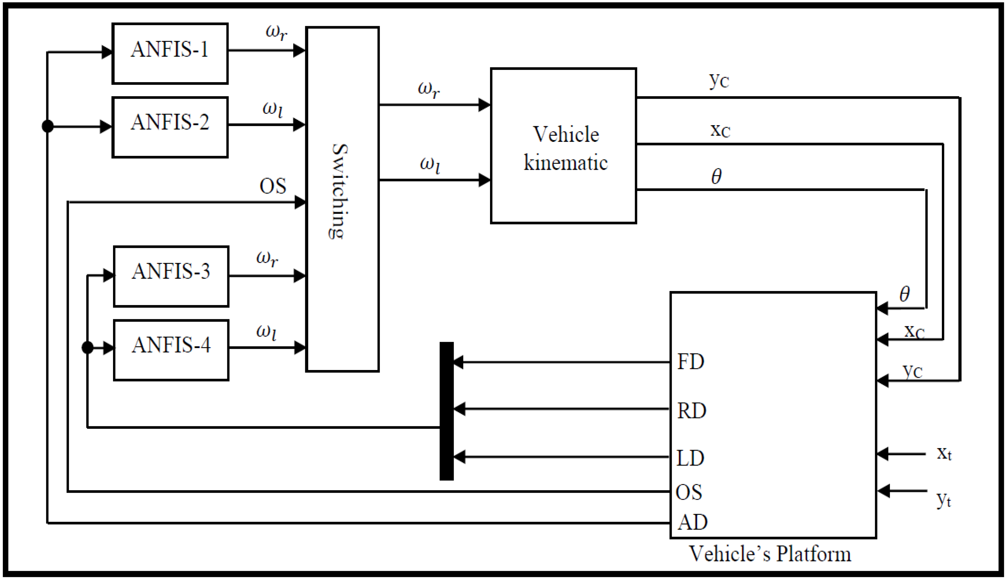
In this section, the proposed ANFIS controllers are discussed in detail. There are four ANFIS controllers which have been designed to accomplish the navigation task; firstly, two ANFIS controllers for achieving the target reaching task, secondly, the other two ANFIS controllers for performing the obstacle avoidance mission.

All four controllers will be combined through a switch block for choosing which controller will be activated. For instance, if there are no obstacles in the vehicle’s path, the target reaching controller will be activated. Otherwise, if the vehicle senses an obstacle, the obstacle avoidance controller will be activated. The switching between these two controllers will be decided according to an obstacle sensing signal, OS, from an environment model. This signal is generated in accordance to measured distances (front, right, and left) from sensory information. If the vehicle does not sense an obstacle in its path, this OS parameter will indicate ‘0’ if there is no an obstacle and ‘1’ if the vehicle senses an obstacle near to its platform. Thus, the output of the switching block will be the angular velocities of the left and right wheel of the autonomous ground vehicle. These velocities are fed into the vehicle model in order to obtain the instantaneous vehicle’s posture through the movement of the vehicle. Figure 3 depicts the structure of the proposed ANFIS controllers based navigation systems with the autonomous ground vehicle and the implemented workspace.

Figure 3. The structure of the proposed ANFIS and the autonomous ground vehicle.

Figure 3. The structure of the proposed ANFIS and the autonomous ground vehicle.

4.1. Autonomous Ground Vehicle Platform

The autonomous ground vehicle utilized in this paper is equipped with four wheels. The right and left back wheels drive independently. Two encoders are fixed on the back axis for the left and right wheel in order to measure the instantaneous position of the vehicle. The platform is created by using the Matlab-Simulink software package. This software has a vast diversity of tools that used for technical computing and interface graphical implementations. The implementation of this platform is illustrated in Figure 4. As show in the figure the vehicle has three degrees of freedom that are represented by the vehicle’s posture (x_c, y_c, $\theta$) in the global coordinate system. The s-function is a Matlab Simulink block was used to create the platform. As illustrated in the Figure 4, the Simulink block receives six inputs and produces five outputs. The platform parameters are explained below:

Remark 1. The front, right and left distances (FD, RD, and LD) represent the shortest distance between the vehicle and obstacles in the front, right and left directions respectively. The sensory information is modelled by assuming these three sensors are placed on a vehicle’s platform, and each senor carries the information for three directions of the platform. These sensor outputs change depending on the distance between the instantaneous positions of the vehicle.

Remark 2. The angle difference (AD) represents the difference between the vehicle’s heading and the target point.

Remark 3. Obstacle sensing (OS) signal is generated in accordance to the measured distances (front, right, left) from the sensory information. If the vehicle does not sense an obstacle in its path, this OS parameter will indicate ‘0’ if there is no an obstacle, and ‘1’ if the vehicle senses an obstacle near to its platform.

Remark 4. The clock timer is used for measuring the simulation running time that the vehicle elapsed to reach the destination in the platform.

Figure 4. The Schematic diagram for the autonomous ground vehicle platform.

Figure 4. The Schematic diagram for the autonomous ground vehicle platform.

4.2. Target Reaching ANFIS Controller

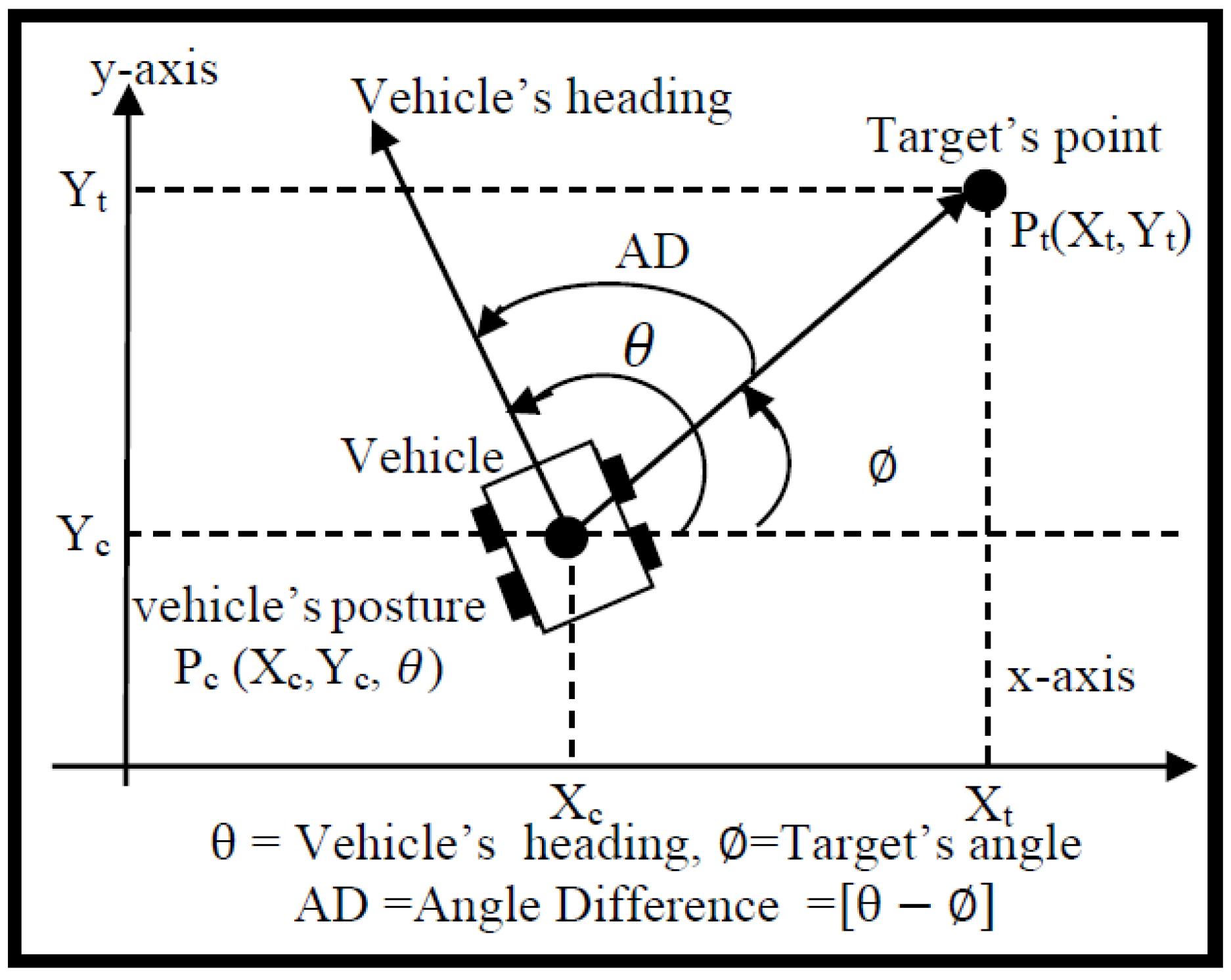
To achieve the target reaching mission, two ANFIS controllers are implemented to drive the right and left angular velocities. The input of this controller is the angle difference, AD. This angle represents the difference between the vehicle’s heading and the target’s point. The calculation of this angle is depicted in Figure 5. The output of the first controller is the right angular velocity and for the second controller is the left angular velocity. In this study, a total of 40 sets of data range were selected for implemented the target-reaching controller for the purpose of training the ANFIS. 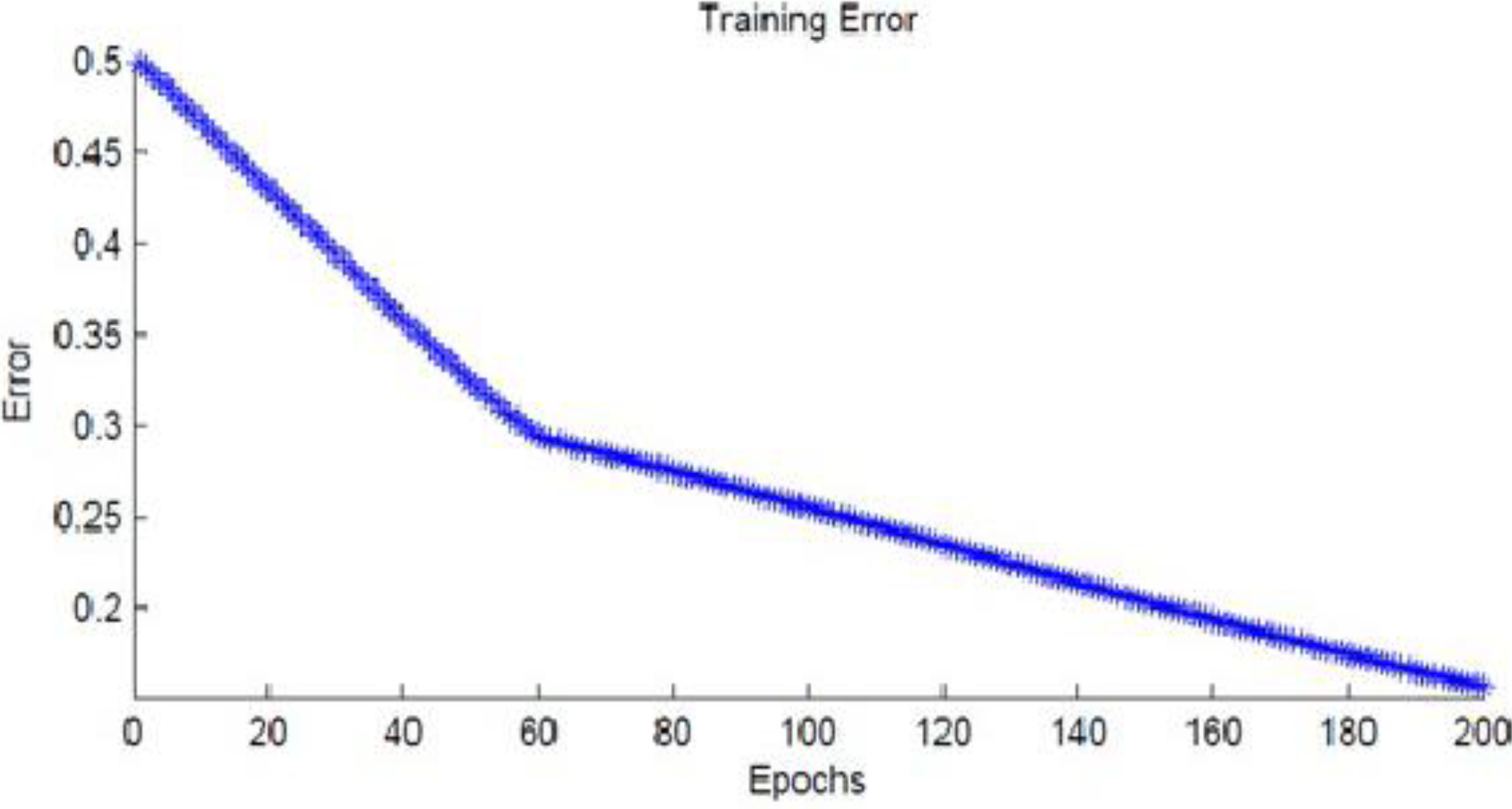The training data for input and outputs ranges are given in Table 1. This training adjusts the membership parameters to implement the required model. The ANFIS learning information for predicting the angular velocity for the left and the right wheels are as follows: number of nodes, 52; number of linear parameters, 12; number of nonlinear parameters, 36; total number of parameters, 48; number of fuzzy rules, 12. Training results shows that the average error for predicting angular velocity is 0.15631 rad/s with an epoch number of 200. The epoch value is chosen after a number of iteration for obtaining the minimum value of error between the input and local set points. The relation between the average error and epoch number is given in Figure 6. 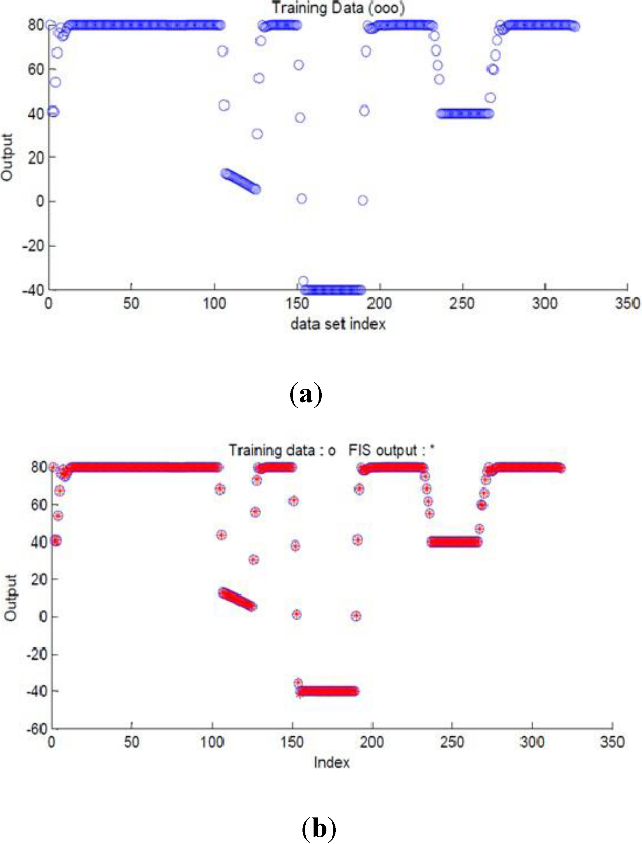Figure 7a,b shows the output training data for obstacle avoidance ANFIS initially before the training and after the training process is completed.

Figure 5. Coordinates for moving to a target point.

Figure 5. Coordinates for moving to a target point.

Table 1. Training data of target reaching ANFIS controller.

Item Number	Angle Difference	Right Angular Velocity	Left Angular Velocity
1	0	80	80
2	−44.007	40.882	−37.352
3	−29.214	54.031	2.093
4	−14.226	67.353	42.061
5	−4.319	76.160	68.480
6	0.505	78.652	79.550
7	1.975	74.731	78.243
8	1.809	75.173	78.391
9	0.530	78.584	79.528
10	−0.009	79.991	79.974
11	4.4693	68.081	76.027
12	13.668	43.550	67.850
13	25.192	12.819	57.606
14	26.956	8.116	56.038
15	27.114	7.694	55.898
16	18.5223	30.607	63.535
17	9.047	55.873	71.957
18	2.774	72.602	77.534
19	−0.295	79.737	79.211
20	6.759	61.975	73.991
21	15.705	38.117	66.039
22	29.555	1.186	53.728
23	43.460	−35.895	41.368
25	55.161	−40	40
26	62.435	−40	40
27	14.562	41.167	67.055
28	4.477	68.058	76.019
29	−5.788	74.854	64.563
30	−13.107	68.348	45.046
31	−20.435	61.835	25.505
32	−27.755	55.328	5.985
33	−85.460	40	−40
34	−37.315	46.830	−19.507
35	−22.376	60.110	20.330
36	−22.843	59.694	19.082
37	−15.563	66.165	38.496
38	−7.999	72.888	58.66
39	−2.812	77.500	72.500
40	0.2973	79.207	79.735

Table 1. Training data of target reaching ANFIS controller.

Item Number	Angle Difference	Right Angular Velocity	Left Angular Velocity
1	0	80	80
2	−44.007	40.882	−37.352
3	−29.214	54.031	2.093
4	−14.226	67.353	42.061
5	−4.319	76.160	68.480
6	0.505	78.652	79.550
7	1.975	74.731	78.243
8	1.809	75.173	78.391
9	0.530	78.584	79.528
10	−0.009	79.991	79.974
11	4.4693	68.081	76.027
12	13.668	43.550	67.850
13	25.192	12.819	57.606
14	26.956	8.116	56.038
15	27.114	7.694	55.898
16	18.5223	30.607	63.535
17	9.047	55.873	71.957
18	2.774	72.602	77.534
19	−0.295	79.737	79.211
20	6.759	61.975	73.991
21	15.705	38.117	66.039
22	29.555	1.186	53.728
23	43.460	−35.895	41.368
25	55.161	−40	40
26	62.435	−40	40
27	14.562	41.167	67.055
28	4.477	68.058	76.019
29	−5.788	74.854	64.563
30	−13.107	68.348	45.046
31	−20.435	61.835	25.505
32	−27.755	55.328	5.985
33	−85.460	40	−40
34	−37.315	46.830	−19.507
35	−22.376	60.110	20.330
36	−22.843	59.694	19.082
37	−15.563	66.165	38.496
38	−7.999	72.888	58.66
39	−2.812	77.500	72.500
40	0.2973	79.207	79.735

Figure 6. Relationship between training error and epoch’s number for the target-reaching ANFIS controller.

Figure 6. Relationship between training error and epoch’s number for the target-reaching ANFIS controller.

Figure 7. The output data for target reaching ANFIS controller. (a) The initial data before the training (b). The matched data after the ANFIS is trained.

Figure 7. The output data for target reaching ANFIS controller. (a) The initial data before the training (b). The matched data after the ANFIS is trained.

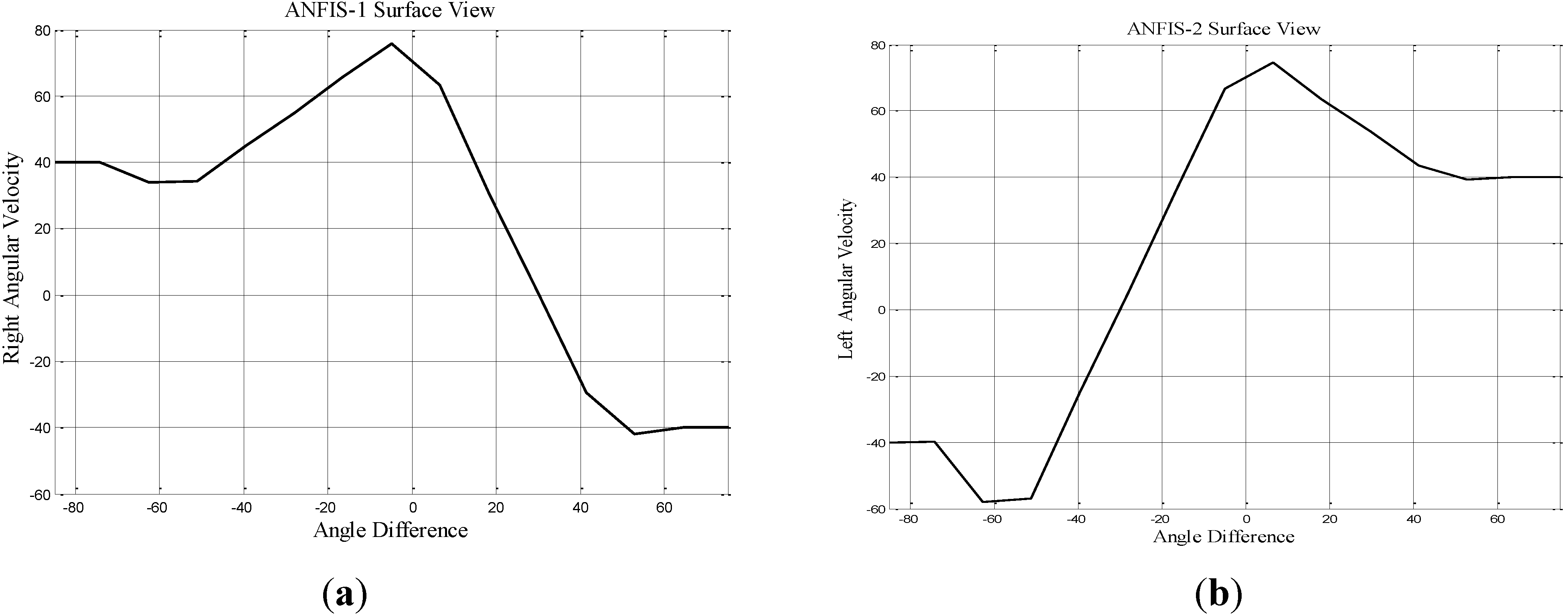
The number of membership functions was chosen for the angle difference input is ten. This number gives a reasonable amount of error as shown in Figure 6. The type of membership function is triangular. The relationship of surface view between angle difference and the output for the first and second ANFIS controllers is illustrated in Figure 8a, b respectively.

Figure 8. The surface view for target reaching ANFIS controller. (a) The first ANFIS controller. (b) The second ANFIS controller.

Figure 8. The surface view for target reaching ANFIS controller. (a) The first ANFIS controller. (b) The second ANFIS controller.

4.3. Obstacle Avoidance ANFIS Controller

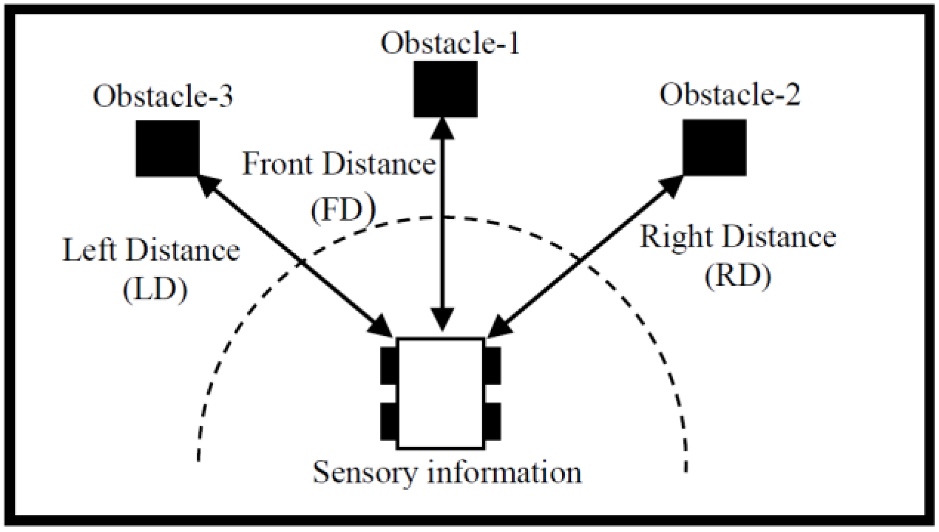
The essential mission of the autonomous ground vehicle is to have a collision free path during the navigation. The other two ANFIS controllers have been implemented to comprise the third and fourth ANFIS controllers. These controllers are utilised to steer the vehicle’s orientation when the vehicle be in the vicinity an obstacle. Each ANFIS has three inputs which are the front, right and left distance and one output which is either the right or left angular velocity. The received sensory information is depicted in Figure 9 which represents the left, right and front distances as inputs for each ANFIS. The output of the third and fourth ANFIS controller is right angular velocity ($w_l$) and left angular velocity ($w_r$) respectively. Each controller regulates the vehicle’s velocities (left or right) depending upon the distances between the obstacles and the current posture of the autonomous ground vehicle.

Figure 9. Schematic diagram for the sensory information.

Figure 9. Schematic diagram for the sensory information.

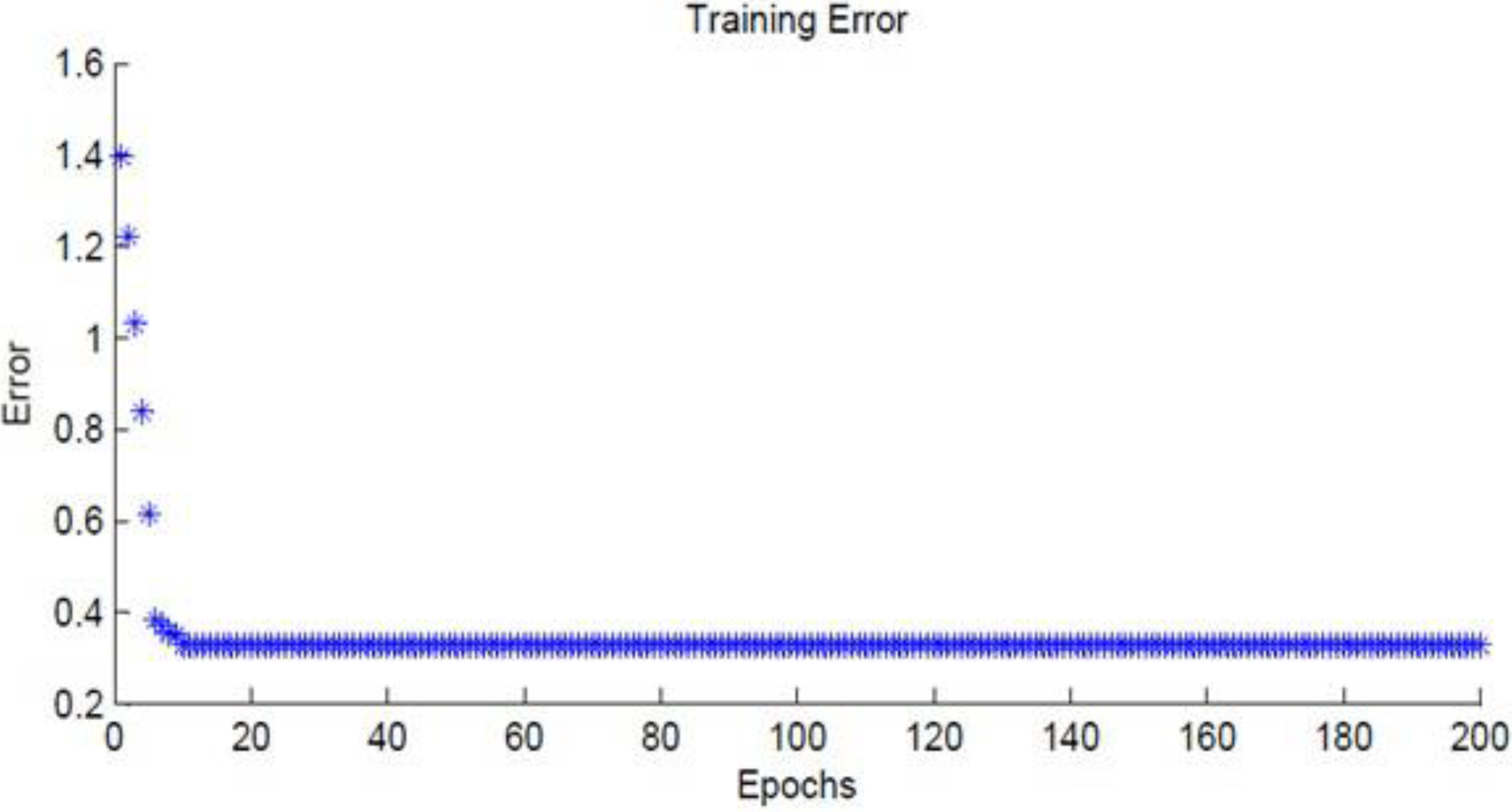
For implementing the obstacle avoidance ANFIS controller, the 21 sets of data range were selected for the training purpose. These training data ranges for inputs and outputs are given in Table 2. This training as mentioned previously adjusts the membership parameters to implement the required model. The ANFIS learning information for predicting the angular velocity for the left and the right wheels are as follows: number of nodes, 286; number of linear parameters, 125; number of nonlinear parameters, 45; total number of parameters, 170; number of fuzzy rules, 125. Training result shows that the average error for predicting angular velocity is 0.329231 rad/s with an epoch number of 200. Again, the relationship between the average error and epoch number is given in Figure 10. 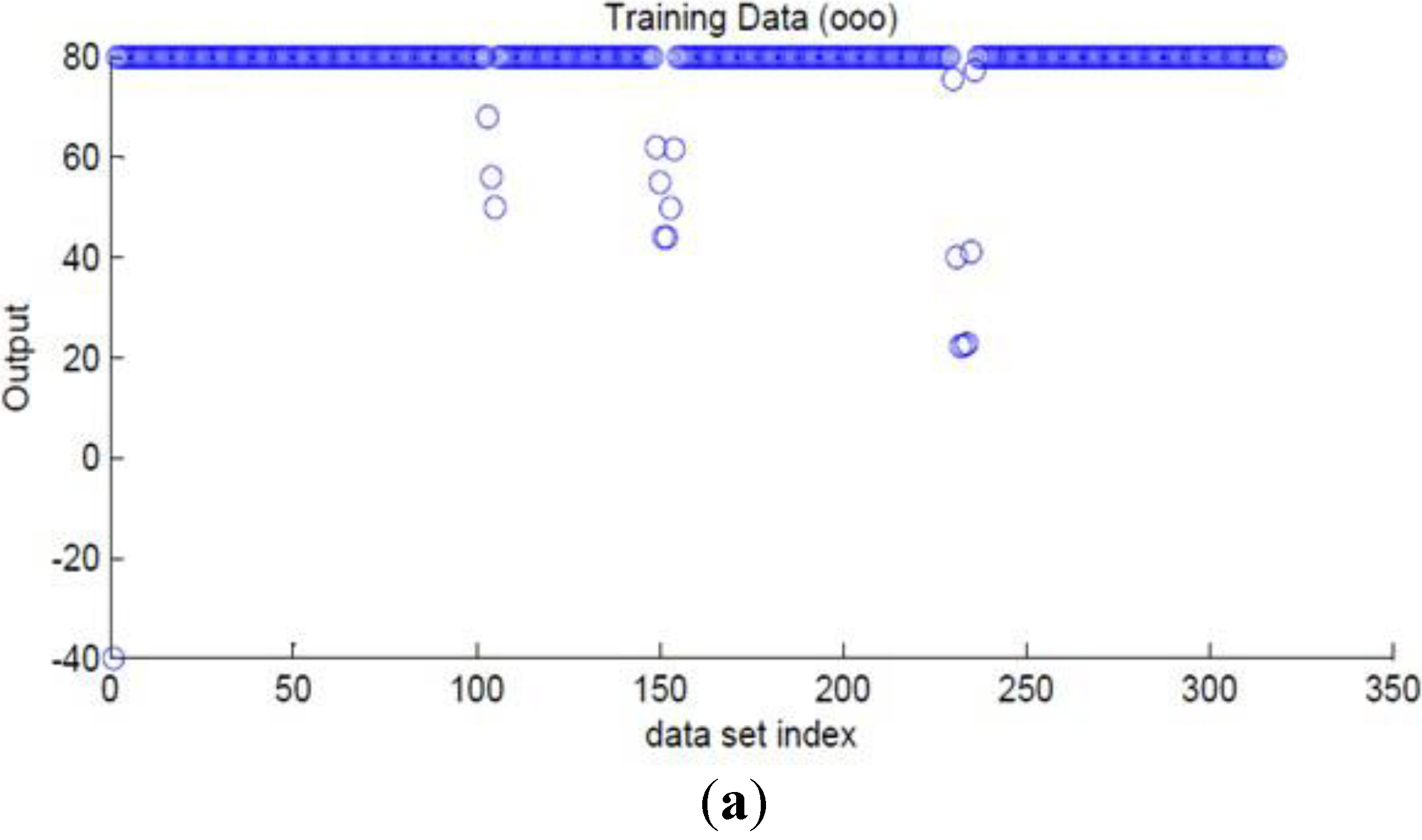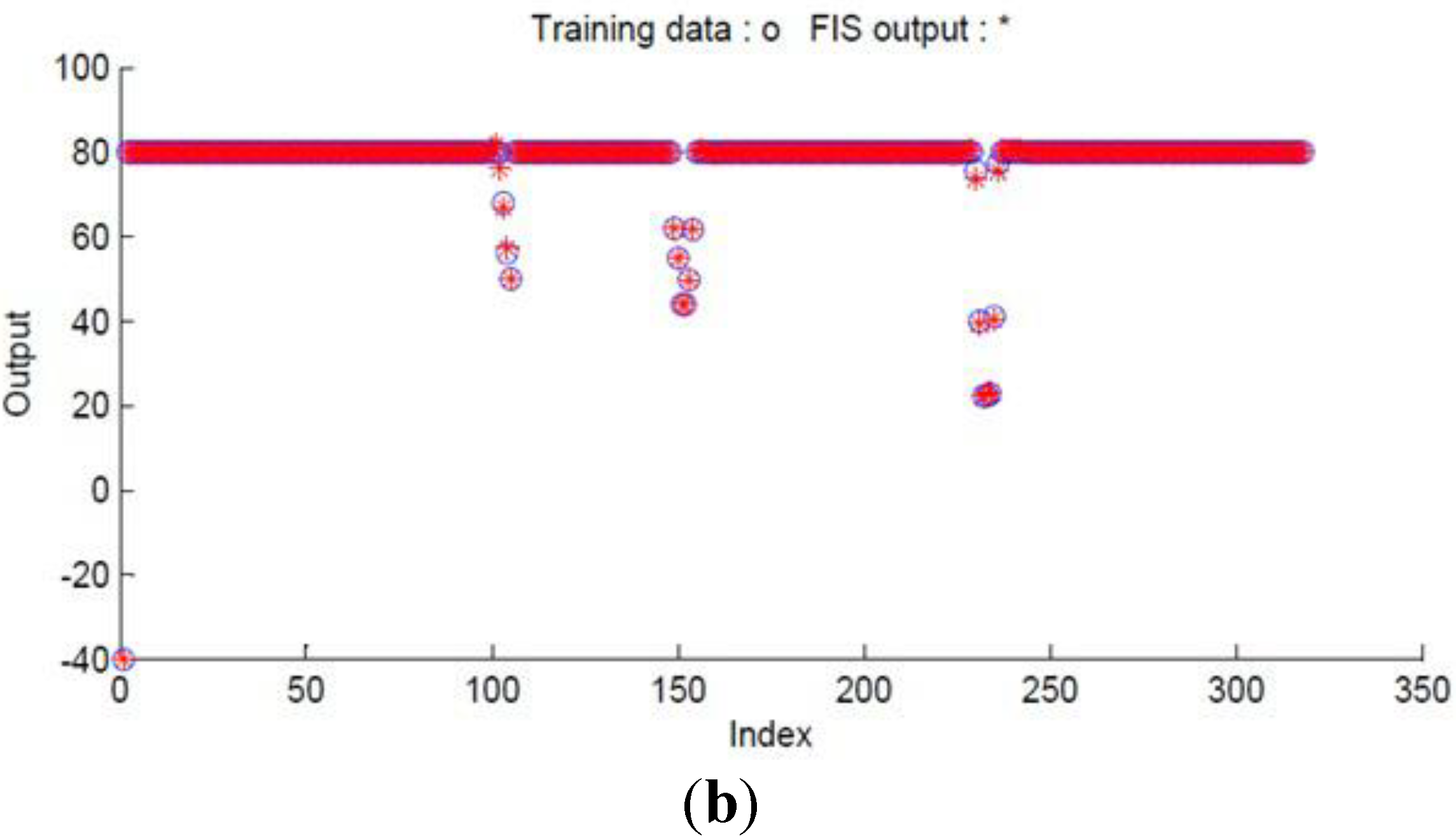Figure 11a, b shows the output training data for obstacle avoidance ANFIS initially before the training and after the training process is completed.

Table 2. Training data of obstacle avoidance ANFIS controller.

Item Number	Front Distance	Right Distance	Left Distance	Right Angular Velocity	Left Angular Velocity
1	0.100	0.100	0.100	−40	−40
2	0.800	0.800	0.800	80	80
3	0.800	0.399	0.800	79.99	79.999
4	0.800	0.339	0.800	67.999	43.999
5	0.800	0.279	0.800	55.999	7.999
6	0.800	0.249	0.800	49.99	−10.006
7	0.547	0.800	0.800	80	80
8	0.4873	0.309	0.800	61.997	25.992
9	0.397	0.279	0.800	54.922	8.351
10	0.4269	0.219	0.800	43.997	−28.008
11	0.515	0.219	0.800	43.967	−28.098
12	0.800	0.249	0.800	49.853	−10.440
13	0.800	0.308	0.800	61.644	24.932
14	0.800	0.800	0.392	75.580	78.526
15	0.800	0.800	0.333	40.013	66.671
16	0.786	0.800	0.303	22.230	60.743
17	0.800	0.800	0.304	22.418	60.806
18	0.800	0.800	0.304	22.803	60.934
19	0.800	0.800	0.335	41.084	67.028
20	0.800	0.800	0.395	77.330	79.110
21	0.800	0.800	0.455	80	80

Table 2. Training data of obstacle avoidance ANFIS controller.

Item Number	Front Distance	Right Distance	Left Distance	Right Angular Velocity	Left Angular Velocity
1	0.100	0.100	0.100	−40	−40
2	0.800	0.800	0.800	80	80
3	0.800	0.399	0.800	79.99	79.999
4	0.800	0.339	0.800	67.999	43.999
5	0.800	0.279	0.800	55.999	7.999
6	0.800	0.249	0.800	49.99	−10.006
7	0.547	0.800	0.800	80	80
8	0.4873	0.309	0.800	61.997	25.992
9	0.397	0.279	0.800	54.922	8.351
10	0.4269	0.219	0.800	43.997	−28.008
11	0.515	0.219	0.800	43.967	−28.098
12	0.800	0.249	0.800	49.853	−10.440
13	0.800	0.308	0.800	61.644	24.932
14	0.800	0.800	0.392	75.580	78.526
15	0.800	0.800	0.333	40.013	66.671
16	0.786	0.800	0.303	22.230	60.743
17	0.800	0.800	0.304	22.418	60.806
18	0.800	0.800	0.304	22.803	60.934
19	0.800	0.800	0.335	41.084	67.028
20	0.800	0.800	0.395	77.330	79.110
21	0.800	0.800	0.455	80	80

Figure 10. Relationship between training error and epoch’s number for obstacle avoidance ANFIS.

Figure 10. Relationship between training error and epoch’s number for obstacle avoidance ANFIS.

Figure 11. The output data for obstacle avoidance ANFIS. (a) The initial data before the training. (b) The matched data after the ANFIS is trained.

Figure 11. The output data for obstacle avoidance ANFIS. (a) The initial data before the training. (b) The matched data after the ANFIS is trained.

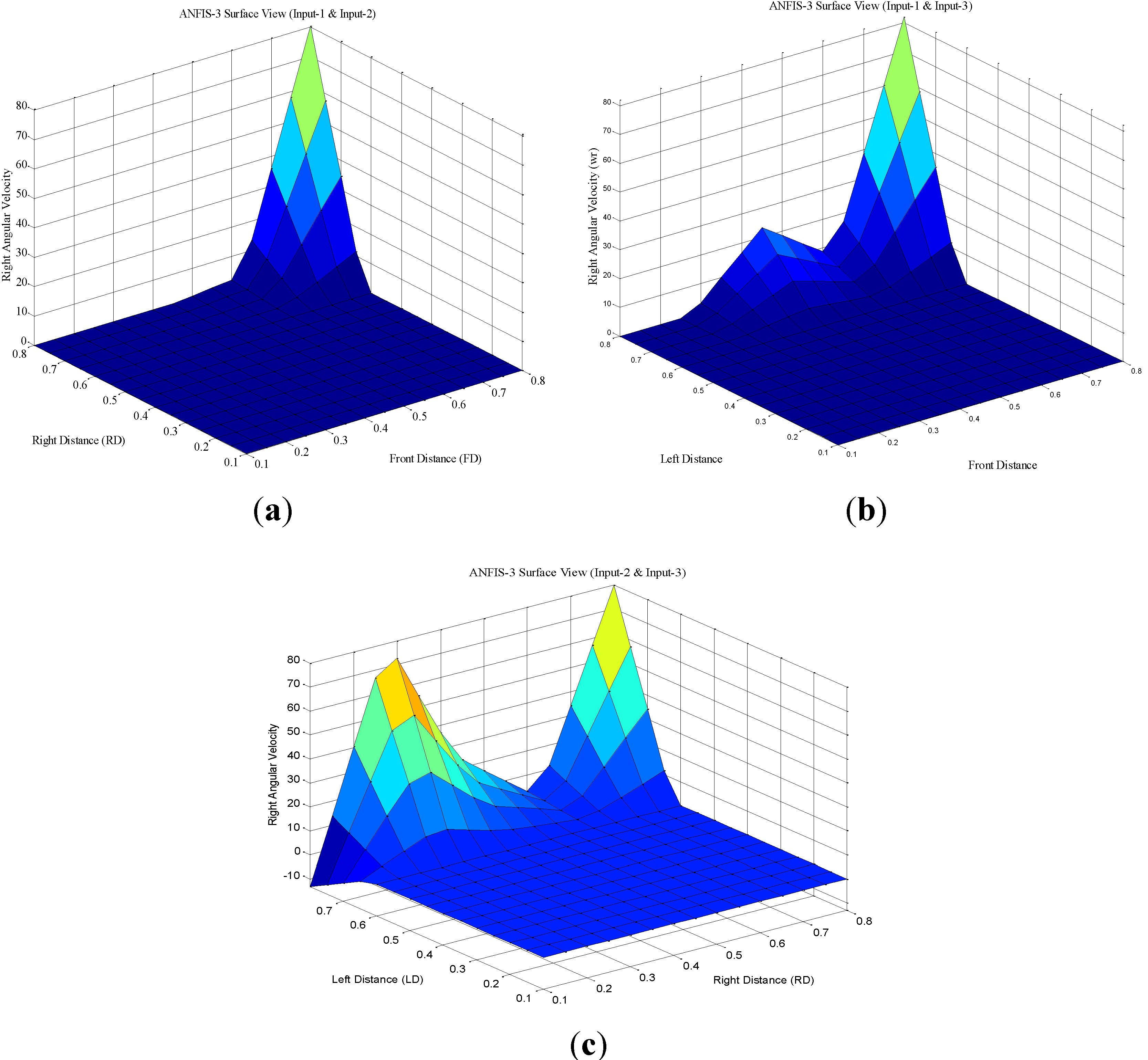
For obstacle avoidance ANFIS controller, the number of membership functions that was chosen for each input is five. Thus, the amount of error was reasonable with this number of membership functions. The type of the membership function is triangular. The surface view between the inputs and the output for the third ANFIS controllers is illustrated in Figure 12.

Figure 12. The surface view for obstacle avoidance ANFIS controller. (a) The surface view between input-1, input-2 and the output. (b) The surface view between input-1, input-3 and the output. (c) The surface view between input-2, input-3 and the output.

Figure 12. The surface view for obstacle avoidance ANFIS controller. (a) The surface view between input-1, input-2 and the output. (b) The surface view between input-1, input-3 and the output. (c) The surface view between input-2, input-3 and the output.

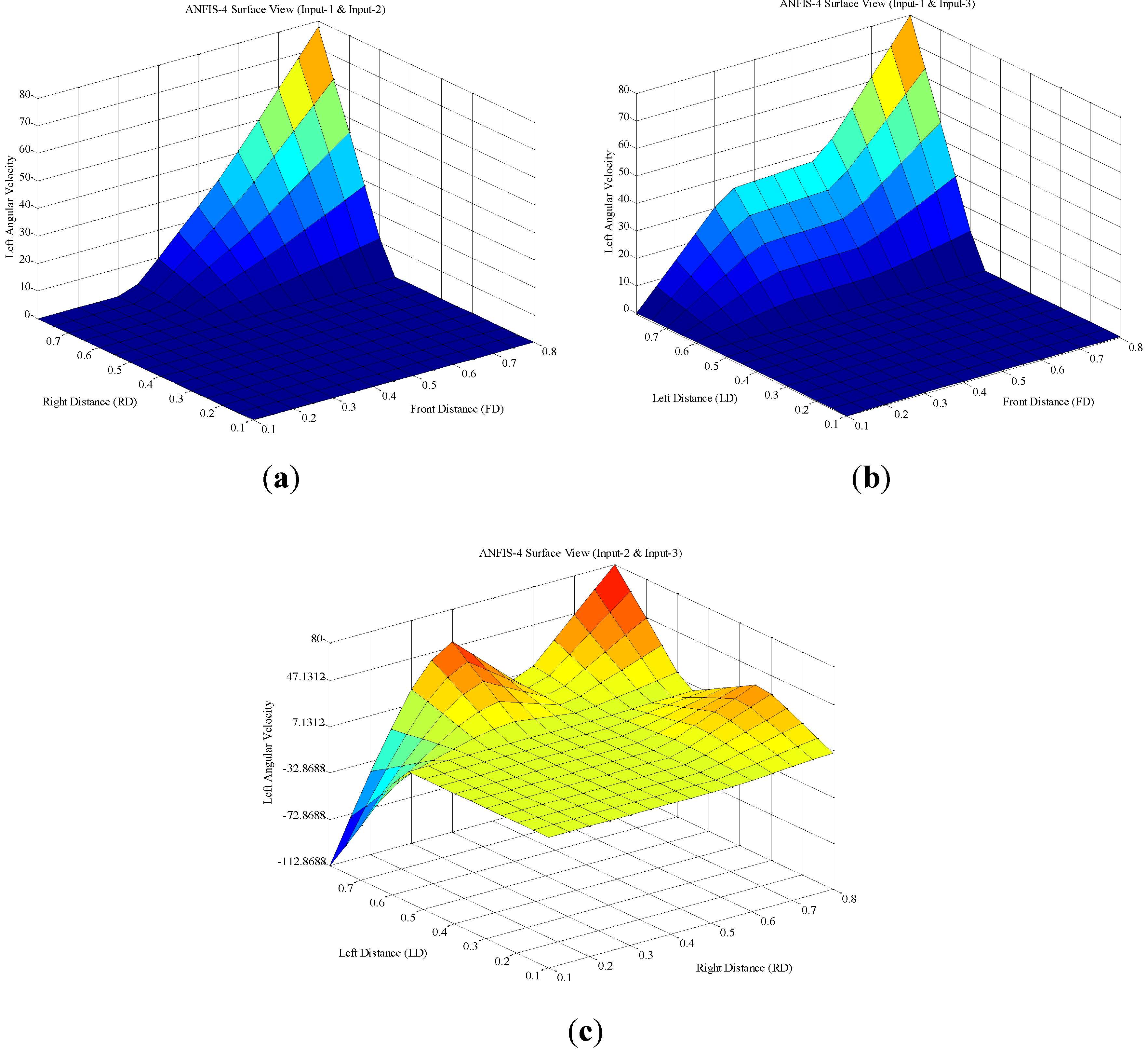
For the fourth obstacle avoidance ANFIS controller, the surface view of the parameters is described in Figure 13.

Figure 13. The surface view for obstacle avoidance ANFIS controller. (a) The surface view between input-1, input-2 and the output. (b) The surface view between input-1, input-3 and the output. (c) The surface view between input-2, input-3 and the output.

Figure 13. The surface view for obstacle avoidance ANFIS controller. (a) The surface view between input-1, input-2 and the output. (b) The surface view between input-1, input-3 and the output. (c) The surface view between input-2, input-3 and the output.

5. Simulation Results

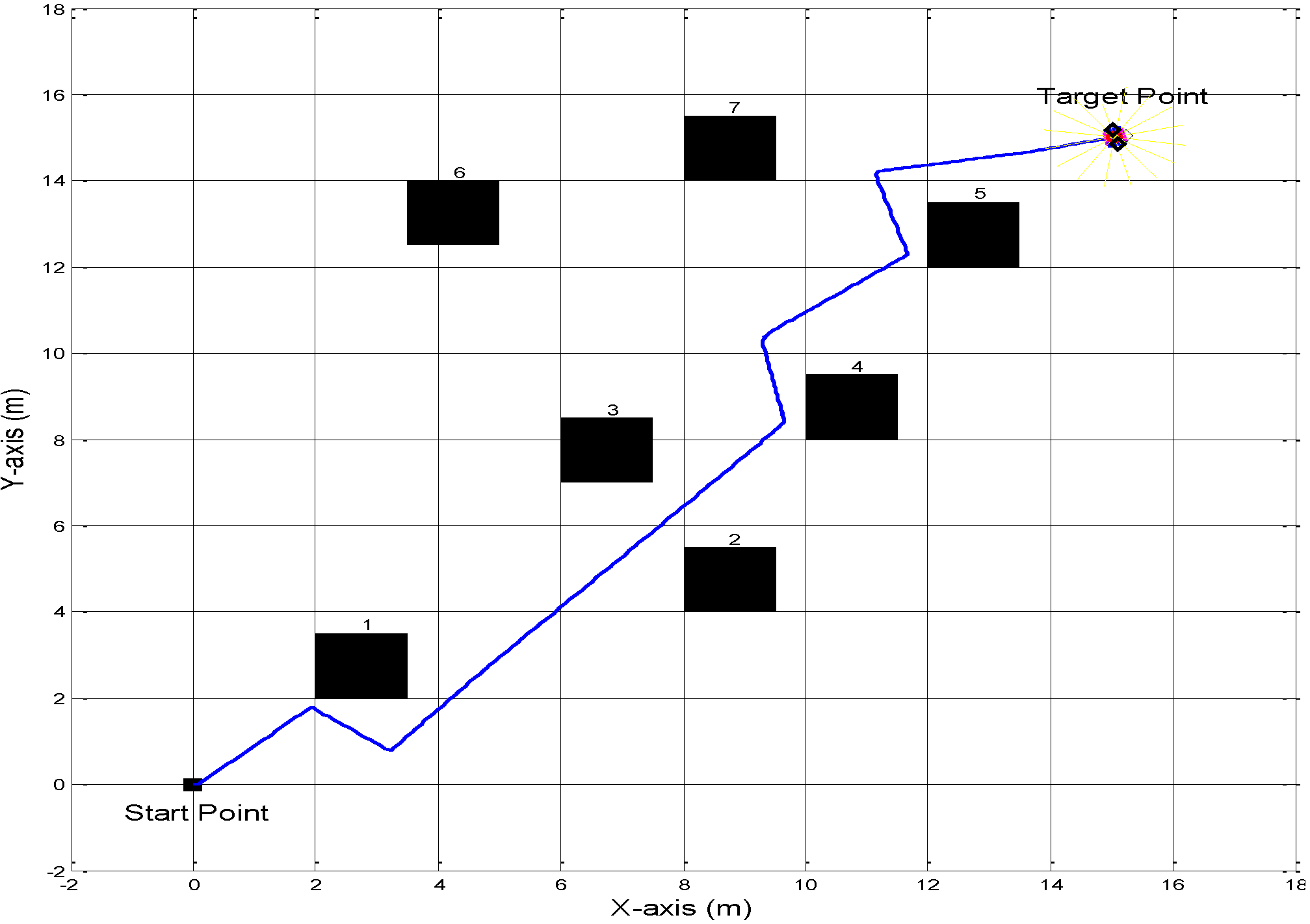
To validate the proposed ANFIS controller, two scenarios have been adopted and carried out in this paper using the MATLAB-SIMULINK environment. In the first scenario, an artificial workspace has been created with seven identical static obstacles that were placed in different positions in the workspace. An initial position and the target point of an autonomous ground vehicle can be set arbitrarily in the workspace. Figure 14 illustrates the workspace for the autonomous vehicle platform filled with seven static obstacles. The workspace dimensions are fixed by four corner points having coordinates (–2, –2), (18, –2), (18, 18), (–2, 18) to combine the workspace grid. The dimensions of the obstacles described by their peripheral vertices are given in Table 3. The Cartesian coordinates of the initial and target points are P_s (0, 0) and P_t (15, 15) respectively.

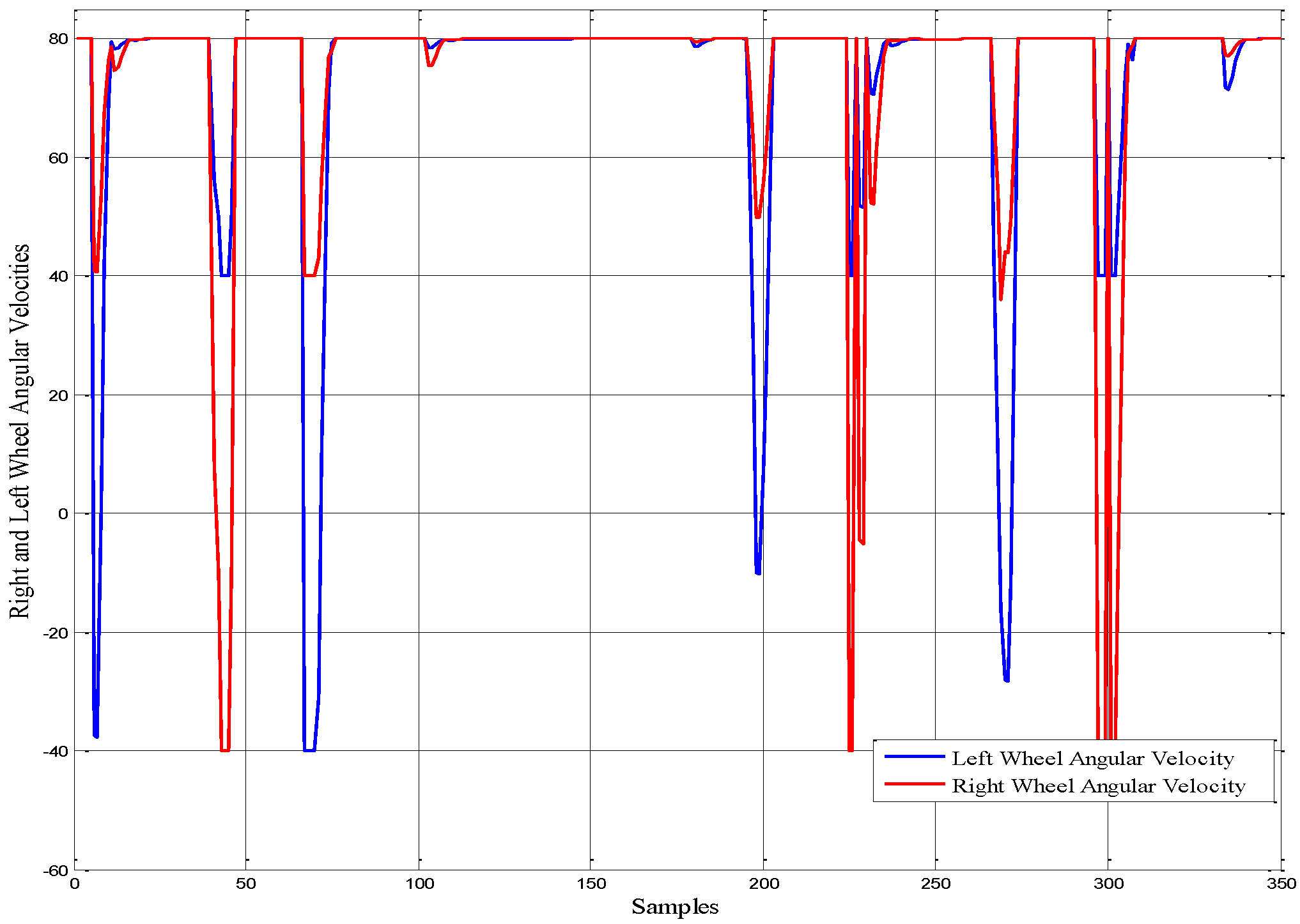
By running the implemented SIMULINK model, the autonomous ground vehicle started moving from a start position towards to the destination position. As can be observed from the Figure 14, the vehicle avoided obstacles successfully and safely. The decision is made to correctly change the vehicle’s direction when it approached the obstacles, and finally, the target is reached. The simulation results of angular velocity for both right and left wheels are shown in Figure 15. 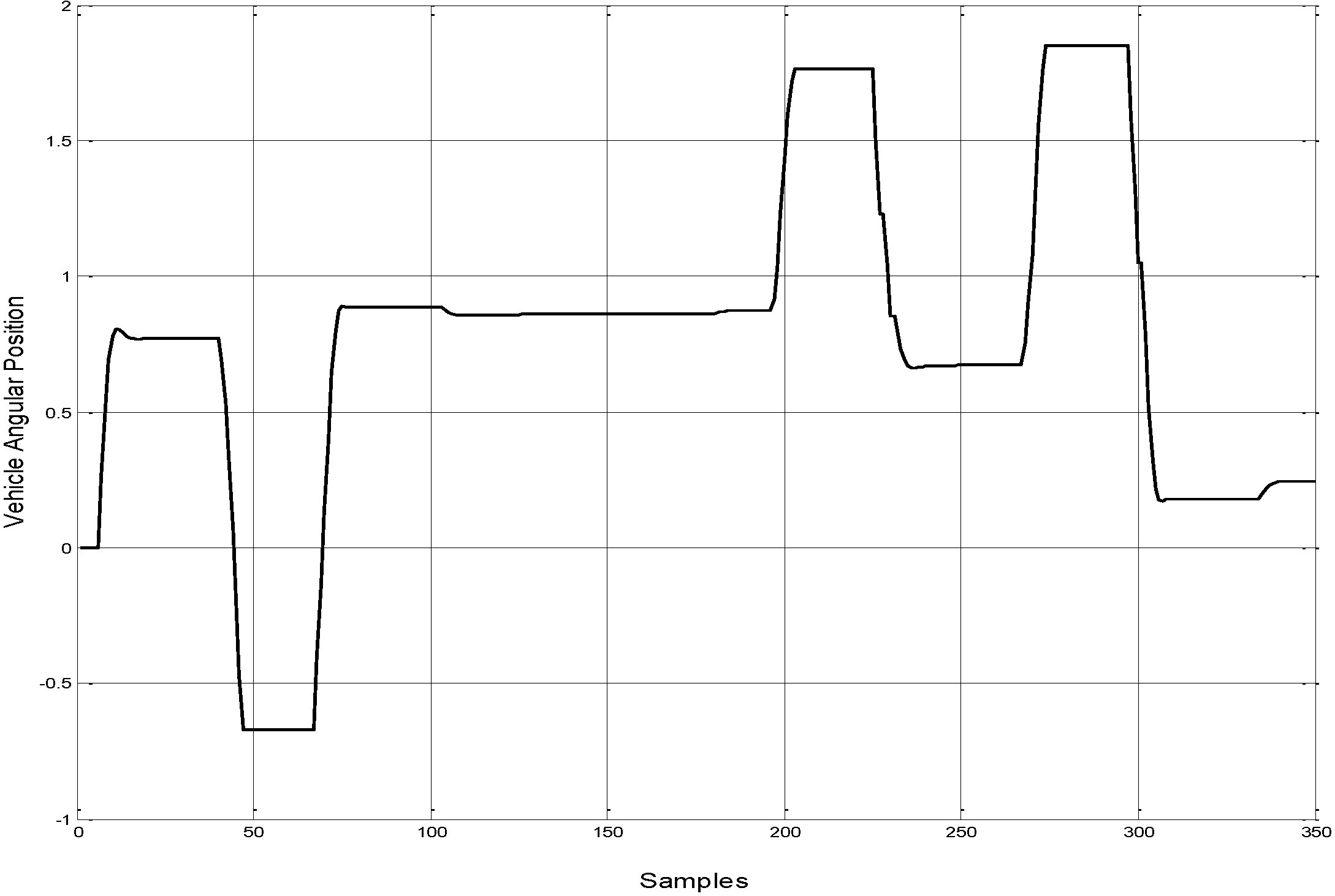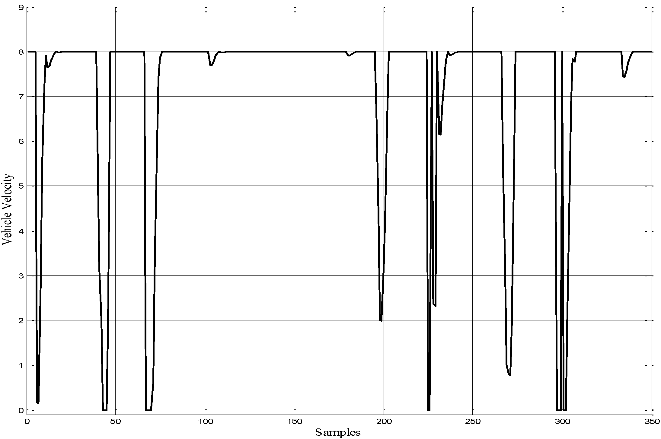Figure 16 represents the angular position of the autonomous ground vehicle. The linear velocity profile is shown in Figure 17. These figures illustrate the changing in the position and velocity of the vehicle when it confronts an obstacle and during the vehicle’s turning.

Table 3. Obstacles description on the workspace grid.

Obstacle No.	Peripheral Vertices Coordinates
1	(2, 2), (2, 3.5), (3.5, 3.5), (3.5, 2)
2	(8, 4), (8, 5.5), (9.5, 5.5), (9.5, 4)
3	(6, 7), (6, 8.5), (7.5, 8.5), (7.5, 7)
4	(10, 8), (10, 9.5), (11.5, 9.5), (11.5, 8)
5	(12, 12), (12, 13.5), (13.5, 13.5), (13.5, 12)
6	(3.5, 12.5), (3.5, 14), (5, 14), (5, 12.5)
7	(8, 14), (8, 15.5), (9.5, 15.5), (9.5, 14)

Table 3. Obstacles description on the workspace grid.

Obstacle No.	Peripheral Vertices Coordinates
1	(2, 2), (2, 3.5), (3.5, 3.5), (3.5, 2)
2	(8, 4), (8, 5.5), (9.5, 5.5), (9.5, 4)
3	(6, 7), (6, 8.5), (7.5, 8.5), (7.5, 7)
4	(10, 8), (10, 9.5), (11.5, 9.5), (11.5, 8)
5	(12, 12), (12, 13.5), (13.5, 13.5), (13.5, 12)
6	(3.5, 12.5), (3.5, 14), (5, 14), (5, 12.5)
7	(8, 14), (8, 15.5), (9.5, 15.5), (9.5, 14)

Figure 14. Navigation platform contains five identical static obstacles.

Figure 14. Navigation platform contains five identical static obstacles.

Figure 15. The angular velocity for both of the right and left wheel angular velocities.

Figure 15. The angular velocity for both of the right and left wheel angular velocities.

Figure 16. The angular position for autonomous ground vehicle.

Figure 16. The angular position for autonomous ground vehicle.

Figure 17. The linear velocity profile for autonomous ground vehicle.

Figure 17. The linear velocity profile for autonomous ground vehicle.

In a more realistic situation, environments might contain obstacles that have different shapes and sizes. In case of increasing the number of obstacles, the frequency of the switching between the obstacle avoidance ANFIS controller and the target reaching ANFIS controller will be increased most the time. This makes the behaviour of the whole system more challenging and the environment more complicated. The performance of the platform was tested in such a case to validate the response of the system in different situations.

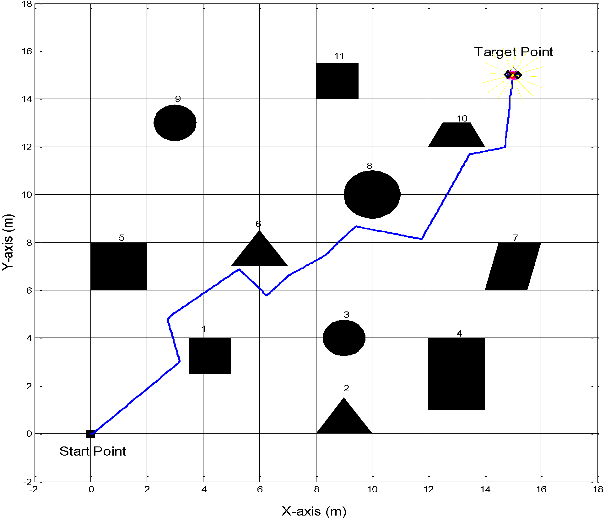
In this second scenario, we considered the vehicle navigating in the case that the obstacles have different sizes and shapes. The dimensions of the obstacles are described by their peripheral vertices are given in Table 4. The number of obstacles was increased to eleven to make a more complex environment. The simulation results showed that the trained obstacle avoidance ANFIS controller made the vehicle traverses all the obstacles in the vehicle’s route by making decisions to change the vehicle’s headings when it approached an obstacle. Decisions are made upon the controllers’ inputs to manipulate the left and right angular velocities. A new feasible trajectory was generated by the autonomous ground vehicle after roving around the obstacles as shown in Figure 18.

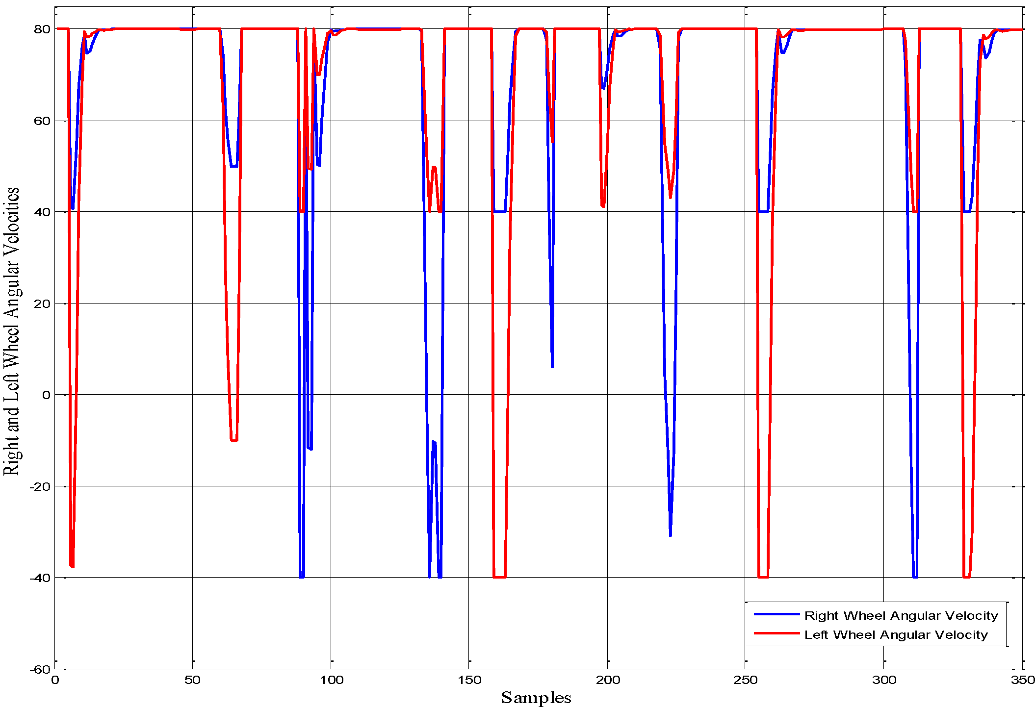
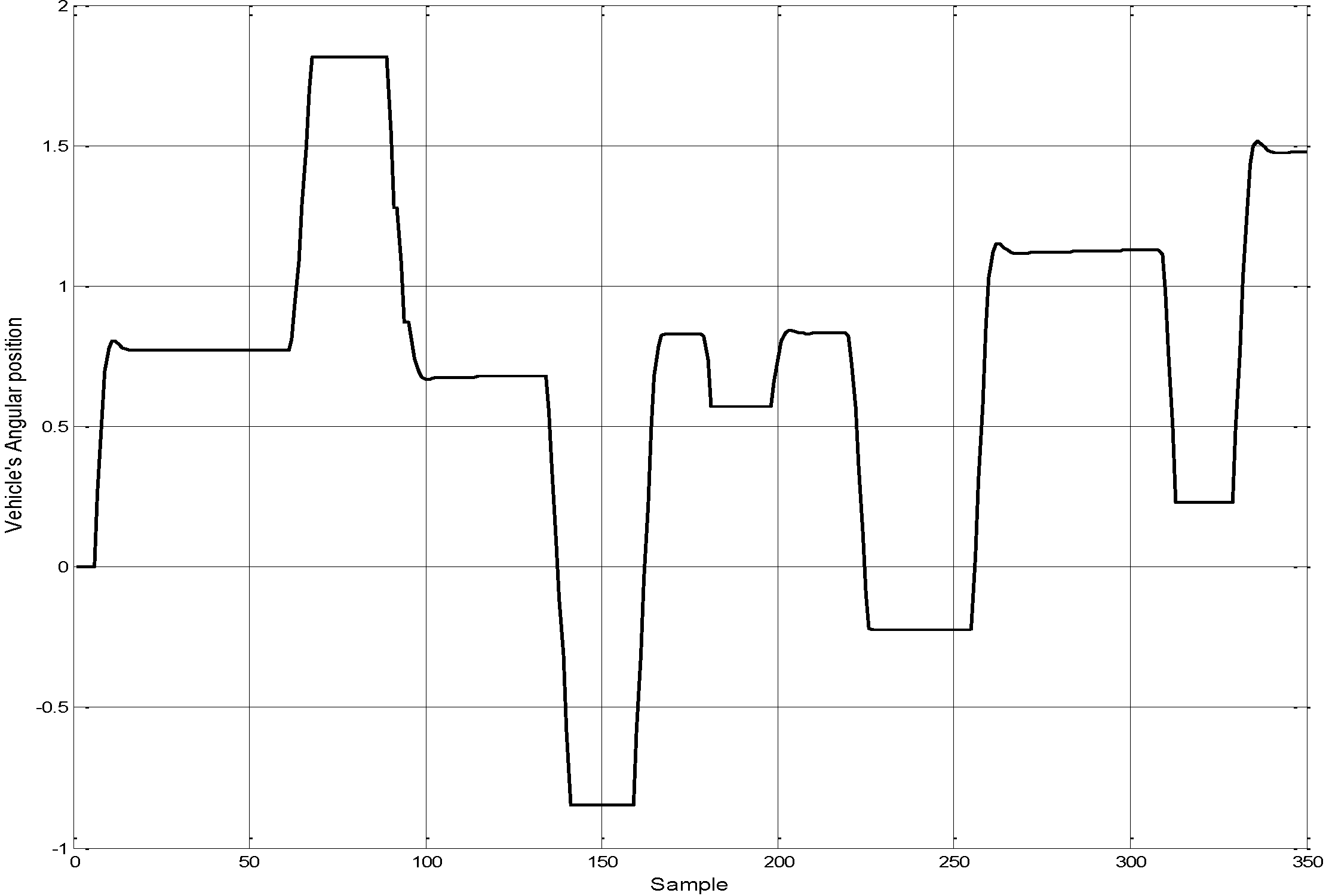
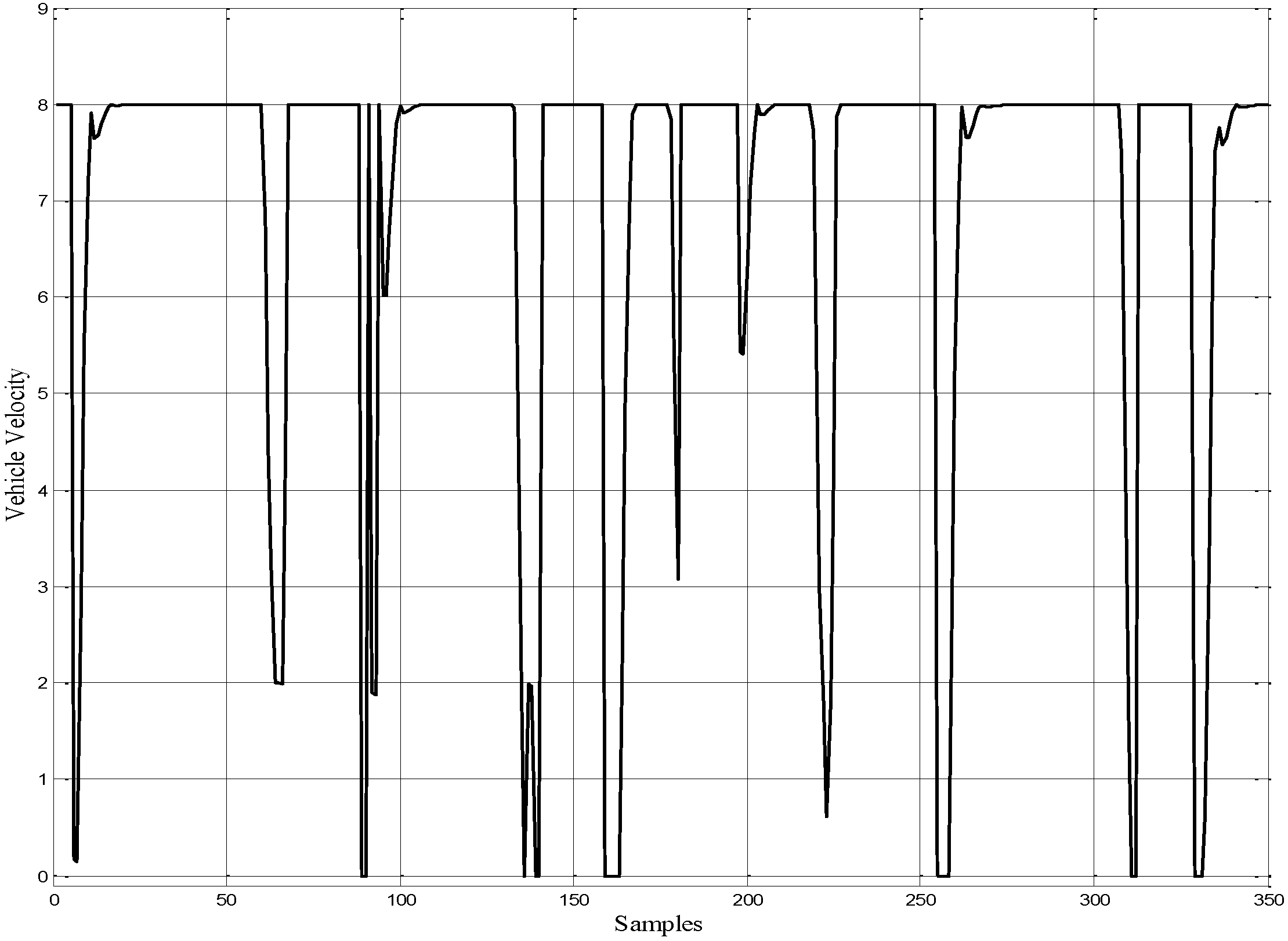
The simulation results of angular velocity for both of right and left wheels are shown in Figure 19. Figure 20 represents the angular position of the autonomous ground vehicle. The linear velocity profile is shown in Figure 21. These figures illustrate the changing in the position and velocity of the vehicle when it wanders around the obstacles.

Table 4. Obstacles description on the workspace grid.

Obstacle No.	Peripheral Vertices Coordinates	Shape Type
1	(3.5, 3.5), (5, 5), (2.5, 4), (4, 2.5)	Square
2	(8, 0), (9, 1.5), (10, 0)	Triangle
3	Centre (9, 4) and Radius = 0.75m	Circle
4	(12, 1), (12, 4), (14, 4), (14, 1)	Rectangle
5	(0, 6), (0, 8), (2, 8), (2, 6)	Square
6	(3.5, 3.5), (5, 5), (15.5, 4)	Triangle
7	(14.5, 8), (16, 8), (15.5, 6), (14, 6)	parallelogram
8	Centre (10, 10) and Radius = 1m	Circle
9	Centre (3, 13) and Radius = 0.75m	Circle
10	(12, 12), (12.5, 5), (13.5, 13), (14, 12)	Trapezoid
11	(8, 14), (8, 15.5), (9.5, 15.5), (9.5, 14)	Square

Table 4. Obstacles description on the workspace grid.

Obstacle No.	Peripheral Vertices Coordinates	Shape Type
1	(3.5, 3.5), (5, 5), (2.5, 4), (4, 2.5)	Square
2	(8, 0), (9, 1.5), (10, 0)	Triangle
3	Centre (9, 4) and Radius = 0.75m	Circle
4	(12, 1), (12, 4), (14, 4), (14, 1)	Rectangle
5	(0, 6), (0, 8), (2, 8), (2, 6)	Square
6	(3.5, 3.5), (5, 5), (15.5, 4)	Triangle
7	(14.5, 8), (16, 8), (15.5, 6), (14, 6)	parallelogram
8	Centre (10, 10) and Radius = 1m	Circle
9	Centre (3, 13) and Radius = 0.75m	Circle
10	(12, 12), (12.5, 5), (13.5, 13), (14, 12)	Trapezoid
11	(8, 14), (8, 15.5), (9.5, 15.5), (9.5, 14)	Square

Figure 18. Navigation platform contains eleven static obstacles with different sizes and shapes.

Figure 18. Navigation platform contains eleven static obstacles with different sizes and shapes.

Figure 19. The angular velocity for both of the right and left wheel angular velocities.

Figure 19. The angular velocity for both of the right and left wheel angular velocities.

Figure 20. The angular position for autonomous ground vehicle.

Figure 20. The angular position for autonomous ground vehicle.

Figure 21. The linear velocity profile for autonomous ground vehicle.

Figure 21. The linear velocity profile for autonomous ground vehicle.

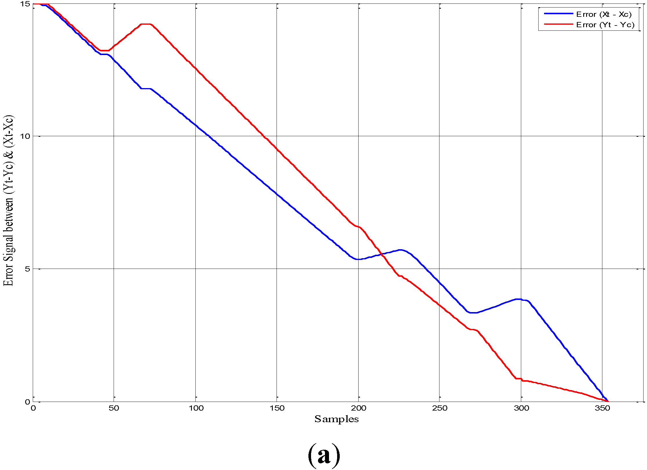
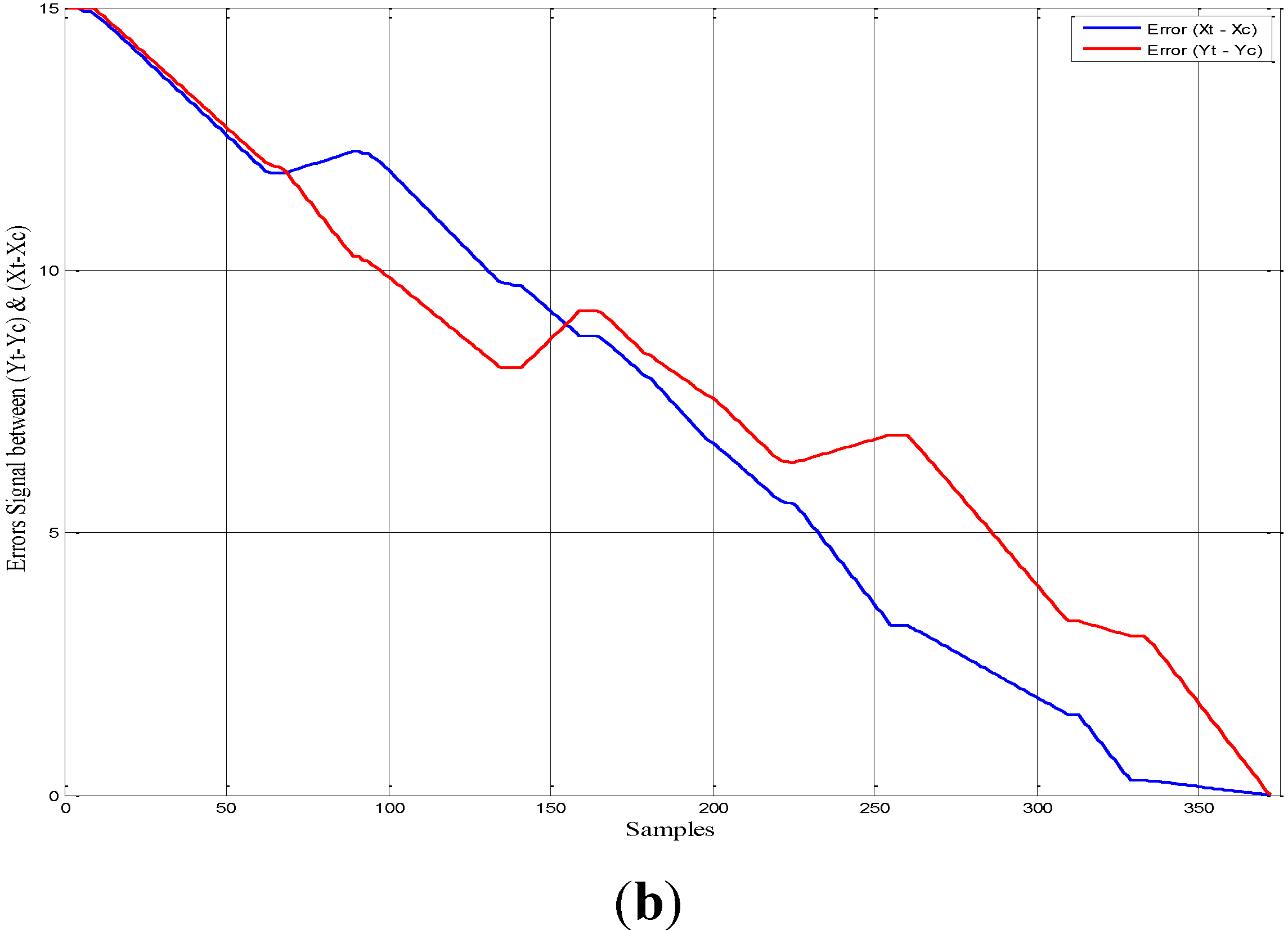
Figure 22. The Error rate between the target point and vehicle’s actual point. (a) First scenario. (b) Second scenario.

Figure 22. The Error rate between the target point and vehicle’s actual point. (a) First scenario. (b) Second scenario.

The error signals for both of x and y coordinates between the target point (x_t = 15, y_t = 15) and the vehicle’s actual points during the navigation was obtained. These signals of the autonomous ground vehicle for the first and second scenarios are shown in Figure 22a,b respectively. The results show the behaviour of the vehicle as it reached its destination. Before the vehicle started moving the error rate was maximum and when the vehicle arrived at its target the error rate became zero.

6. Conclusion

In this paper, an adaptive neuro-fuzzy inference system has been implemented to control the angular velocities of the wheels of an autonomous ground vehicle. These velocities guide the vehicle safely to reach the destination in a static environment without colliding with obstacles presented on its way. The proposed system utilises four ANFIS controllers. Firstly, two controllers for the target reaching which to ensure that the vehicle reaches its destination point; Secondly, two controllers for guiding the vehicle to avoid the collision with obstacles. In these four controllers, the right and left angular velocities will derive the vehicle’s heading during the navigation.

The validation of the proposed method has been demonstrated by considering two scenarios; firstly, seven identical static obstacles are placed randomly with the workspace; secondly, eleven obstacles have different sizes and shapes. In case of reducing obstacle numbers significantly, the obstacle avoidance ANFIS controller did not activate until the vehicle confronted an obstacle. Therefore, the target reaching ANFIS controller was active most of the time. This case will be similar in the situation if a path is free of obstacles so the vehicle will take straight line that connects between both start and target points.

In contrast, in multiple obstacles simulation, the obstacle avoidance ANFIS controller was activated frequently in order to avoid obstacles. After each avoiding point the vehicle switched to the target reaching ANFIS controller. In both considered scenarios, the autonomous ground vehicle was capable of avoiding obstacles safely and reaching the target with a feasible and smooth online generated path between the initial and the target points. The simulation experiments have been conducted using MATLAB-Simulink software package.

In the future, the proposed ANFIS control strategy will be implemented in a real AGV to further verify its feasibility and performance.