2. Types of Illumination Invariance
In this section, we introduce different types of invariance against shift and scaling of intensities within an image region (in the case of min-warping: a column of a panoramic image). This allows us to classify the distance measures introduced in
Section 3 accordingly. For simplicity, the following discussion assumes a one-dimensional, continuous representation of intensities
and
in two image regions. A distance measure
computes some (non-negative) integral over these intensity functions. We assume that a perfect match is indicated by a distance measure of zero,
i.e.,
.
The methods investigated here establish tolerance against intensity shifts (additive changes) or against intensity scaling (multiplicative changes) over the entire region. In addition, as will be discussed below (
Section 6), those distance measures which work on edge-filtered images appear to achieve some kind of local invariance within each image region.
This work deals with two types of
invariance against intensity scaling,
i.e., against multiplicative changes in intensity. The first type we call
weak scale invariance which is achieved if the distance measure exhibits the property
This means that for an arbitrary intensity scaling of an intensity function by a factor
c, the distance measure indicates a perfect match with the original intensity function. The second type,
strong scale invariance, includes weak scale invariance but in addition ensures that
i.e., scaling of one intensity function has no effect on the distance to the other intensity function. This is the stronger type of scale invariance since it not only guarantees that the match of an image region
with itself is invariant to scaling, but also that the distance to a
different image region is unaffected by scaling. We expect that measures with strong scale invariance will perform better than those with weak scale invariance.
Every distance measure can be made
invariant against intensity shifts,
i.e., against offsets in intensity. In this work, shift invariance is accomplished by subtracting the mean value or by performing a first-order differentiation before applying the distance measure, or both. If one of the vectors is shifted by an offset
c, the distance measure is not affected if the mean is subtracted beforehand,
or if the distance measure is applied to edge-filtered images,
It is clear that if two intensity functions are scaled versions of each other,
i.e.,
, then their derivatives will also be scaled versions of each other
as will be their zero-mean versions,
and the zero mean versions of the derivatives,
where
and
are the means of the derivatives. Obviously the methods used to introduce additional shift invariance have no effect on scale relationships.
While subtracting the mean removes intensity shifts affecting the entire image region, a first-order differentiation also removes local intensity shifts in sub-regions of constant intensity; only the edge slope between regions of constant intensity is affected. We suppose that this introduces local illumination tolerance (see discussion in
Section 6).
3. Distance Measures
In the following subsections we introduce the different distance measures explored in this work. We start with the tunable sum of squared differences since it includes the Euclidean distance—which was originally used by min-warping—as a special case (
Section 3.1). A zero-mean version is introduced in
Section 3.2. Normalization of the illumination-invariant portion leads to the well-known normalized cross-correlation (
Section 3.3). In its tunable form, this measure is combined with the absolute difference of the sum of the intensities; the same illumination-sensitive term is used in all following methods. A zero-mean version of normalized cross-correlation is introduced in
Section 3.4. In
Section 3.5 we present distance measures where normalized cross-correlation and its zero-mean version are applied to edge-filtered image columns, since also the novel correlation-like measures introduced in this work include an edge filter. Again, tunable versions are defined. We then describe the two novel correlation-like measures introduced in this work, “sequential correlation” (
Section 3.6) and its approximated version (
Section 3.7), both also available as tunable versions.
In the following we make predictions on the effects of the different distance measures on the performance of min-warping. As performance criterion, we always assume the home vector error as described in
Section 4.3.
3.1. Tunable Sum of Squared Differences (TSSD)
In its original form, our visual navigation method “min-warping” computed the Euclidean distance (the square root of the “sum of squared differences”, SSD) between two image columns. The indoor image databases used in the evaluation of the method [
20] were collected under constant or moderately varying illumination (mostly caused by changing cloud cover over the day), but not under extreme variations in illumination (like changes between day and night or between natural and artificial illumination). Camera-gain control and histogram equalization were applied to reduce the impact of illumination changes (note that, even under constant illumination, these steps introduce moderate intensity changes as well). Under these conditions, SSD produced robust navigation performance.
Unsurprisingly, as the experiments below will demonstrate, the performance of SSD breaks down under stronger changes in illumination. We therefore first attempt to develop a distance measure which is related to SSD—keeping the good performance under the above-mentioned mild conditions—but which is at the same time tolerant against changes in illumination. For this we assume that changes have a multiplicative effect on the intensities (with intensities being encoded by non-negative values). A distance measure invariant against multiplicative changes should rate the distance between two intensity vectors as minimal (zero) if one is a scaled version of the other.
As shown in
Section 2, additional tolerance against
additive changes can be achieved by subtracting mean intensities from the intensity vectors. However, it is unclear how this will affect the performance of min-warping: First, invariance against scaling and shift are partly exchangeable—in noisy images it may be difficult to distinguish between moderate scaling and shift. Second, introducing too much tolerance may lead to mismatches. We will explore the influence of double invariance in the experiments.
Applying an illumination-invariant distance measure alone may, however, falsely indicate matches for intensity vectors which are representing different features in the environment and markedly differ in their overall intensity but which nevertheless are scaled (or shifted) versions of each other. While this may occur only rarely in structured image regions, indoor environments often contain uniformly colored walls, curtains, or furniture which can only be distinguished by their overall intensity. Since min-warping does not preselect features (e.g., high-variance regions around corners), ignoring these overall intensity differences may discard information valuable for visual homing. The illumination-invariant measure should therefore be combined with a second, illumination-sensitive measure expressing the difference in the overall intensities of the two image columns. Depending on a weight factor, the influence of both measures can be tuned. We expect that there will be an optimal, intermediate weight factor with respect to the navigation performance.
In the following derivations, the vectors encoding the intensities of the two image columns are denoted by
and
, both of dimension
n, with
and
. We start with the derivation of the illumination-invariant part of the measure. We suggest a novel form of the “parametric sum of squared differences” (PSSD, see e.g., [
64,
65]) where the scale parameter
is split and distributed to both vectors such that the resulting measure is inversion-symmetric (
i.e., if
and
are exchanged, the scale factor is inverted but the distance stays the same):
We determine the optimal value
where the distance
becomes minimal. It is straightforward to show that the optimal scale factor is
If we insert
into Equation (
1) we obtain
We see from the second Equation (
4) that the measure is closely related to the widely used normalized cross-correlation NCC (see e.g., [
60,
63,
64,
65]), but leaves out the normalization.
becomes zero if and only if one intensity vector is a scaled version of the other,
thus the measure exhibits
weak scale invariance; see
Section 2. Since
the measure does not exhibit strong scale invariance, though. Since the measure was derived from a quadratic term, it is non-negative. This property is also directly visible from Equation (
3) by applying the Cauchy-Schwarz inequality.
For the comparison of the overall intensities we use the squared difference of the length (SDL):
The combined distance measure, which we call “tunable sum of squared differences” (TSSD), is
where
w is a weight factor from the interval
. For
, TSSD only contains the illumination-invariant portion; for
, it only considers overall intensity differences.
Interestingly, the SSD
is obtained as the special case
of the TSSD in Equation (
5) (up to a constant factor),
The SSD measure can therefore be interpreted as a 2:1 mixture of the fully illumination-invariant PSSD measure and the SDL measure expressing the difference in overall intensities. Reducing the weight w below emphasizes the illumination-invariant portion, and we expect an optimal performance of our navigation method in this range. Note that this quantitative interpretation of the weight is only possible for TSSD, not for the other tunable distance measures presented below.
In our implementation of min-warping, we use
as distance measure to stay close to the Euclidean distance used before (the square root is applied before column distances are summed over the entire image, with the sum indicating the overall match; see [
20]).
3.2. Tunable Zero-Mean Sum of Squared Differences (TZSSD)
We also implemented a zero-mean version of TSSD, called TZSSD in the following. Here the illumination-invariant portion
is computed for two zero-mean intensity vectors,
where
and
are the means of the vectors
and
, respectively, and
. Since most parts of our implementation of PSSD use
unsigned integers, we do not subtract the mean in the beginning, but correct for the mean at later stages in the computation (which is possible by expanding the expression for the zero-mean vectors).
The illumination-sensitive portion is determined from the original intensity vectors, not from the zero-mean versions (since it would otherwise be zero). For this and all following tunable measures we use the absolute difference of sums (ADS) as the illumination-sensitive portion
This measure is somewhat easier to compute in an SSE implementation (see
Section 4.1) since it doesn’t include multiplications and since we don’t have to take the square root. Moreover, the experiments show that this measure alone (
) works as well as SDL (see
Section 5.2). The factor
κ results from factors in our integer-based implementation; for input images with pixel range
it is
for all correlation-type measures and
for TZSSD.
The TZSSD measure can be written as
A subtraction of the mean makes the PSSD measure invariant to shifts in illumination (see
Section 2). Since PSSD already exhibits (weak) invariance against multiplicative changes in illumination, the resulting measure is invariant against both scaling and shift. We expect a loss of performance compared to TSSD due to an increased portion of false-positive matches as discussed above.
3.3. Tunable Normalized Cross-Correlation (TNCC)
We already saw that PSSD is related to normalized cross-correlation NCC, except for the missing normalization; see Equation (
4). In fact, we could derive a form of NCC — here called NCC+ since it only returns positive values from the interval
— from the distance measure
We obtain the same optimal value for gamma as in Equation (
2), and by inserting the optimal gamma into Equation (
6) we get
where the original NCC measure (see e.g., [
63]) is underbraced. Alternatively — and this makes the principle underlying this measure more clear —, NCC+ can be written as
where obviously the scaling between the two vectors is eliminated by normalizing them before computing their SSD distance. While normalized cross-correlation can be interpreted as a distance measure, it can also be seen as a transformation (normalization) accomplishing scale invariance followed by a matching using a simpler distance measure, here SSD (for further interpretations of the correlation coefficient, see [
75]). NCC+ exhibits
strong scale invariance since
thus we expect a better performance than the PSSD measures.
However, as pointed out by [
76], normalization in the presence of noise leads to erroneous estimates for small vectors which may negatively affect the performance. In most feature-matching methods (review: [
4]), features to be matched are only extracted at selected key points where the intensities in the neighborhood vary strongly (often corners or scale-space extrema are detected). Normalization is unproblematic in this context as the denominator is far from zero. Min-warping, in contrast, matches
all image columns without any selection, thus also image columns with low intensity will be processed by the distance measure. Since the denominator of NCC approaches zero in regions of low intensity, numerical problems may occur and image noise is amplified, adding to the difficulty to make predictions of the performance of NCC+. In our integer-based implementation (using 16 bit unsigned words), we add 1 to the integer denominator to avoid division by zero (if one of the vectors has zero length, a value of
is obtained).
For the tunable version, we combine NCC+ with the absolute difference of sums:
3.4. Tunable Zero-Mean NCC (TZNCC)
We also implemented a zero-mean version of NCC+,
The tunable form is called TZNCC,
Here the problem of small denominators is even more severe since it occurs not only for vectors with low intensities, but for all vectors with low variance. This may lead to a performance loss in addition to the problems we expect as a results of the double invariance (see above).
3.5. Tunable NCC on Edge Images (TENCC, TEZNCC)
Edge filtering is integral part of our novel “sequential correlation” methods (
Section 3.6 and
Section 3.7). For comparison, edge filtering should also be considered as preprocessing step for the standard correlation method (NCC). Since min-warping uses image columns as features, a first-order vertical edge detector is applied (subtraction of the intensities of subsequent, neighboring pixels):
We introduce abbreviations for the illumination-invariant terms,
the bottom one being the zero-mean version, and define the tunable measures TENCC and TZENCC:
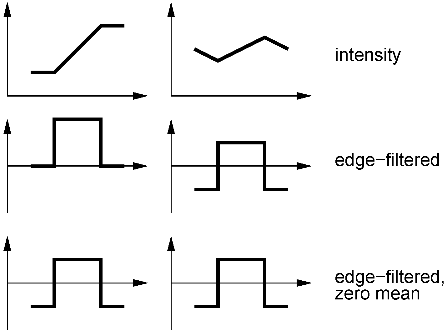
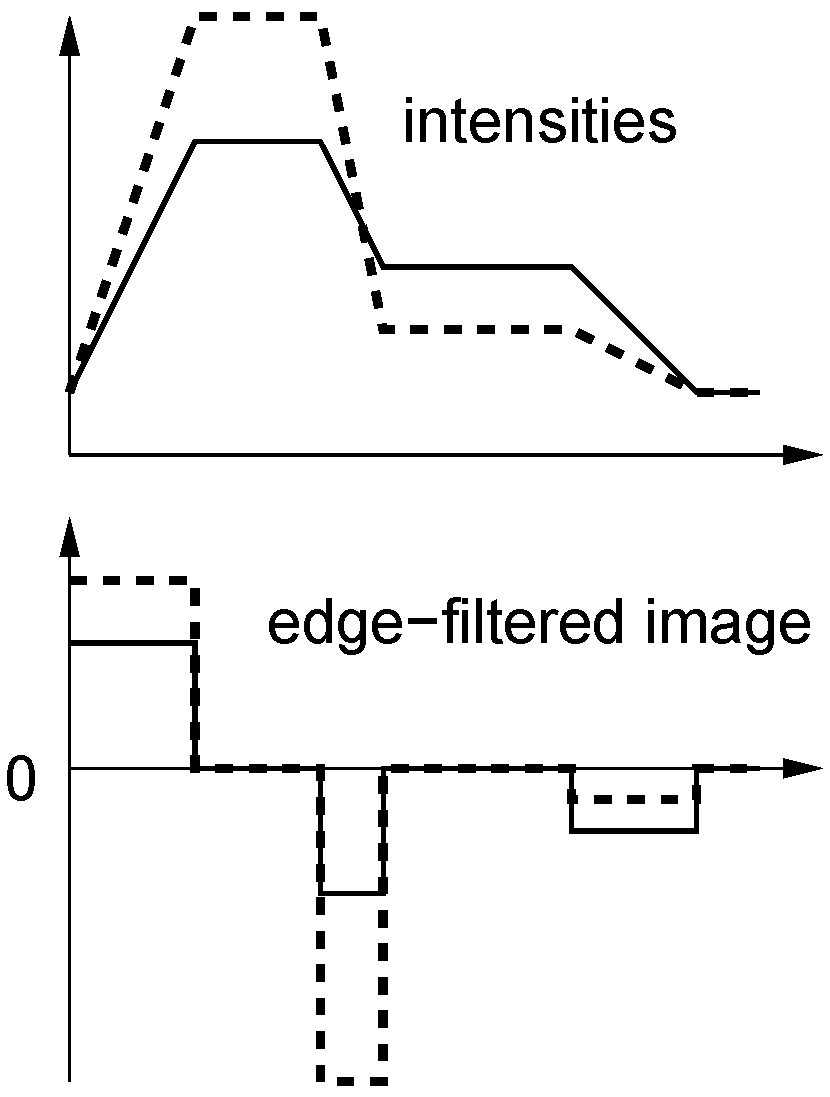
Figure 6.
Two identical edge-filtered, zero-mean columns can correspond to widely differing intensity columns.
Figure 6.
Two identical edge-filtered, zero-mean columns can correspond to widely differing intensity columns.
The effect of subtracting the mean is difficult to predict. On the one hand, a column of
n intensity differences will already have a small mean with a maximal absolute value of
if the intensities come from the interval
, so any effect should be small. On the other hand, very different intensity vectors can have the same zero-mean edge-filtered version, so there is the danger of mismatches; see
Figure 6. We therefore expect a small performance loss if the mean is subtracted.
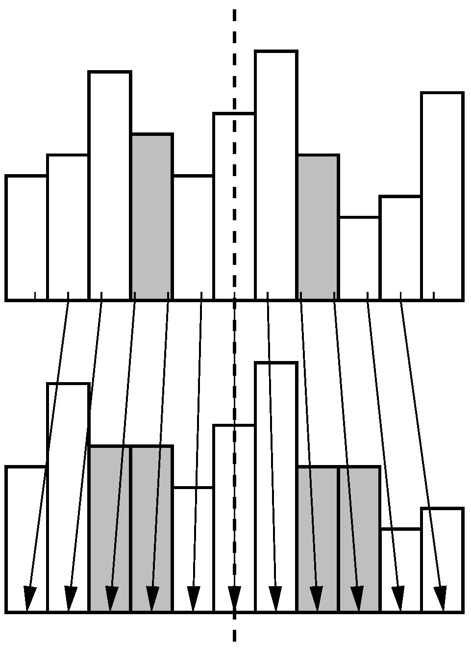
Figure 7.
Magnification around the horizon (dashed line) using nearest neighbor interpolation leads to duplicated pixels (gray bars). Intensities in the original (top) and magnified 1D image column (bottom) are shown as bars in order to visualize the nearest-neighbor selection. Arrows indicate the pixel assignment.
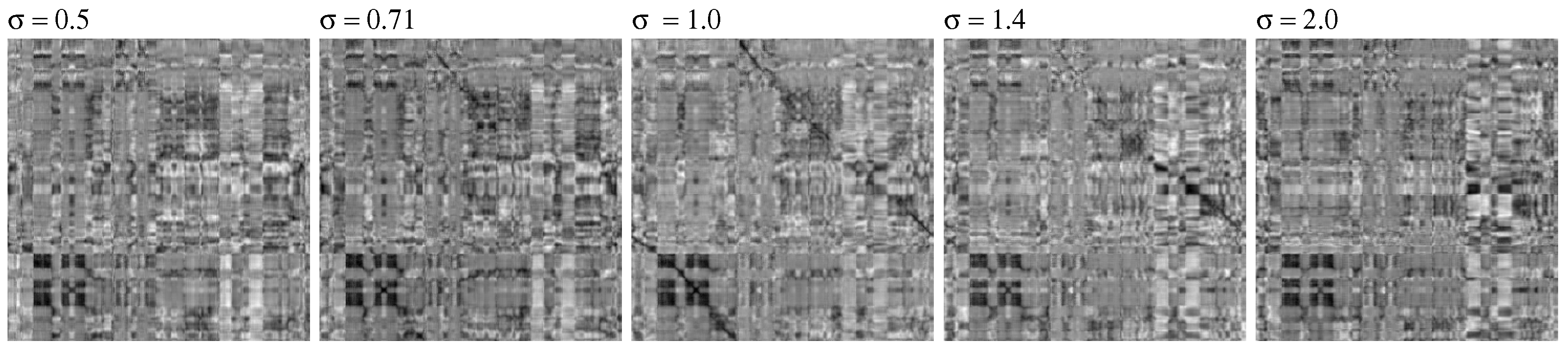
Min-warping does not only compare a single pair of images, but also magnified versions of each image with the original version of the other (see [
20]). Magnification only affects the vertical direction and leaves the horizon unchanged. For efficiency reasons, magnification is performed using nearest-neighbor interpolation between image rows which may lead to duplicated image rows, see
Figure 7. If a first-order vertical edge filter is applied to a magnified column, erroneous zero entries may be produced. We therefore decided to apply the vertical edge filter to the
original two images, and then magnify the
edge-filtered image. However, one has to be aware that exchanging the order of the operations affects the result: If an image (for simplicity in continuous representation) is first magnified (M) and then edge-filtered (ME), the derivatives are effectively multiplied by the magnification factor and therefore scaled down (magnification is achieved for
). Assuming a horizon at
, this can be written as
This has to be considered if the image is first edge-filtered (E) and then magnified (EM), since there the derivatives would remain unchanged:
Here we have to scale the derivatives by multiplying
by
σ to arrive at the same result as in Equation (
7). We will test both versions (with and without scaling of the derivatives).
3.6. Sequential Correlation (SC, TSC)
Sequential correlation and its approximated form (next section) are the major novel contributions of this work. In most of the well-known distance measures like NCC, SSD, PSSD, as well as in the TSSD, TNCC, TZSSD, and TZNCC measures introduced above, the order of the elements in the intensity vectors is of no concern. The fact that the corresponding pixels are adjacent in the image is ignored, and all pixel pairs could as well have been sampled in arbitrary order from the two image columns. For our novel “sequential correlation” measure (SC, or ASC for the approximated version), however, we request that the vectors are ordered such that adjacent elements correspond to adjacent pixels in the image. In natural images, neighboring pixels are known to be strongly correlated, so there is usually a smooth transition of intensities between them, even more so as min-warping prefers slightly low-pass filtered images [
20,
51]. Please note that the “image Euclidean distance” (IMED) [
77,
78] was also motivated by the fact that the traditional Euclidean distance ignores the spatial relationship between pixels (leading to large Euclidean distances for small spatial deformations). Interestingly, IMED is equivalent to computing the Euclidean distance on low-pass filtered images [
77]. The spatial relationship between pixels is ignored by most other distances measures where a two-dimensional
point cloud is analyzed, whereas our measures interpret the sequence
as a sampled two-dimensional
curve. Essentially, it is a vertical edge filter which introduces the neighborhood relationship between pixels in our novel measures, so the same effect could be achieved by applying other distance measures to edge-filtered images (which we test for normalized cross-correlation; see
Section 3.5).
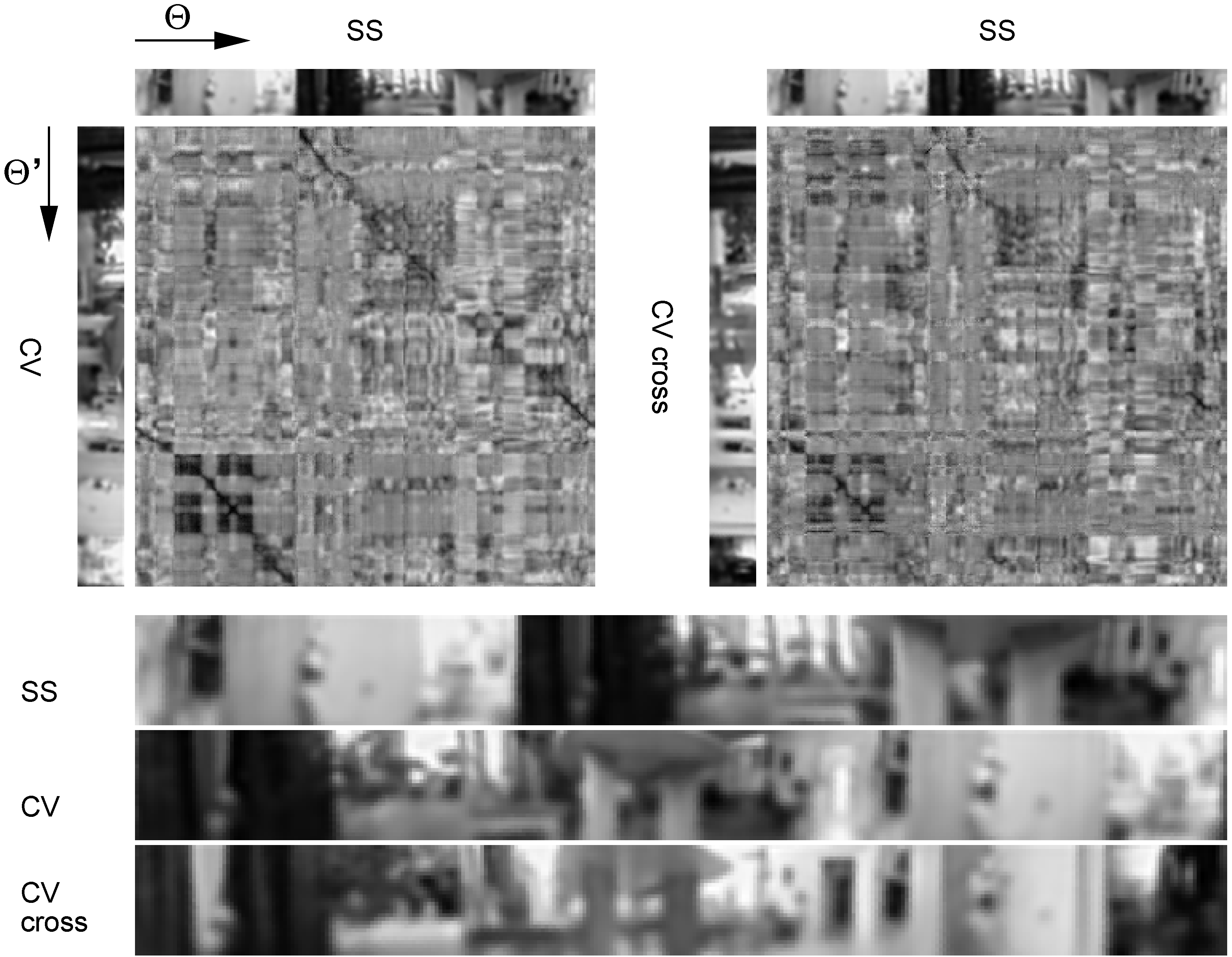
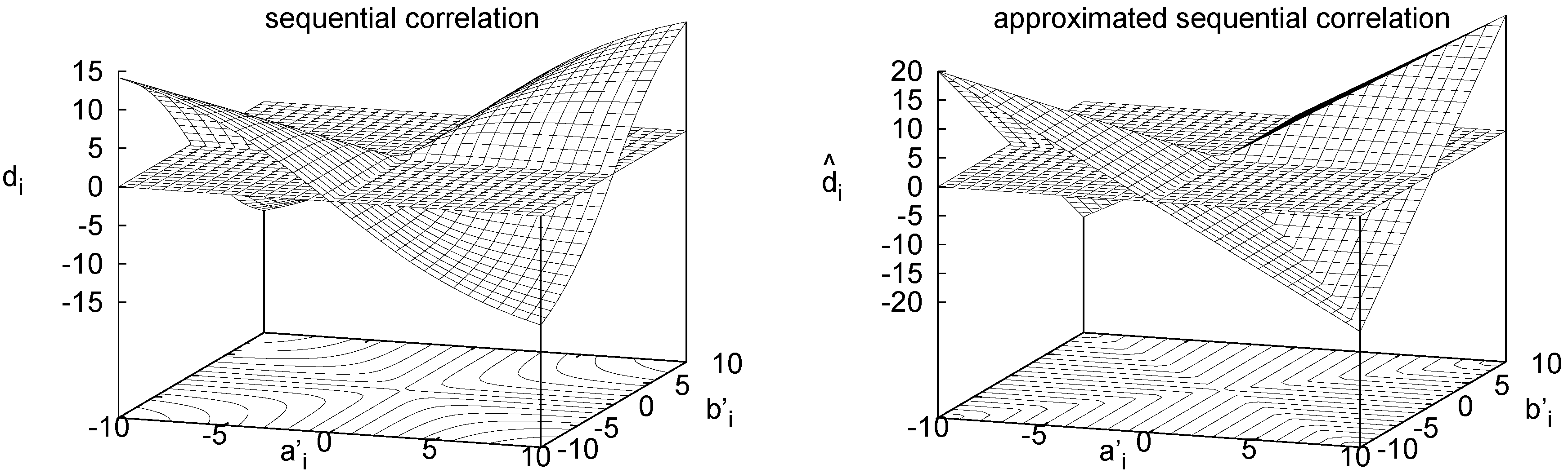
Figure 8 (left) visualizes
.
Figure 8.
Visualization of used in sequential correlation (left) and of used in approximated sequential correlation (right). The zero plane is shown in both plots.
Figure 8.
Visualization of used in sequential correlation (left) and of used in approximated sequential correlation (right). The zero plane is shown in both plots.
For the definition of the sequential correlation measure, we start by defining the segment vector between adjacent sequence points,
This discrete differentiation step introduces shift invariance; see
Section 2. For each segment
i of the sequence, we compute the direction term
where
is the orientation of segment
i with respect to the
axis (see
Figure 9). The second form shows that (for constant
)
will be maximal for
and
(intensity changes in both columns have the same sign and absolute value), and minimal for
and
(intensity changes have the same absolute value but different sign). The first form in Equation (
8) is used in the implementation (since the second contains a slow trigonometric function). Division by
may lead to numerical problems (in our integer implementation, where numerator and denominator are integers, we add 1 to the denominator to avoid this), but the second form shows that at least image noise will not be amplified by this normalization.
We define sequential correlation as
where the second form is used in our implementation. With the standard correlation coefficient (NCC),
shares the range
and the symmetry property. SC is invariant against shifts, here achieved by the transition from intensities to intensity differences, but not invariant against scaling. In the integer-based implementation, we add 1 to the denominator to avoid division by zero in Equation (
10). We test versions with and without scaling of the derivatives; see
Section 3.5. Again, we introduce a tunable form called TSC:
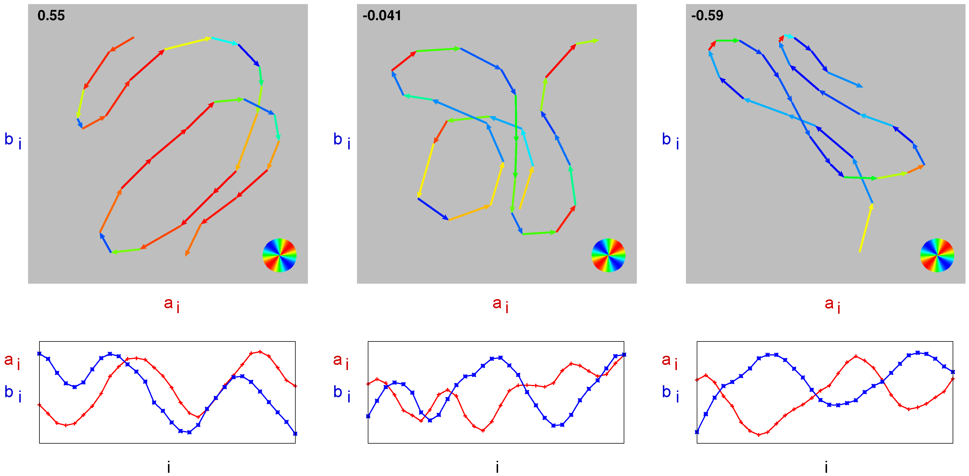
Figure 9.
Visualization of sequential correlation. Top row: intensity sequence . Segment vectors are color-coded according to (see circle on the bottom right). The value of is given in the upper left corner. Bottom row: corresponding individual intensity curves and over i. Left column: positive sequential correlation, center column: approximately zero sequential correlation, right column: negative sequential correlation.
Sequential correlation provides a clear graphical interpretation of correlation on edge-filtered data. In
Figure 9 (top row), the intensity sequence
is shown for three different examples: positive, approximately zero, and negative sequential correlation. The segment vectors are color-coded according to
(red
, blue
). The total length of all segments corresponds to
S, the value obtained by summing the product of segment length
times
gives
D. Their ratio
is specified in the upper left corner.
3.7. Approximated Sequential Correlation (ASC, TASC)
In the implementation of SC, the first form in Equation (
8) is used. This computation is, however, awkward due to the square root required to compute the vector length and due to the division. Our implementation uses 16-bit integer arithmetic with eightfold SIMD (single instruction multiple data) parallelity as offered by Intel’s SSE2 instruction set, but parallel versions of square root and division are not available for this format. Since these operations have to be performed for each segment vector
, the detour via packed floats (4 floats that can be processed in parallel by SSE instructions) results in a marked increase of computation time compared to normalized cross-correlation.
We therefore developed an approximated version of SC, called “approximated sequential correlation” (ASC) which can be implemented almost fully in parallel using just integer instructions. The term
in Equation (
8) was designed such that, for constant
, it becomes maximal at
and
, and minimal at
and
; zero values are achieved for the axis directions (
or
). Moreover, in each direction from the origin, the direction term
is proportional to
. A function with the same properties, but with piecewise linear transition is
see
Figure 8 (right). This approximation of
(up to a constant factor) eliminates square root and division and allows us to implement this computation with eightfold integer parallelity. An equivalent expression is
which saves one operation on CPUs which have instructions for maximum and minimum (as is the case for SSE2 instructions on Intel CPUs); note that the factor 2 can be factored out in Equation (
13) such that it only has to be applied once per column pair. We define
and it can easily be shown by applying the triangle inequality that the measure
lies within the range
. Proof: Triangle inequality:
. Therefore
which ensures
. Define
. Then
which ensures
.
For our implementation, we use
Also ASC is a symmetric measure. As SC, it is only invariant against intensity shifts. An additional advantage is that the two sums of
in Equation (
13) can be precomputed individually for each image column whereas
S in Equation (
9) is inseparable and therefore has to be computed for all column
pairs. To avoid division by zero, we add 1 to the denominator in our integer-based implementation of Equation (
14). We again test versions with and without scaling of the derivatives; see
Section 3.5. The tunable form, TASC, is given by
While ASC is easier to compute,
is not continuously differentiable, and closed-form derivations involving ASC would be hampered by the necessary distinction of cases. In SC,
and
are continuously differentiable except at
, so only this special case has to be handled. So even though SC is computationally more complex, it may still have its value for closed-form derivations, e.g., as a distance measure in gradient or Newton schemes [
40,
41]. It may then be possible to apply a similar approximation as the one between SC and ASC in the final expressions.
3.8. Correlation Measures on Edge-Filtered Images
It may be helpful to present the equations of all correlation measures on edge-filtered images together and in comparable form:
ASC uses an approximation of the numerator of SC, but a different denominator. There cannot be a direct transformation between NCC and SC since NCC is tolerant against scaling and SC is not.
3.9. Correlation of Edge-Filtered 2D Image Patches
In the present form of min-warping, the relations between neighboring columns in the images are not considered since the neighborhood relation changes with the azimuthal distortion of the images and therefore differs between snapshot and current view. Properly including the horizontal interrelations in the search phase would substantially increase the computational effort since optimization techniques like dynamic programming would be required; whether an approximative solution is possible has to be explored. Edge filtering in TENCC/TEZNCC and SC/ASC is therefore only performed in vertical direction within the image columns. For other applications, however, edges can in addition be detected in horizontal direction. Vertical and horizontal differences are simply stacked in a joint vector and compared by the difference measure. An example closely related to min-warping is the visual compass [
25,
44]. Here entire images—in this case sets of all horizontal and vertical differences—are compared by the difference measure for varying relative azimuthal orientation between the two images. Note that, for correlation-type measures, the normalization here only has to be applied once at the end if the distance measure is applied to the entire image rather than to image columns (which of course gives up local illumination invariance achieved by applying the distance measure individually to each image column as done in min-warping).
6. Discussion
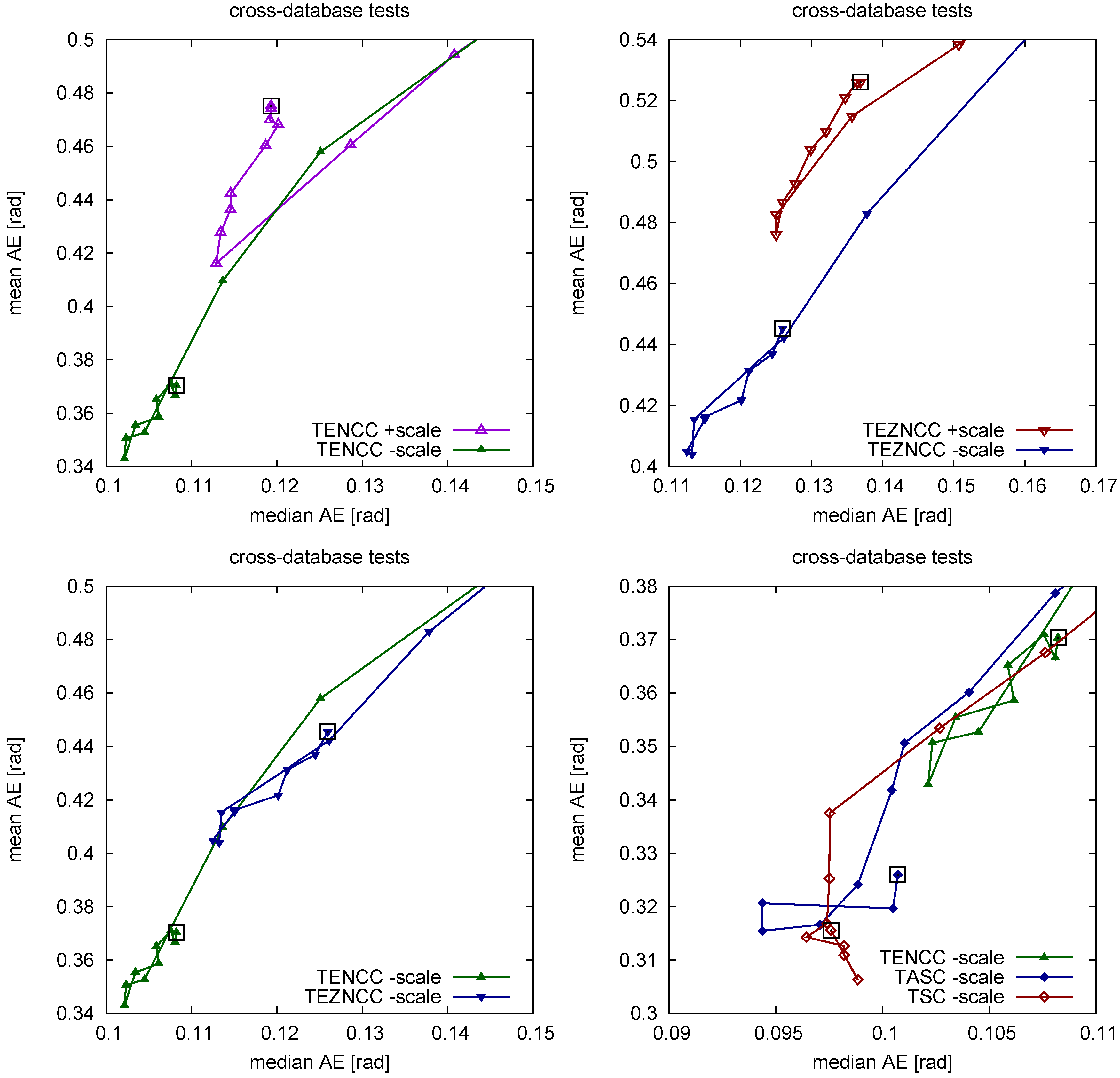
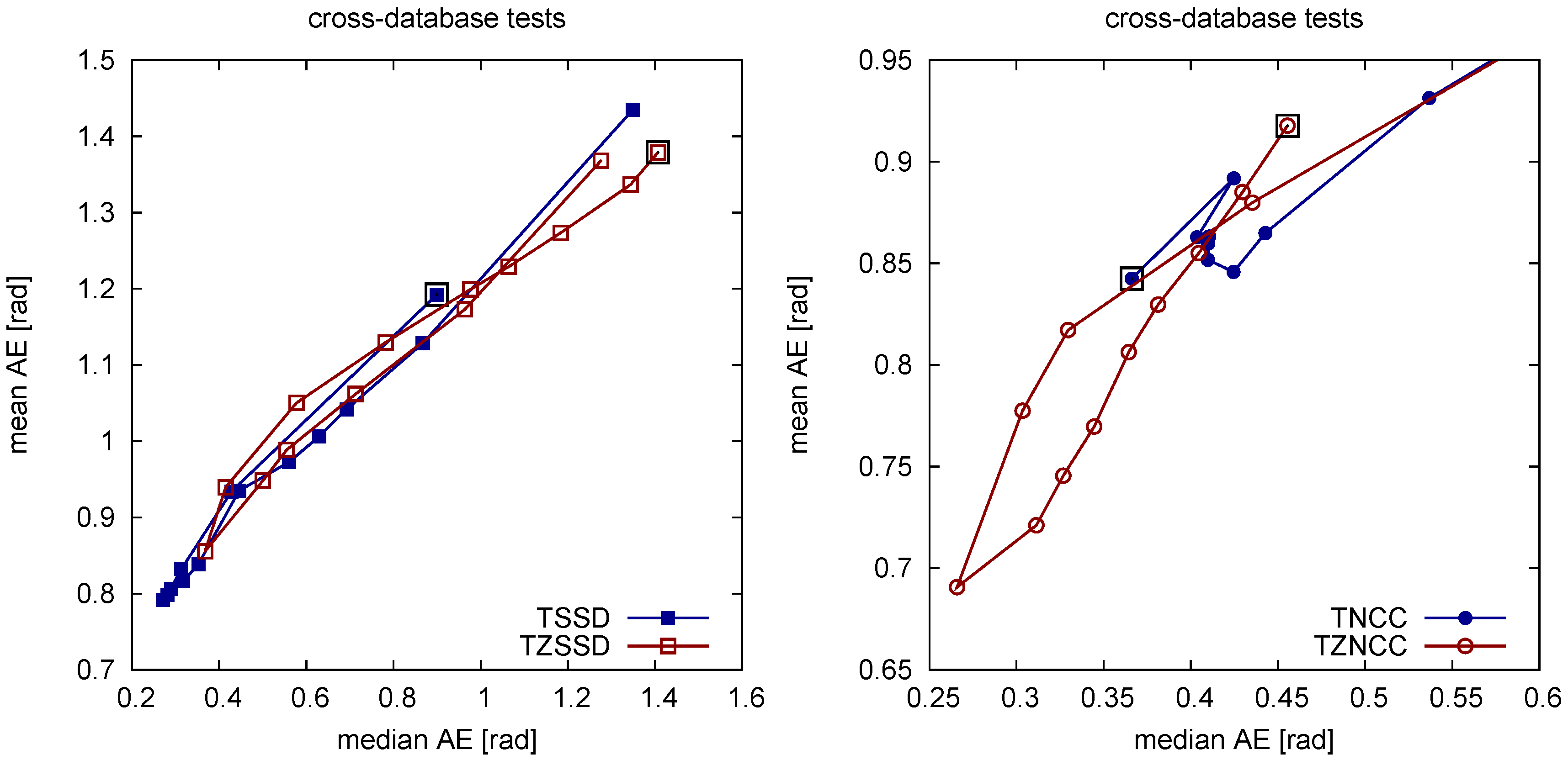
The results show that tunable distance measures which combine an illumination-invariant and an illumination-sensitive term perform best for a certain mixture of the two measures. The illumination-invariant term alone is obviously not sufficient for min-warping which uses all image columns as features without any selection of key points. Whether a tunable distance measure also has an advantage for methods with feature selection has to be explored. For TSSD we can interpret the optimal mixture weight (, obtained for strong illumination changes) since we know that corresponds to the Euclidean distance; compared to the Euclidean distance, the illumination-invariant portion is weighted more strongly. For the other tunable measures we can only say that an intermediate value of w is optimal. TZNCC shows the same behavior (optimum at ), but TNCC seems to be incompatible with the chosen illumination-sensitive term. We didn’t further explore whether another form of illumination-sensitive term would be better suitable since at the measure performs much worse than measures working on edge-filtered images. At least for the illumination-invariant portion alone, we always see that introducing additional tolerance against offsets by subtracting the mean leads to impaired performance compared to tolerance against scaling alone. We assume that double invariance introduces false positive matches.
The better performance of TZNCC over TSSD can be explained by the strong
vs. weak type of scale invariance. Even though we didn’t test other methods with only weak scale invariance such as the co-linearity criterion suggested by [
76] or the image Euclidean distance by [
77], we think that they will also be beaten by measures with strong scale invariance.
Figure 16.
Effect of edge filtering (bottom) on a 1D intensity image (top) where one region became brighter and another region darker (solid to dashed).
Figure 16.
Effect of edge filtering (bottom) on a 1D intensity image (top) where one region became brighter and another region darker (solid to dashed).
Edge filtering (here only tested for the correlation-type measures TENCC and TEZNCC) seems to be the best way to achieve tolerance against illumination changes. While NCC on intensities can only remove intensity scaling affecting the entire image region (in our case an image column), edge filtering works locally within the image region: In sub-regions with constant intensity, differences in intensity are completely removed from the image region, even if one part of the region gets brighter and another one darker (and thus scale invariance with respect to the entire region doesn’t help), and intensity changes only affect the slope of the edges (see
Figure 16). Still, the slope changes can in principle be strong, and we currently can’t present a mathematical analysis that would show why slope changes should be better tolerated by normalized cross-correlation than changes in the intensity image. Whether the fact that neighborhood relations are considered through edge filtering is an advantage is not clear as well. Note that the good illumination tolerance achieved by edge filtering may be paid for by reduced tolerance against spatial translations in the images [
26], e.g., in our example caused by tilt of the robot platform.
If we compare TENCC and TEZNCC, we see that the performance drops if the mean is subtracted, presumably since this step destroys the relation between original and edge-filtered image (very different images can have the same edge-filtered, zero-mean versions, see
Figure 6). The optimal weight of TENCC is
.
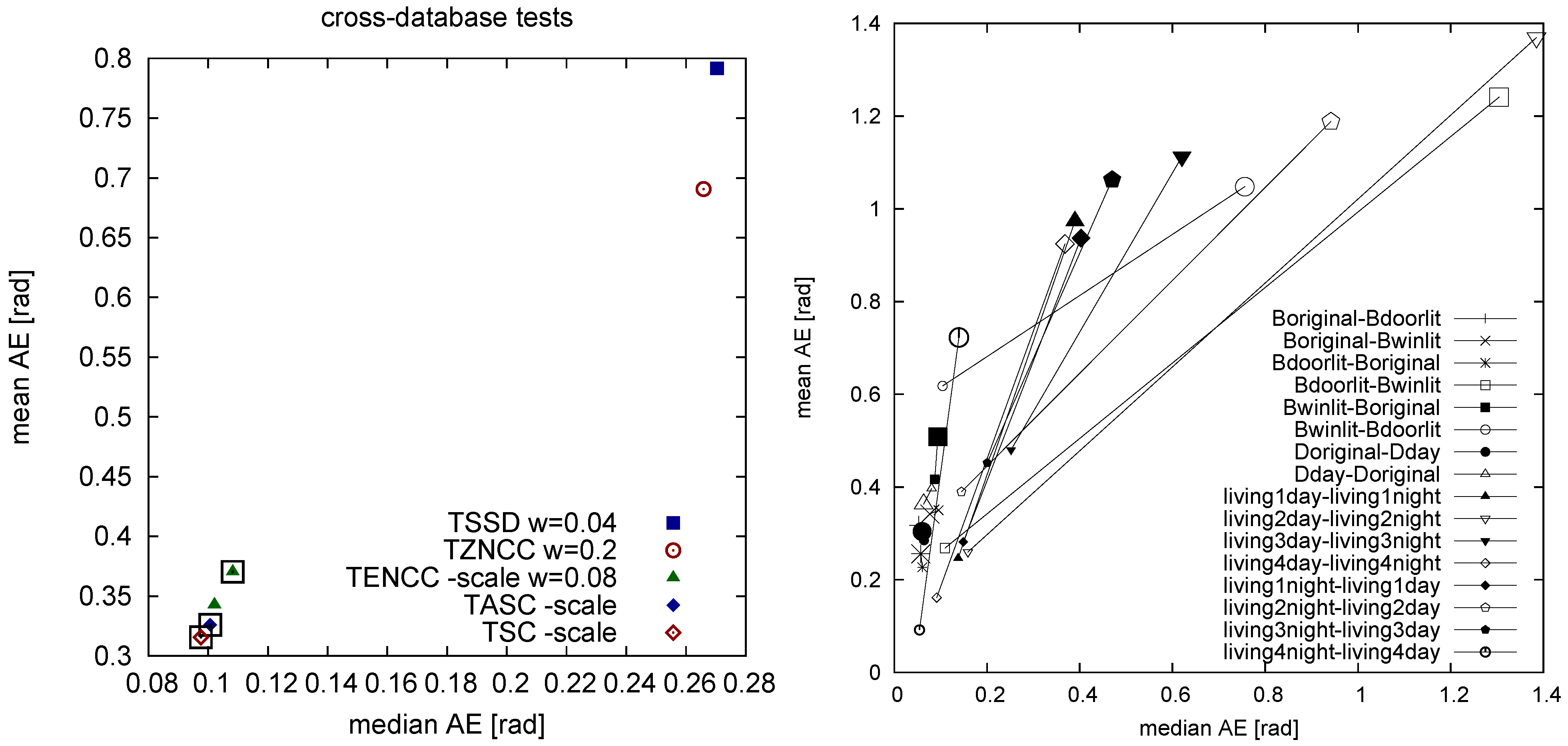
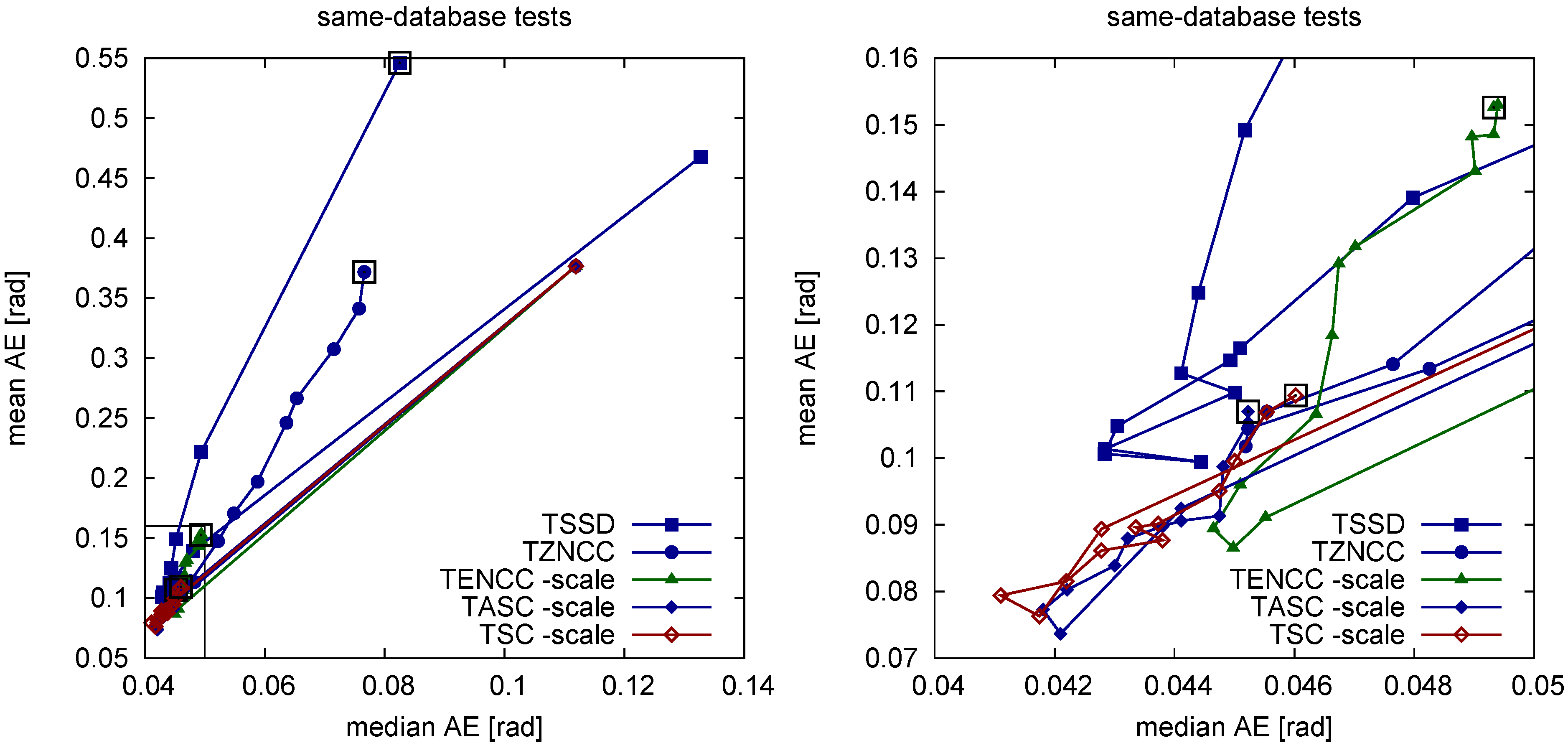
Edge filtering is also the first step of our novel “sequential” correlation measures which treat the two intensity vectors as a sequence of 2D curve points rather than as a mere collection of points without any order. Here the gain achieved by a tunable form is so small that the additional computational effort is not justified. Sequential correlation alone () performs best in cross-database experiments (strong illumination changes) and fairly well in same-database experiments (moderate illumination changes). We could show that the performance gain of sequential correlation compared to the best TSSD method which we obtained for the pooled data is also visible for the majority of the individual databases.
We can only guess why the performance of sequential correlation (SC, ASC) is slightly better than the standard normalized cross-correlation on edge-filtered images (TENCC). Normalized cross-correlation is already (strongly) invariant against scaling, and edge filtering introduces additional invariance against shifts. Double invariance impaired the performance for all distance measures applied to the original images (i.e., without edge filtering), at least for , presumably due to false positive matches introduced by too much tolerance. In contrast, sequential correlation is only tolerant against shifts—as a result of edge filtering—but not against scaling, which may reduce the number of false positive matches.
At the moment we cannot fully explain the following side observation. There are two ways to perform edge filtering in min-warping: Either an image is magnified (in vertical direction around the horizon) first and then edge-filtered, or it is first edge-filtered and then magnified. Since together with nearest-neighbor interpolation we get erroneous derivatives in the first form, we use the second form in our implementation. To achieve the same effect as in the first form, the edge-filtered image should be scaled down if it is magnified. However, leaving out this scaling operation actually improved the performance in all tested methods. We assume that this version of image magnification fits better with the true magnification resulting from decreasing the spatial distance to the feature. Sharp edges may actually have a similar slope regardless of the spatial distance to the feature, but this explanation needs experimental verification.
At least for a fast, integer-based implementation using SIMD instructions (SSE), the original sequential correlation measure requires considerably more computation time than all other distance measures studied here. We suggested an approximated form which can be computed an order of magnitude faster and which does not differ significantly in the navigation performance. We noticed that, compared to normalized cross-correlation, it was easier to chose the float-to-int conversion factors for approximated sequential correlation in accordance with the upper limits imposed by the integer implementation since the method mostly contains additions, subtractions, and the absolute value function but no multiplication.
Invariance against changes in illumination can be established in multiple ways;
Table 3 provides a summary. Weak invariance against
scaling can be achieved by finding the optimal scaling such that the distance (e.g., SSD) between two vectors becomes minimal (parametric SSD measures); strong scale invariance is obtained by normalizing the two vectors to the same length before their distance is computed (NCC measures). Invariance against
shifts can be obtained by either subtracting the mean from the two vectors before they are compared (zero-mean versions of several measures), or by computing the distance between edge-filtered vectors (NCC on edge-filtered images).
Table 3.
Types of invariance of illumination-invariant terms used in the tunable distance measures presented in this work, and navigation performance on databases with strong changes in illumination. Abbreviations: finding the optimal scaling (“scaling”; leads to weak scale invariance), normalizing the vector (“norm”; leads to strong scale invariance), subtracting the mean (“zero-mean”), applying an edge filter (“edge”). The comment “mismatches!” refers to
Figure 6.
Table 3.
Types of invariance of illumination-invariant terms used in the tunable distance measures presented in this work, and navigation performance on databases with strong changes in illumination. Abbreviations: finding the optimal scaling (“scaling”; leads to weak scale invariance), normalizing the vector (“norm”; leads to strong scale invariance), subtracting the mean (“zero-mean”), applying an edge filter (“edge”). The comment “mismatches!” refers to Figure 6.
| Measure | Scale Invariance | Shift Invariance | Navigation Performance |
|---|
| PSSD | scaling (weak) | | |
| PZSSD | scaling (weak) | zero-mean | worse than PSSD (*) |
| NCC+ | norm (strong) | | better than PSSD (*) |
| ZNCC+ | norm (strong) | zero-mean | worse than NCC+ (*) |
| ENCC+ | norm (strong) | edge | much better than NCC+ (*) |
| EZNCC+ | norm (strong) | edge, zero-mean | worse than ENCC+ (*); mismatches! |
| SC+ | | edge | better than ENCC+ (*) |
| ASC+ | | edge | close to SC+ (n.s.) |
We can provide the following explanations for the results:
Normalization is better than scaling of vectors. Normalization (NCC+) turned out to be the better way to achieve scale invariance than finding the optimal scaling (PSSD), even though normalization amplifies noise for short vectors. This can be explained by the fact that NCC+ exhibits strong but PSSD only weak scale invariance.
Invariance against both scaling and shift may lead to mismatches. When only the invariant term of the tunable measure was used, combining invariance against scale and shift always resulted in worse navigation performance than using scale invariance alone. We assume that this is due to increased false positive matches introduced by the double invariance.
Subtracting the mean in edge-filtered images may lead to mismatches. Introducing two-fold invariance against shifts by first applying an edge filter and then additionally subtracting the mean may lead to mismatches as visualized in
Figure 6.
In NCC+, edge filtering is the best way to achieve shift invariance. Even though NCC+ on edge-filtered images is both scale- and shift-invariant, it performs much better than NCC+ on the original intensity images. Edge filtering seems to introduce some kind of local invariance (see
Figure 16) against illumination changes which improves the performance. This is in line with results presented in [
83] where it was derived, by using a probabilistic method, that edge information (specifically the gradient direction) is the best way to accomplish illumination invariance (for object recognition).
Sequential correlation performs best since it only relies on edge filtering. Our novel correlation measures (SC+, ASC+) exclusively rely on shift invariance (and there only on edge filtering); this may explain their small performance advantage over NCC+ on edge-filtered images which is invariant against scale and shift. This stands in contrast to feature-based methods such as SIFT or SURF where apparently tolerance against both shift and scaling is beneficial. As NCC+, also SC+ and ASC+ are correlation-type measures with a normalization which may contribute to their good performance. An additional illumination-sensitive term is not required for SC+ and ASC+.
We did not test
rank-based distance measures such as Spearman’s rank correlation coefficient [
84] which tolerates non-linear illumination changes. Rank-based correlation is not necessarily much more time-consuming since it is applied to each image individually before the two images are interrelated, the latter being the most time-consuming step. However, as we have seen, even simultaneous invariance against both additive and multiplicative changes in intensity resulted in a loss of home vector precision. We therefore expect that the additional tolerance introduced by a rank-based method would further impair the performance.
We also did not test whether a
binary representation of each column vector and a distance computation by the Hamming distance as in the BRIEF, ORB, or FREAK descriptors would improve the performance. This would require an optimization process for the selection of pixels pairs within a column from which the binarized intensity difference are computed [
9]. It is difficult to predict whether such an approach would improve the performance. Binarizing edge-filtered images (
i.e., neighboring pixels form pairs) may impair the performance: Small spatial shifts of the columns introduced by camera tilt would lead to small changes in smooth first derivatives but to larger changes in binarized first derivatives. Binarizing differences between more distant pixels from the column may also not be beneficial: If one part of the column is increased in intensity, local edge filters still recognize the structure in each part whereas differences between more distant pixels may have changed in sign.
All tests described in this paper were performed in two indoor environments, a lab room and a living room, for which cross-illumination databases were available. To the best of our knowledge, there is presently no outdoor image database available where images from the same locations were collected under different conditions of illumination and with sufficiently precise ground truth. We will therefore collect additional cross-illumination databases in indoor and outdoor environments and repeat our tests for these data. For outdoor environments, we have suggested methods where illumination tolerance is achieved by computing contrast measures between UV and visual channels [
85,
86]; it may improve the performance if the distance measures suggested in this paper are applied to data preprocessed by such contrast methods.
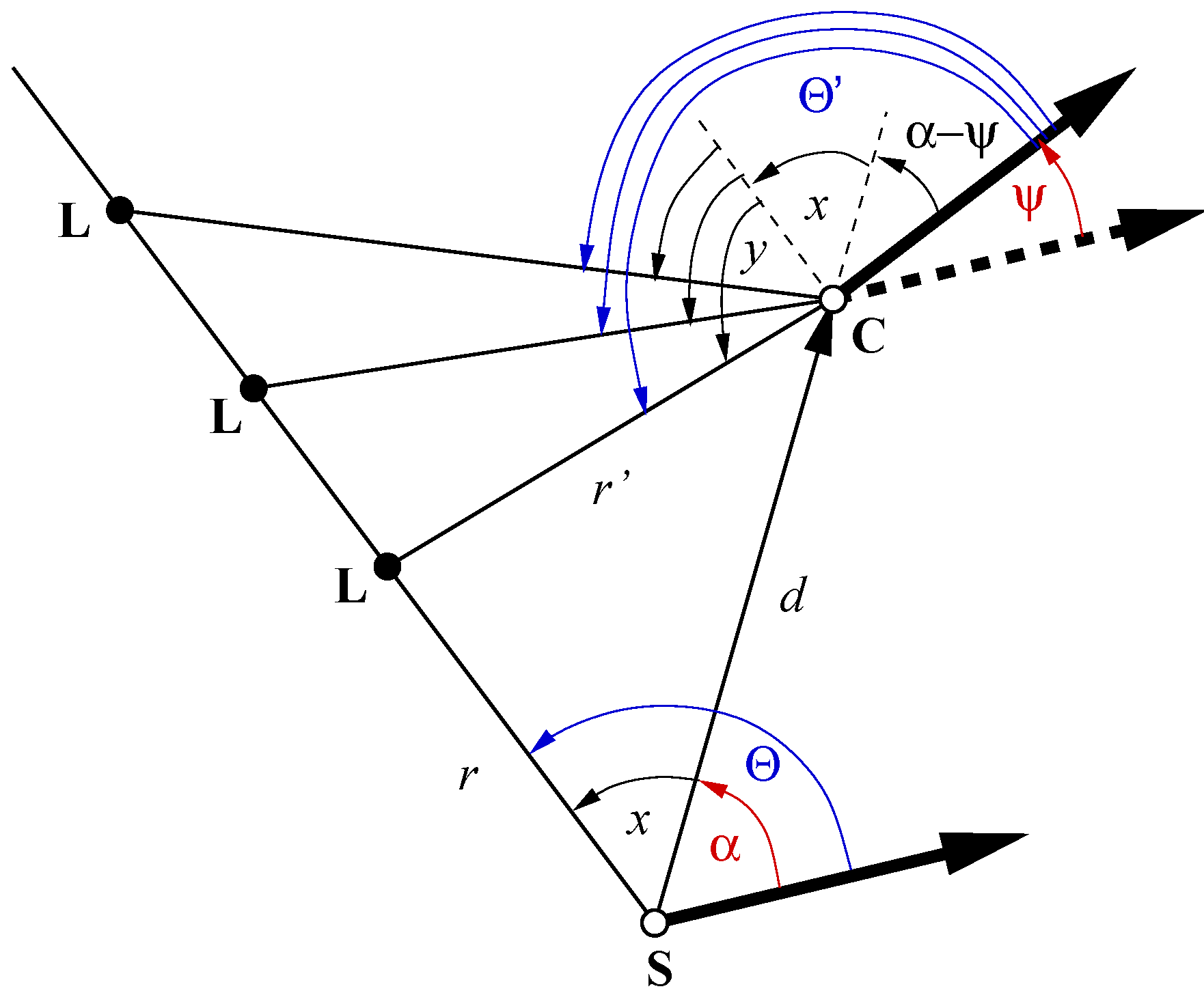
The question whether the results are transferable to other holistic methods, e.g., methods from the DID framework, cannot be answered without systematically investigating these methods. We performed preliminary experiments where we compared the performance of a holistic visual compass method [
25] for the TSSD measure (
) and for the ASC measure. Due to similarities between the first phase of min-warping and the visual compass (see
Section 3.3 in [
20]), we computed a single scale plane using our min-warping implementation and averaged column distances with the same difference angle
; the minimal average provides the rotation estimate. Each randomly rotated snapshot was compared to each randomly rotated current view from the same database or from a cross database, using the same databases as for the min-warping experiments. The mean and median angular error between true and estimated azimuthal rotation were computed.
Surprisingly, here the TSSD measure performed
better than ASC, both for cross-database and for same-database experiments (see
Table 4, first and second row). We can provide the following explanation: Min-warping
distorts and rotates one of the input images according to the simulated movement. For the best match, a large portion of pixels belonging to the same point in space will share the same image position with the other image. In contrast, the visual compass only
rotates one of the images. Therefore the image distortions caused by the spatial distance between the vantage points are not compensated for, and a larger portion of pixels belonging to the same landmark will not appear at the same image position. Since ASC uses edge-filtered images where low image frequencies have been removed, small distances between pixel locations are sufficient to miss a match between edges. TSSD works on intensities and will therefore tolerate larger distortions. This explanation is in accordance with the observation that rotational image difference functions have very sharp minima if low image frequencies are removed [
26]. We expect a similar effect for the DID method where image distortions are not compensated for as well. As a side observation we see from the bottom row in
Table 4 that the rotation estimate obtained from min-warping (which considers image distortions) is much better than the rotation estimate obtained from the visual compass (which doesn’t).
Table 4.
Mean and median angular error [rad] of the compass estimate (ψ) for cross-database and same-database experiments. The first and second row show the results of the visual compass. For comparison, the bottom row presents the error of min-warping’s compass estimate.
Table 4.
Mean and median angular error [rad] of the compass estimate (ψ) for cross-database and same-database experiments. The first and second row show the results of the visual compass. For comparison, the bottom row presents the error of min-warping’s compass estimate.
| | Cross-Database | Same-Database |
|---|
| Method | Mean AE | Median AE | Mean AE | Median AE |
| compass, TSSD () | 0.77 | 0.41 | 0.49 | 0.24 |
| compass, ASC | 0.88 | 0.48 | 0.74 | 0.33 |
| min-warping, ASC | 0.27 | 0.04 | 0.12 | 0.02 |
7. Application: Cleaning Robot Control
In this section, our intention is not to provide a further test of illumination tolerance, but rather to demonstrate that min-warping with the novel approximated sequential correlation measure can successfully be applied to the control of cleaning robots in unmodified indoor environments. With this we hope to dispel doubts that proponents of feature-based methods may harbor on the general applicability of the holistic min-warping method. This is also one of the first robot experiments we performed where we used approximated sequential correlation in the first phase of min-warping instead of TSSD which was used in [
55].
The navigation method used by the cleaning robot is described in detail in [
55]. The robot attempts to cover the entire reachable space by adjoining meander parts. On each meander lane, it collects panoramic snapshot images every 10 cm. It then computes home vectors and compass estimates with respect to snapshot images collected on the previous lane of the same meander part or on a previous meander part. Based on these measurements, a particle filter updates the robot’s position estimate, and a controller corrects the movement direction of the robot such that a lane distance of 30 cm is maintained. Each particle cloud associated with a panoramic view can later be used as landmark position estimate. Views and clouds form nodes of a graph-based, topological-metrical map of the environment which is constructed during the cleaning run.
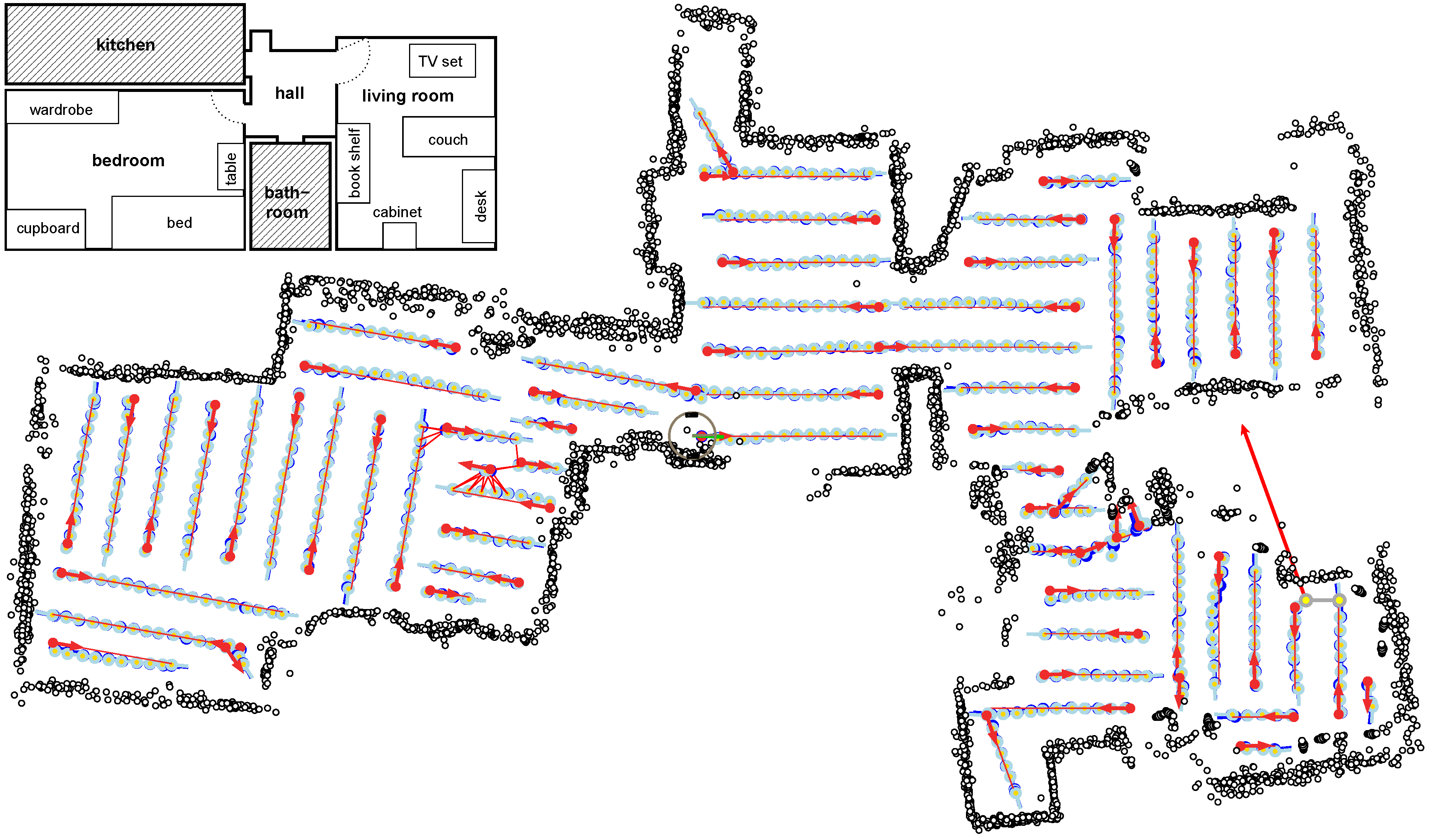
Figure 17.
Internal representation obtained in a cleaning run covering three rooms of an apartment (schematic layout is shown in the inset). Target lanes are shown as red lines. Position estimates (averages of particle clouds) are visualized by light blue circles. Parts of the trajectory where the robot traversed existing meander parts to reach the starting point of a new part are omitted for clarity. Black dots are range sensor measurements. The final position of the robot (close to the starting point of the very first lane) is indicated.
Figure 17 shows the internal representation of the robot’s trajectory for a cleaning run that covers multiple rooms of an apartment. Red lines are target lanes, light blue circles visualize position estimates at all map nodes (averages of particle clouds). It can be seen that a wide portion of the reachable space was covered. (Note that the gap in the range sensor measurements (black dots) close to the robot is actually closed, but the range sensor measurements which originally filled the gap were discarded and could not be replaced by fresh sensor measurements since the robot returned to the start location immediately afterwards and finished the run.) Black dots are range sensor measurements. These are only used to identify uncleaned free space, not for updating the position estimates. Range sensor measurements are attached to the nodes of the topological-metrical map and therefore depend on the position estimates of the corresponding map nodes. When looking at the range sensor measurements it is apparent that even though the map is not fully metrically consistent over several parts, there is not much positional drift within each part—otherwise walls would appear multiple times in the plot. The robot successfully returned to the starting point after finishing the last part (the final position is indicated). Light blue lines depict the snapshot pairings for which min-warping was applied. For each visual correction of the position estimate, typically three home vectors are computed from the current snapshot and three snapshots on the previous lane. The first one, shown in red, points to a snapshot approximately 45 deg from the forward direction, the second one, shown in green, points to the closest snapshot on the previous lane, and the third one, shown in blue, points to the snapshot approximately 45 deg from the backward direction. The quality of the estimates provided by min-warping is apparent from the observation that the home vectors produced by min-warping with ASC almost never switch order (red, green, blue) with respect to their direction and usually correspond well with the estimated direction to the node on the previous lane (light blue). Note, however, that the plots show position estimates, not true positions, and that these position estimates are updated by the same home vectors.
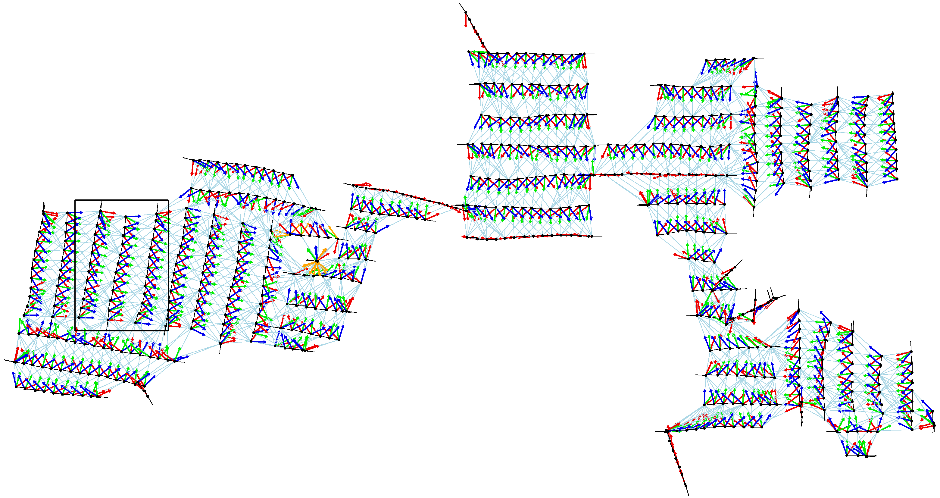
Figure 18 shows all home vectors computed during the cleaning run (compass estimates are omitted for clarity).
Figure 19 magnifies the part indicated by the rectangle in
Figure 18.
Figure 18.
Home vectors (red, green, blue) computed for the update of the position estimate. Light blue lines indicate snapshot pairings from which home vectors (and compass estimates) are computed. The black rectangle indicates the part magnified in
Figure 19.
Figure 18.
Home vectors (red, green, blue) computed for the update of the position estimate. Light blue lines indicate snapshot pairings from which home vectors (and compass estimates) are computed. The black rectangle indicates the part magnified in
Figure 19.
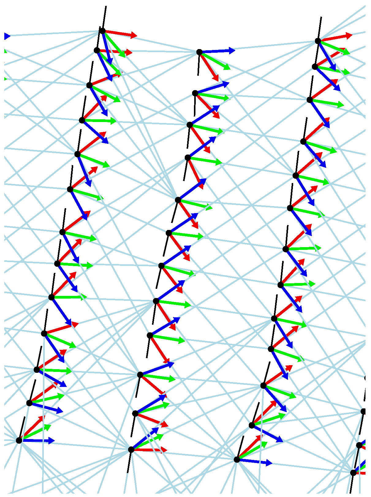
Figure 19.
Magnification of the part enclosed by the black rectangle in
Figure 18. Each robot position estimate is shown as a black dot with a black orientation line.
Figure 19.
Magnification of the part enclosed by the black rectangle in
Figure 18. Each robot position estimate is shown as a black dot with a black orientation line.
A quantitative evaluation of the home vectors is not possible without ground truth (which is not available for this run); our intention is just to give a visual impression. We know, however, that metrical consistency within each meander part is usually good enough to judge homing performance from such a visual inspection [
55].
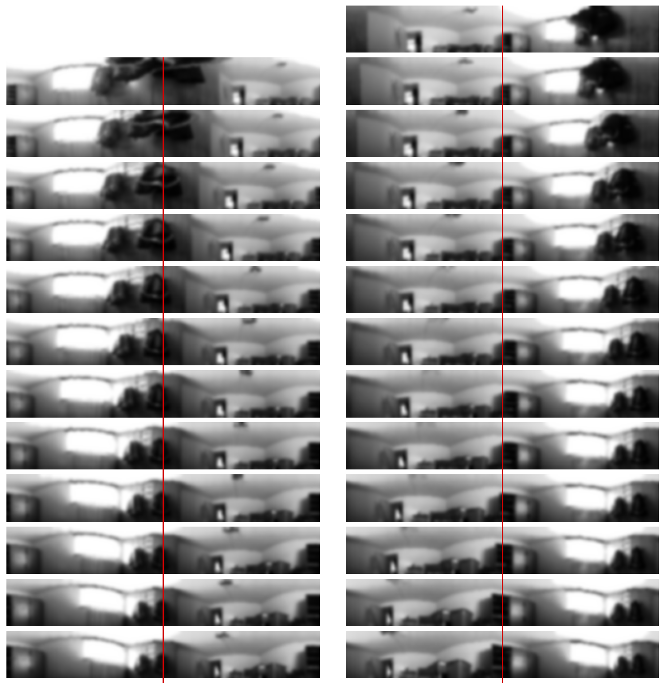
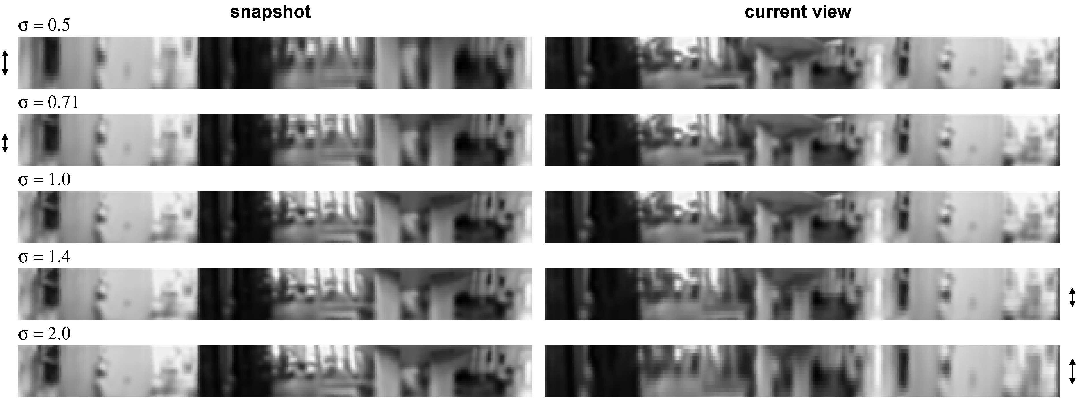
Figure 20.
Images captured on the center lane and the right lane shown in
Figure 19. The images are ordered spatially according to where their corresponding map nodes appear in
Figure 19.
Figure 20.
Images captured on the center lane and the right lane shown in
Figure 19. The images are ordered spatially according to where their corresponding map nodes appear in
Figure 19.
Figure 20 gives a visual impression of the panoramic images (size
) attached to the map nodes of the center lane and the right lane shown in
Figure 19. A red line through the center of each image was added which corresponds to the backward viewing direction of the panoramic camera. Visual features underneath the line shift only by small amounts which indicates that each lane was approximately straight; this corresponds with the position estimates in
Figure 19.


