An Analysis of Power Consumption of Fluid-Driven Robotic Arms Using Isotropy Index: A Proof-of-Concept Simulation-Based Study

Abstract

The manipulability of a robotic arm may be defined based on ease of motion in different directions or ease of applying force/torque. In this study, we use manipulability measures to investigate how the kinematics of robots can be employed to calculate the optimal power required to drive the actuation systems of their arms. We hypothesize that the isotropy measure is related to the power consumption of the robotic arm. In addition to theoretical aspects, we consider practical applications that can minimize power consumption in robotic systems. Since the method is simple to implement and has no assumption on the robot’s work environment or dependence on information on the main power supply, manipulability measures can be used as a tool to predict the power consumption of robotic manipulators.

1. Introduction

Measuring power consumption in robotic systems creates advantages such as increasing the working time of robots without changing the power supplied [1]. Power consumption measures can inform designers of how robotic arms’ weight, size and configuration impact maneuverability and energy efficiency. This is particularly important for robotic systems situated remotely. More efficient energy use has positive environmental impacts, such as decreasing greenhouse gas emissions and slowing the growing demand for energy, especially in emerging economies [2].

To optimize power consumption in robotic systems, it is of the utmost importance to identify quantifiable tools which control and minimize the amount of power required. For instance, if the configuration of a stationary robot is correlated to the power consumed, adding a mobile base to the stationary manipulator would help in altering the configuration. In practice, relocating the base in stationary manipulators is not practical. Redundant stationary robots, however, can be positioned so their posture is optimal for a given task using the path-planning algorithm [3].

In this study, we define quantitative tools related to the energy required to run a system. These tools, the manipulability ellipsoids, help us to visualize how the manipulator configuration of a robot can contribute to its task execution. They visualize the directions and particular properties of arm end effectors [4]. A task is executable if the vectors stay within their ellipsoids.

Manipulability velocity ellipsoids (MVE) and manipulability force ellipsoids (MFE) are very well-known and are valuable tools to analyze, design and control robotic manipulators [5]. The shape of MVE and MFE reflect the constraints to which the robot will be subjected, such as moving or applying force in a specific direction [6]. The ellipsoids do not provide exact numerical information about maximum velocity or force values but suggest directions in which the robot can access or apply force more efficiently [7].

Manipulability measures play significant roles in quantitatively evaluating the efficiency of robotic systems. The manipulability measures indicate the ability to position and orient the end effectors or to apply force or torque. We use Yoshikawa’s measure of manipulability [5], condition number [5], isotropy index [8] and the eccentricity measure of manipulability [9]. In this study, we normalize the manipulability indices for ease of comparison.

The manipulability measures are highly related to the structure and configuration of the robot [10]. For example, when the manipulator is in a singular configuration, the manipulability measures of MVE in some directions become extremely poor, while in others they are very good. Conversely, the robot may be placed in a configuration in which the measures of MVE are identical in all directions. Dexterity analysis is key when designing and evaluating the performance of robotic manipulators. Researchers have used the concept of manipulability to analyze the motion of robotic manipulators for different purposes, often to avoid singular configurations [11,12,13,14].

Although the manipulability ellipsoids are helpful tools in motion analysis of robotic manipulators, they do not offer sufficient information on how fast or slow the manipulators may move along the arbitrary direction or if they suffer from a physical inconsistency when position and orientation information are combined into a single scalar performance parameter [15]. The power manipulability ellipsoid was based on a new parameter that is independent of the selection of mechanisms’ physical unit to overcome the drawback of the physical inconsistency [16]. Specifically, Mansouri et al. [16] presented the concept of a power manipulability ellipsoid: a homogenous tensor defined in six dimensions that includes both translational and rotational components (only motion components of the robotic manipulator). This concept uses a hybrid presentation of the manipulability velocity and force ellipsoids to introduce a vectorial presentation of the power consumed by a robotic manipulator.

The power manipulability ellipsoid had the same drawback as the manipulability ellipsoid and required further modifications to enable us to extract quantitative information on the power and/or kinematic measures. The concept was improved by the authors [17] by forming a quaternion formulation of the power manipulability, previously introduced as a new homogeneous performance index of robot manipulators [14].

In this paper, we utilize the concept of MVE and MFE to define the manipulability power ellipsoid (MPE) to show whether the power consumption and manipulability of a fluid-driven robotic manipulator could be theoretically correlated. We hypothesized that when the isotropy measure of an MPE increases, the robot’s consumed power reduces.

We further conduct a comparative simulation study between the properties of previously used ellipsoids (MVE and MFE) and the newly defined ellipsoid (MPE). The study is conducted using numerical techniques based on assumptions, such as considering quasistatic properties for the hydraulic system. Compared to Mansouri et al. [16,17], our proposed power ellipsoid does not require complex evaluations and mainly focuses on the specification of the fluid-driven actuation system.

2. Materials and Methods

The following subsections explain the concept of manipulability of robotic manipulators and the manipulability ellipsoids and describe the manipulability measures. We then address the power measurements required to drive a fluid-actuated robotic arm. Finally, we define the novel power ellipsoid and describe the test rig and robot equations.

2.1. The Manipulability Velocity and Force Ellipsoids

2.1.1. Jacobian Matrix

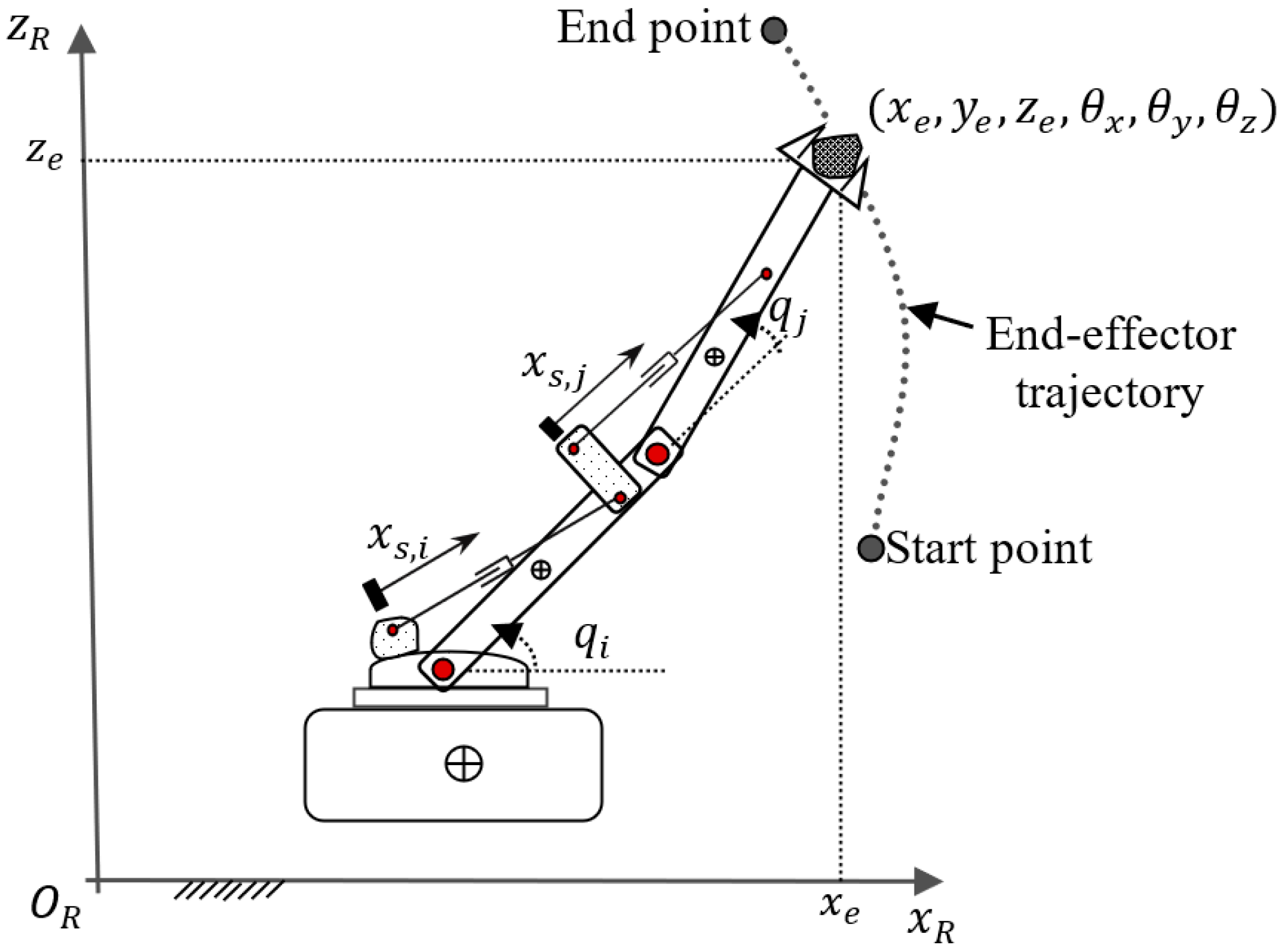
Let ${[x_e{y}_e{z}_e{\theta }_x{\theta }_y{\theta }_z]}^T$ denote the generalized coordinates of the robot’s end effector with respect to the reference frame, $x_R{y}_R{z}_R$, which is composed of parameters describing the robot geometry and joint variables. The reference frame is shown in Figure 1 in the side view ($x_R{z}_R$ plane) of a typical hydraulic manipulator with two degrees of freedom (DOFs): $x_{s,i}$ and $x_{s,j}$. In general modelling, the robot’s end effector possesses six linear and angular velocity components ${[{\dot{x}}_e,{\dot{y}}_e,{\dot{z}}_e,{\dot{\theta }}_x,{\dot{\theta }}_y,{\dot{\theta }}_z]}^T$ with respect to the reference frame {$x_R{y}_R{z}_R$}.

Configuration and velocity/torque limitations are limiting factors affecting the robot’s motion. Increasing the velocities or accelerations of the end effector along the desired trajectory intensifies the effects of the manipulator kinematics and dynamics, which may violate the workability of actuators. Locating the manipulator in an improper configuration can also increase these effects.

An improper configuration is defined when the robot’s configuration is close to the singular situation, e.g., the isometric index is close to zero. Enabling movement along improper trajectories by measuring and improving quantitative tools compensate for the robot’s disability. Since the formulations used in this study are based on the kinematics equations, the following presents the manipulator’s kinematics concept.

The manipulator DOF is denoted by n. Meanwhile, the end effector DOF in Cartesian space is shown by s. Assuming the robot is nonredundant, which means n ≤ s, the Jacobian matrix of the manipulator, $\mathit{J}\left(q\right)$, is given by:

$${\dot{\overrightarrow{X}}}_e=\mathit{J}\left(q\right)\dot{\overrightarrow{q}}$$

(1)

In (1), $\overrightarrow{q }={[q_1\dots q_n]}^T\in {ℛ}^n$, $\dot{\overrightarrow{q}}={[{\dot{q}}_1\dots {\dot{q}}_n]}^T\in {ℛ}^n$ represents the vector of joint angular or linear displacement and velocity for revolute or prismatic joints, respectively. Indeed, $\overrightarrow{q}$ describes the relative displacement between two adjacent links (see $q_j$ in Figure 1).

The end effector velocity vector, ${\dot{\overrightarrow{X}}}_e\in {ℛ}^s$, is generally defined as ${\left[{\dot{x}}_e{\dot{y}}_e{\dot{z}}_e{\dot{\theta }}_x{\dot{\theta }}_y{\dot{\theta }}_z\right]}^T$ when s = 6. Note that if ($\det \mathit{J}\left(q\right)\ne 0$), i.e., when the Jacobian matrix has full rank, the robot would be in a nonsingular condition. In this case, the system can be kinematically evaluated. Hereafter, the dependence on q will be omitted for notational compactness.

2.1.2. Manipulability Ellipsoids

In order to correlate the consumed energy of a fluid-power-driven manipulator to the manipulability concept, we define the existing manipulability ellipsoids: the manipulability velocity ellipsoid (MVE) and manipulability force ellipsoid (MFE). Having these ellipsoids, we can visualize the directions of velocity (MVE) or force (MFE) at the end effector [18]. The definitions of MVE and MFE will later be used to correlate the consumed power to the manipulability of the robot. This helps us observe the variation of the power required to run the robotic manipulator in terms of variations in the robot’s kinematic parameters.

In order to analyze the properties of each manipulability ellipsoid, we use quantifiable tools such as determinants, eigenvalues and eigenvectors. This generalizes the singular value decomposition (SVD) of the mapping matrix (e.g., $\mathit{K}$ and ${\mathit{K}}_{\mathit{L}}$) in the manipulability ellipsoid [19]. Using SVD, some manipulability measures are defined to quantitatively observe the variation of the consumed power.

The manipulability velocity ellipsoid is obtained using kinematics equations and helps us visualize the velocity of the end effector. In (1), if we map the unit circle $\left\{\dot{\overrightarrow{q}}\in {ℛ}^n|||\dot{q}||={\displaystyle \sum }_{i=1}^n{\dot{q}}_i^2=1\right\}$ by $\mathit{J}$ to the space of end effector velocities, ${\dot{\overrightarrow{X}}}_e$, it will result in the manipulability velocity ellipsoid, which is expressed by:

$$\left\{{\overrightarrow{X}}_e\in {ℛ}^s:{\dot{\overrightarrow{X}}}_e=\mathit{J}\dot{\overrightarrow{q}}|||\dot{q}||=1\right\}$$

(2)

This is illustrated in Figure 2. As shown, applying the norm, $||\dot{q}||=1$, results in a circle in the joint space. The circle is mapped through the Jacobian matrix into an ellipsoid in the Cartesian space, called the manipulability velocity ellipsoid. By mapping the normalized value of torque by ${\mathit{J}}^{-T}$, we obtain the MFE.

As concluded from (2) and in Figure 2, in MVE, a Jacobian matrix is shown as the mapping matrix of velocity. Therefore, three submatrices of $\mathit{J}$ are derived as follows:

$$\mathit{J}={\overrightarrow{U}}_{MVE}{\Sigma }_{MVE}{\overrightarrow{V}}_{MVE}^T$$

(3)

where ${\overrightarrow{U}}_{MVE}=\left[\begin{array}{c}{\overrightarrow{u}}_{1,MVE}\dots {\overrightarrow{u}}_{n,MVE}\end{array}\right]\in {ℛ}^{n\times n}$ and ${\overrightarrow{V}}_{MVE}=\left[\begin{array}{c}{\overrightarrow{v}}_{1,MVE}{}^T\dots {\overrightarrow{v}}_{s,MVE}{}^T\end{array}\right]\in {ℛ}^{s\times s}$ are orthogonal matrices and ${\Sigma }_{MVE}\in {ℛ}^{n\times s}$ is a diagonal matrix with non-negative real numbers on the diagonal and can be written as:

$$\Sigma =\left[\begin{array}{ccc}{\sigma }_{1,MVE}& & 0\\ & \ddots & \\ 0& & {\sigma }_{n,MVE}\end{array}|\begin{array}{c}0\\ 0\\ 0\end{array} \right]$$

(4)

where ${\sigma }_{1,MVE}>{\sigma }_{2,MVE}>\dots >{\sigma }_{n,MVE}$ $\left(i=1\dots n\right)$ are the eigenvalues of $\mathit{J}{\mathit{J}}^T$.

The length of each principal axis of the MVE is given by eigenvectors of $\mathit{J}{\mathit{J}}^T$, and the principal axes are shown by ${\sigma }_{n,MVE}{\overrightarrow{u}}_{n,MVE}$. The major axis of the ellipsoid, ${\sigma }_{1,MVE}{\overrightarrow{u}}_{1,MVE}$, corresponds to the direction of the end effector. When the ellipsoid becomes a sphere, the end effector can move with uniform ease in all directions. This type of configuration is called isotropic configuration.

Let $\overrightarrow{{\rm T}}$ be the vector of the joint torque and ${\overrightarrow{F}}_e$ denote the vector of external forces applied to the end effector; then the virtual work theory will result in $\overrightarrow{{\rm T}}={\mathit{J}}^T{\overrightarrow{F}}_e$. Assuming that the manipulator is in a nonsingular condition, the following relationship can be expressed as:

$${\overrightarrow{F}}_e={\mathit{J}}^{-T}\overrightarrow{{\rm T}}$$

(5)

Moreover, the force ellipsoid can be defined by the eigenvalues of ${\left(\mathit{J}{\mathit{J}}^T\right)}^{-1}$, which are equal to $1/{\sigma }_n\left(n=1,2,\dots ,n\right)$. Thus, the principal axes of the force ellipsoid are ${\overrightarrow{u}}_1/{\sigma }_1,\dots ,{\overrightarrow{u}}_n/{\sigma }_n$. While the MVE reflects the uniformity of the velocity of the end effector, the MFE reflects the force/torque applied from/to the end effector.

2.1.3. Manipulability Measures

The manipulability measure is used as a quantitative index to evaluate the performance of the robotic manipulator. For each ellipsoid, we can define measures based on the matrices using SVD. The measures we used in evaluating the dexterity of robotic manipulators are in

Table 1. Manipulability measures used in the simulation study.

Measure	Equation	Description
Yoshikawa’s measure	${\Sigma }_Y=c_n\omega$, $c_n=\{\begin{array}{c}\frac{{\left(2\pi \right)}^{\frac{n}{2}}}{2\times 4\times \dots \times n},niseven\\ \frac{{\left(2\pi \right)}^{\frac{n-1}{2}}}{1\times 3\times \dots \times n},nisodd\end{array}$	Yoshikawa [18]$\mathrm{is}\mathrm{a}\mathrm{measure}\mathrm{of}\mathrm{manipulability}\mathrm{which}\mathrm{is}\mathrm{in}\mathrm{relation}\mathrm{to}\mathrm{the}\mathrm{volume}\mathrm{of}\mathrm{the}\mathrm{ellipsoid}({\Sigma }_Y=c_n\omega$$)\mathrm{where}\omega ={\sigma }_1\dots {\sigma }_n$$\mathrm{and}{c}_n$.
Condition number	${\Sigma }_C={\sigma }_1/{\sigma }_n$ 1	The condition number of a mapping matrix measuring the directional uniformity of the ellipsoid.
Isotropy index	${\Sigma }_I={\sigma }_n/{\sigma }_1$	The ratio of the length of minor semiaxis to the length of major semiaxis of the manipulability velocity ellipsoid.
Eccentricity measure	${\Sigma }_E=\sqrt{1-{\left({\sigma }_n/{\sigma }_1\right)}^2}$	The eccentricity of the ellipsoid and the ability of the end effector to move in a desired direction.

¹ ${\sigma }_1$ and ${\sigma }_n$ are the largest and smallest eigenvalues of $\mathit{J}{\mathit{J}}^T$.

.

2.2. Power Consumption in Fluid-Power-Driven Robotic Arms

In the code developed, the hydraulic system is considered to have quasistatic properties. The actuator dynamics are slowly changing, and the capacitances of the cylinder chambers and hydraulic lines are neglected. Moreover, it is assumed that the mechanical power that enables the actuator to move back and forth is measured at the inlet of the actuator. Since the loss in the values of piping and connections cannot be correlated to the kinematics of the robot, they are ignored.

The 4th order Runge–Kutta method is used to generate the numerical simulation model described in this paper. System parameters used in simulations, formulation of the actuators and the method of modelling are described in detail in Banthia et al. [20].

For the hydraulic actuator shown in Figure 3, the mechanical power supplied by the hydraulic pump is the product of the input pressure and flow of the hydraulic fluid. The equation used to calculate the required power depends on the direction of the link motion when the piston either moves back (${\dot{x}}_s<0$) or forth (${\dot{x}}_s>0$). For the current direction of movement when ${\dot{x}}_s>0$,

$$W_i=P_O{Q}_O$$

(6)

where $P_O$ is the input pressure, supplied by the pump, and $Q_O$ is the flow of the hydraulic fluid. By substituting $Q_O={\dot{x}}_s{A}_O$ into (2), the following equation results:

$$W_i=P_O{\dot{x}}_s{A}_O$$

(7)

where $A_O$ denotes the annulus area of the piston. As shown in (7), the mechanical power required to run the hydraulic link is calculated by measuring the pressure in the inlet chamber, $P_O$ and calculating the linear velocity of the rod, ${\dot{x}}_s$. According to Figure 3, when ${\dot{x}}_{s,i}<0$, the consumed power is obtained using $P_I{\dot{x}}_s{A}_I$.

Bernoulli’s equation is used to express the power in terms of robot kinematics variables. To apply Bernoulli’s equation, it is assumed that the flow is inviscid and steady (velocity pattern constant). The fluid is incompressible, and the friction losses are negligible. In this study, it is also assumed that the energy required for fluid elevation is negligible with respect to the total energy of the system. By applying these assumptions, Bernoulli’s equation for the system shown in Figure 3 is written as in (8).

$$\frac{1}{\rho }{P}_s+\frac{1}{2}{\dot{x}}_s^2=\frac{1}{\rho }{P}_p+\frac{1}{2}{\dot{x}}_p^2$$

(8)

where $\rho$ denotes the hydraulic fluid density. ${\dot{x}}_p^{}$ and ${\dot{x}}_s^{}$ are the linear velocity of the fluid at the outlet of the pump and the inlet chamber of the actuator. The pump output pressure and the inlet chamber pressure are denoted by $P_p$ and $P_s$. Depending on the direction of the link motion, $P_s$ can be either $P_O$ or $P_I$. The pump pressure, $P_p$, is set to be constant.

By applying the continuity equation to the system, given that there is no leakage in the system, the following equation can be written:

$$A_s{\dot{x}}_s^{}=A_p{\dot{x}}_p^{}$$

(9)

Combining (8) and (9) gives the pressure at the inlet chamber:

$$P_s=P_p+K{\dot{x}}_s^2$$

(10)

where

$$K=\frac{\rho \left(A_s^2-A_p^2\right)}{2A_p^2}>0$$

(11)

Substituting (6) into (2) results in:

$$W_i\left({\dot{x}}_s^{}\right)={\dot{x}}_s^{}\left(P_p+K{\dot{x}}_s^2\right)$$

(12)

The angular velocity of the joint, $\dot{q}$, and the linear velocity in the hydraulic actuator, ${\dot{x}}_s$, are related using the geometrical correlation mechanism, shown in Figure 1, as follows:

$${\dot{x}}_s=\frac{d{x}_s}{dq}\dot{q}$$

(13)

For a robot with $n$ DOFs, the total power needed to run all $n$ hydraulic actuators is calculated by summing the power needed for each actuator, i.e., $W={\displaystyle \sum }_{i=1}^n{W}_i$. Equation (13), for the n-DOF robot, can be rewritten as:

$${\dot{\overrightarrow{x}}}_s=D\dot{\overrightarrow{q}}$$

(14)

where ${\dot{\overrightarrow{x}}}_s={[{\dot{x}}_{s,1}\dots {\dot{x}}_{s,n}]}^T\in {ℛ}^n$ is the vector of linear velocity, which is combined with the linear velocity of hydraulic actuators in the manipulator. The vector of the joints angular velocities is denoted by $\dot{\overrightarrow{q}}={[{\dot{q}}_1\dots {\dot{q}}_n]}^T\in {ℛ}^n$. The matrix of velocity, $D\in {ℛ}^{n\times n}$, maps the joints angular velocities to the linear velocity of hydraulic actuators and is given by:

$$D=\left[\begin{array}{ccc}\frac{d{x}_{s,1}}{d{q}_1}& & 0\\ & \ddots & \\ 0& & \frac{d{x}_{s,n}}{d{q}_n}\end{array}\right]$$

(15)

Combining (12) and (14) results in the symbolic form of the power–velocity equation as below:

$$\overrightarrow{W}=K\dot{\overrightarrow{q}}$$

(16)

where $\overrightarrow{W}={[W_1\dots W_n]}^T\in {ℛ}^n$ is the vector of power consumed by each actuator. The mapping matrix of energy, $K$, is defined as follows:

$$K=\left[\begin{array}{ccc}{K}_{11}& & 0\\ & \ddots & \\ 0& & K_{nn}\end{array}\right]$$

(17)

where

$$K_{11}=\frac{d{x}_{s,1}}{d{q}_1}[P_p+\frac{\rho {\dot{q}}_1^2\left(A_{s,1}^2-A_p^2\right)}{2A_p^2}\left(\frac{d{x}_{s,1}}{d{q}_1}{)}^2\right]\mathrm{and}{K}_{nn}=\frac{d{x}_{s,n}}{d{q}_n}[P_p+\frac{\rho {\dot{q}}_n^2\left(A_{s,n}^2-A_p^2\right)}{2A_p^2}(\frac{d{x}_{s,n}}{d{q}_n}{)}^2]$$

(18)

In accordance with the properties of the real hydraulic system, it is observed that $P_p\gg K{\dot{q}}^2{(\frac{d{x}_s}{dq})}^2$. Therefore, the linearized form of the mapping matrix of energy is expressed as:

$$K_L=\left[\begin{array}{ccc}{P}_p\frac{d{x}_{s,1}}{d{q}_1}& & 0\\ & \ddots & \\ 0& & P_p\frac{d{x}_{s,n}}{d{q}_n}\end{array}\right]$$

(19)

The concept presented in (17) and (18) is then used to define the $PE$.

2.3. Power Ellipsoid (PE)

As presented in (17) and (18), the power supplied by the hydraulic pump is directly correlated to the angular velocity of the robot’s joints. In this equation, if we map the unit circle $\left\{\dot{\overrightarrow{q}}\in {ℛ}^n|||\dot{q}||={\displaystyle \sum }_{i=1}^n{\dot{q}}_i^2=1\right\}$by $\mathit{K}$ or ${\mathit{K}}_{\mathit{L}}$ into the space of actuators’ powers, $\overrightarrow{W}$, the MPE is:

$$\begin{gathered} \left\{\overrightarrow{W}\in {ℛ}^n:\overrightarrow{W}\propto \mathit{K}\dot{\overrightarrow{q}}|||\dot{q}||=1\right\}\left(\mathrm{Nonlinear}\mathrm{form}\right) \\ \left\{\overrightarrow{W}\in {ℛ}^n:\overrightarrow{W}\propto {\mathit{K}}_{\mathit{L}}\dot{\overrightarrow{q}}|||\dot{q}||=1\right\}\left(\mathrm{Linear}\mathrm{form}\right) \end{gathered}$$

(20)

Figure 4 depicts the concept of MPE. As seen, the mapping matrix of energy is $\mathit{K}$ in the nonlinear form and ${\mathit{K}}_{\mathit{L}}$ in the linear form.

Here, similar measures for MPE are used to correlate the power consumption and manipulability of the robot. According to the definitions used for the manipulability of robotic manipulators, it can be concluded that by decreasing the isotropy measure of MPE, ${\Sigma }_{I,PE}$, the consumed power by the robot reduces.

Table 2. A qualitative summary of measures defined by MPE and consumed power.

Measure Increased	Power Consumption
$\mathrm{Yoshikawa}’\mathrm{s}\mathrm{measure},{\Sigma }_{Y,PE}$	$\uparrow$
$\mathrm{Condition}\mathrm{number},{\Sigma }_{C,PE}$	$\downarrow$
$\mathrm{Isotropy}\mathrm{index},{\Sigma }_{I,PE}$	$\uparrow$
$\mathrm{Eccentricity}\mathrm{measure},{\Sigma }_{E,PE}$	$\downarrow$

summarizes the qualitative relationship between the manipulability measures of MPE and the power required to run the hydraulic robot. The signs shown in this table indicate the increasing ($\uparrow$) and decreasing ($\downarrow$) relationship between the measures and energy.

2.4. Simulation Setup

The 3-DOF hydraulic robot was modelled and simulated to see whether the ellipsoids had any correlation with the power consumed. Figure 5 depicts the manipulator with coordinate frames assigned to the links. Using the Denavit–Hartenberg notation, the forward kinematics is calculated by multiplying the transformation matrices. The generalized coordinate frames are attached to the robot, which starts from the base frame, {$x_o{y}_o{z}_o$}, and ends at the end effector, {$x_e{y}_e{z}_e$}. The transformation matrix, which correlates the position of the end effector to the base frame, is given by Maddahi et al. [21]:

$$T=\left[\begin{array}{cccc}{c}_{23}{c}_1& -s_1& s_{23}{c}_1& c_1\left(l_1+l_2{c}_2+l_3{c}_{23}\right)\\ c_{23}{s}_1& c_1& s_{23}{s}_1& s_1\left(l_1+l_2{c}_2+l_3{c}_{23}\right)\\ -s_{23}& 0& c_{23}& -l_2{s}_2-l_3{s}_{23}\\ 0& 0& 0& 1\end{array}\right]$$

(21)

In (21), $l_1,l_2$ and $l_3$ are the lengths of robot links, which are shown in Figure 5. $c_i$ and $s_i$ denote $\cos \left({\theta }_i\right)$ and $\sin \left({\theta }_i\right)$, and $c_{ij}$ and $s_{ij}$ represent $\cos \left({\theta }_i+{\theta }_j\right)$ and $\sin \left({\theta }_i+{\theta }_j\right)$, respectively.

To evaluate the manipulability of the robot and to calculate the manipulability measures, the Jacobian matrix is used and is expressed as in (22).

$$J_e=\left[\begin{array}{ccc}-s_1\left(l_1+l_2{c}_2+l_3{c}_{23}\right)& -c_1\left(l_2{s}_2+l_3{s}_{23}\right)& -c_1{l}_3{s}_{23}\\ c_1\left(l_1+l_2{c}_2+l_3{c}_{23}\right)& -s_1\left(l_2{s}_2+l_3{s}_{23}\right)& -s_1{l}_3{s}_{23}\\ 0& -l_2{c}_2-l_3{c}_{23}& -l_3{c}_{23}\end{array}\right]$$

(22)

The specification of the analyzed part of the robot is listed in

Table 3. Link parameters of the simulated 3-DOF robotic arm.

Link	Length (m)	Mass (kg)	Range	Variable
1	0.133	7.3	55°	${\theta }_1$
2	0.549	22.5	90°	${\theta }_2$
3	0.342	15.7	130°	${\theta }_3$

. The dimensions are adopted from CAD drawings. The required parameters for each actuator and the hydraulic system are shown in

Table 4. Hydraulic actuator parameters.

Parameter	Value
Pump pressure, $P_s$	7.2 MPa
Tank Pressure, $P_e$	0 MPa
Piston area (blind side)	3.167 × 10−3 m2
Piston area (rode side)	2.6603 × 10−3 m2
Hydraulic fluid density, $\rho$	847.16 kg/m3
Stoke of cylinder 1, $x_{s,1}$	0.26416 m
Stroke of cylinder 2, $x_{s,2}$	0.15875 m
Stroke of cylinder 3, $x_{s,3}$	0.1016 m

. All actuators have the same parameters with the exclusion of different strokes [22].

The linkage geometry of the manipulator gives the linear velocity of hydraulic actuators (${\dot{x}}_i$) as functions of joint variables (${\dot{q}}_i$) as follows:

$$\begin{gathered} {\dot{x}}_1=\frac{-a_1{a}_2{\dot{q}}_1\sin \left(q_1+{81}^{°}\right)}{\sqrt{a_1{}^2+a_2{}^2+2a_1{a}_2\cos \left({81}^{°}+q_1\right)}} \\ {\dot{x}}_2=\frac{-b_1{b}_2{\dot{q}}_2\sin \left(q_2+{112}^{°}\right)}{\sqrt{b_1{}^2+b_2{}^2+2b_1{b}_2\cos \left({112}^{°}-q_2\right)}} \\ {\dot{x}}_3=\frac{-c_1{c}_2{\dot{q}}_3\sin \left(q_3-2^{°}\right)}{\sqrt{c_1{}^2+c_2{}^2+2c_1{c}_2\cos \left(q_3-2^{°}\right)}} \end{gathered}$$

(23)

where $a_1=253.5\mathrm{mm}$, $a_2=103.4\mathrm{mm}$, $b_1=174.0\mathrm{mm}$, $b_2=538.7\mathrm{mm}$, $c_1=375.9\mathrm{mm}$ and $c_2=165.1$ mm. The constant values in angles are offsets in the joint angles.

3. Results

3.1. Simulation Results

This simulation aimed to measure the power consumed by the hydraulic actuators to run the robot, to calculate the manipulability measures and validate the relationship between the required power and manipulability measures. A program was developed in C++ to emulate the characteristics of this robotic manipulator. The end effector of the robot was programmed to move along a circular path. The actual trajectory of the robot’s end effector is illustrated in Figure 6. The angular displacement of each joint is shown in Figure 7.

Figure 8 depicts the force produced in each actuator and corresponding pressures on both sides of the piston using the mathematical formulation given in Maddahi et al. [22].

By using forces and linear velocities, the power consumed in each actuator is calculated. The angular velocity of each joint is read by the encoders. By using (23), the linear velocity of each actuator is obtained. The variation of pressure is depicted in Figure 9. The total power is the summation of $W_1$, $W_2$, and $W_3$.

Figure 10 depicts the values of manipulability measures for the developed force ellipsoid, MFE, the manipulability velocity ellipsoid, MVE, and the manipulability energy ellipsoid, MPE. The measures include Yoshikawa’s measure (${\Sigma }_{Y,}$), condition number (${\Sigma }_C$), isotropy index (${\Sigma }_I$) and eccentricity measure (${\Sigma }_E$). As illustrated, the relationship between the energy measures and velocity or force measures can, respectively, be found.

The relationship between the total mechanical power required to run the robot and the manipulability measures is illustrated in Figure 11. The experimental results confirm the analytical conclusions, which are presented in Table 1.

By increasing the isotropy index of PE, the required power of the pump increases as shown in the circled area A in Figure 11. Comparing Figure 9 and Figure 10, we find the energy directly changes by altering the Yoshikawa’s measure and isotropy index and has an adverse relationship with the condition number and eccentricity measure. By comparing $\left|\mathit{J}\right|$ and $\left|{\mathit{K}}_{\mathit{L}}\right|$, we conclude that in addition to less energy consumption, which results in minimizing the torque/force of actuators, changing the manipulability can avoid singularity configurations.

3.2. Cross-Correlation Analysis

Cross-correlation analysis was used to investigate the degree to which MPE signals are correlated with the power consumption of the manipulator. Cross-correlation compares data of an MPE signal with a time-shifted (lagged) version of the power signal. To investigate whether a signal is stationary or non-stationary, values of four measures were computed, as shown in

Table 5. Measures used to investigate whether a signal (e.g., values of PE) is stationary or non-stationary.

Measure	Equation	Description
Mean value (first moment)	${\sigma }_{1,PE}=\frac{1}{N}{\displaystyle \sum _{i=1}^N}P{E}_i$	$N$$\mathrm{is}\mathrm{the}\mathrm{number}\mathrm{of}\mathrm{samples}\mathrm{of}\mathrm{the}\mathrm{signal}PE$.
Variance (second moment)	${\sigma }_{2,PE}=\frac{1}{N}{\displaystyle \sum _{i=1}^N}{(P{E}_i-{\sigma }_{1,PE})}^2$
Kurtosis (third moment) 1	${\sigma }_{3,PE}=\frac{1}{N}\frac{{{\displaystyle \sum }}_{i=1}^N{\left(P{E}_i-{\sigma }_{1,PE}\right)}^3}{{\left(\sqrt{{\sigma }_{2,PE}}\right)}^3}$	$\sqrt{{\sigma }_{2,PE}}$$\mathrm{represents}\mathrm{the}\mathrm{standard}\mathrm{deviation}\mathrm{of}PE$.
Skewness (fourth moment) 2	${\sigma }_{4,PE}=\frac{1}{N}\frac{{{\displaystyle \sum }}_{i=1}^N{\left(P{E}_i-{\sigma }_{1,PE}\right)}^4}{{\left(\sqrt{{\sigma }_{2,PE}}\right)}^4}-3$

¹ Kurtosis is the measure of the peakedness of the probability distribution of a real-valued random variable [23]. ² Skewness is the measure of the asymmetry of the probability distribution of a real-valued random variable [24].

.

The cross-correlation coefficient of the MPE signal (PE) and the power consumption signal (PC) for a given window of data is defined as in (24).

$$c{c}_{\tau ,PE,PC}=\frac{1}{N}\frac{{{\displaystyle \sum }}_{i=1}^N\left(P{E}_i-{\sigma }_{1,PE}\right)\left(P{C}_{i+\tau }-{\sigma }_{1,PC}\right)}{\sqrt{{\sigma }_{2, PE}}\sqrt{{\sigma }_{2, PC}}}$$

(24)

In (24), $N$ is the size of the data set or window size of the time series $PE$ and $PC$, and $i$ refers to the $i^{th}$ element from two data sets. ${\sigma }_{1,PE}$ and ${\sigma }_{1,PC}$ are the mean values of $PE$ and $PC$ within the defined window. $\tau$ is an integer value for a time series analysis that determines how far apart the data points which are being compared are from each other (also known as the lag). As observed, the numerator of (24) is equivalent to the covariance of $PE$ and $PC$ with a delay $\tau ,$ while the denominator is the product of the standard deviation of $PE$ and $PC$. In this study, all signals were recorded with $2\mathrm{ms}$ sampling time or at a sampling frequency of 500 Hz.

Both $PE$ and $PC$ signals were examined to investigate whether they were stationary. Results show no upward or downward slope or jump in level in any of the four moments (${\sigma }_1$ to ${\sigma }_4$). The observed trends were steep, exponential or approximately linear; therefore, the signals $PE$ and $PC$ were strongly stationary. It was found that the values of both pairs had a cross-correlation coefficient value of close to 1 (mean of 0.882), indicating that the two signals were similar.

4. Discussion

Manipulability measures and ellipsoids are useful tools to investigate the properties of robot end effectors such as velocity, acceleration and force. They are normally employed as indicators to quantitatively assess the robot’s performance. One of the factors which can be considered to evaluate efficiency is the amount of power required to run the robot. In this study, the manipulability power ellipsoid, $PE$, was defined and correlated to the kinematic parameters of hydraulic manipulators.

To find the relationship between the MPE and consumed power, the coordination systems attached to the manipulator and the Jacobian matrix were first introduced. The manipulability of the robot was defined. We introduced the manipulability velocity, force and energy ellipsoids.

It was demonstrated that the increments of isotropy measure of MPE result in decreasing the consumed power. The concept was validated using a set of simulation studies performed on the main actuators of a 3-DOF robotic manipulator. We propose that the technique to correlate the power measurement to the robot kinematics is practical and provides useful insights for energy consumption. However, more mathematical modelling and validations are required before this correlation can be used as a tool to improve the energy efficiency in applications of hydraulic manipulators.

Quantification of straightforward energy consumption is an important step towards employing energy-efficient robotic systems in a sustainable manufacturing facility. An energy consumption model is normally case-dependent and complex to generate, while requiring continuous updates, as affecting parameters are changing, yet a key to analyze and improve the energy efficiency of robotic systems. Through a proof-of-concept study, we proposed that by implementing the proposed technique in this article, the energy consumption of fluid-driven robotic systems may simply be predicted by understanding and quantifying the characteristics of kinematics measures of the robotic arm, such as manipulability measures.

The proposed algorithm still needs further validations using robotic manipulators with different mechanisms. Therefore, future work will focus on validating the results of the simulation study presented in this paper, using the experimental platform that consists of a set of hydraulic actuators. We are currently conducting a comparative study to investigate the correlation among the MPE, its measures and other existing indices. We are working with machine learning techniques to design an optimal trajectory for a given task while minimizing power consumption.

In the future, this work can be used to find the optimal trajectory for a given task that is based on minimizing the power consumption. This can be done by combining the method and measures provided in this paper with an optimization method, such as genetic algorithms or artificial intelligence, and using the proposed manipulability power ellipsoid (MPE) as the cost function. Studies on the implementation of the same concept for other types of robotic systems, such as electric-driven robotcs, will be conducted in the future, as it is believed that the algorithms could be optimized and polished in order to be used for all types of robotoic manipulators.

References

- Wang, L.; Wang, X. Cloud-Based Cyber-Physical Systems in Manufacturing; Springer International Publishing: New York, NY, USA, 2018; pp. 163–192. [Google Scholar]
- Gabriel, C.A.; Kirkwood, J. Business Models for Model Businesses: Lessons from Renewable Energy Entrepreneur in Developing Countries. Energy Policy 2016, 95, 336–349. [Google Scholar] [CrossRef]
- Papadopoulos, E.; Gonthier, Y. A Frame Force for Large Force Task Planning of Mobile and Redundant Manipulators. J. Robot. Syst. 1999, 16, 151–162. [Google Scholar] [CrossRef]
- Koeppe, R.; Yoshikawa, T. Dynamic Manipulability Analysis of Compliant Motion. In Innovative Robotics for Real-World Applications, Proceedings of the IEEE/RSJ International Conference on Intelligent Robot and Systems, Grenoble, France, 11 September 1997; IEEE: Piscataway, NJ, USA; Volume 3, pp. 1472–1478.
- Yoshikawa, T. Manipulability and Redundancy Control of Robotic Mechanisms. In Proceedings of the IEEE International Conference on Robotics and Automation, St. Louis, MO, USA, 25–28 March 1985; Volume 2, pp. 1004–1009. [Google Scholar]
- Yamamoto, Y.; Yun, X. Unified Analysis on Mobility and Manipulability of Mobile Manipulators. In Proceedings of the IEEE International Conference on Robotics and Automation, Detroit, MI, USA, 10–15 May 1999; Volume 2, pp. 1200–1206. [Google Scholar]
- Melchiorri, C.; Chiaccio, P.; Chiaverini, S.; Sciavicco, L.; Siciliano, B. Comments on “Global task space manipulability ellipsoids for multiple-arm systems and further considerations” [with reply] P. Chiacchio, et al. IEEE Trans. Robot. Autom. 1993, 9, 232–236. [Google Scholar] [CrossRef]
- Balye, B.; Fourquet, J.Y.; Renaud, M. Manipulability of Wheeled Mobile Manipulators: Application to Motion Generation. Int. J. Robot. Res. 2003, 28, 565–581. [Google Scholar] [CrossRef]
- Balye, B.; Fourquet, J.Y.; Renaud, M. Nonholonomic Mobile Manipulators: Kinematics, Velocities and Redundancies. J. Intell. Robot. Syst. 2003, 36, 45–63. [Google Scholar] [CrossRef]
- Merlet, J.P. Jacobian, Manipulability, Condition Number and Accuracy of Parallel Robots. J. Mech. Des. 2006, 28, 199–206. [Google Scholar] [CrossRef]
- Zhou, Y.; Luo, J.; Wang, M. Dynamic Manipulability Analysis of Multi-Arm Space Robot. Robotica 2021, 39, 23–41. [Google Scholar] [CrossRef]
- Wang, Y.; Belzile, B.; Angeles, J.; Li, Q. Kinematic Analysis and Optimum Design of a Novel 2PUR-2RPU Parallel Robot. Mech. Mach. Theory 2019, 139, 407–423. [Google Scholar] [CrossRef]
- Haviland, J.; Corke, P. A Purely-Reactive Manipulability-Maximizing Motion Controller. Available online: https://arxiv.org/abs/2002.11901 (accessed on 23 December 2021).
- Bamdad, M.; Bahri, M. Kinematics and Manipulability Analysis of a Highly Articulated Soft Robotic Manipulator. Robotica 2019, 37, 868–882. [Google Scholar] [CrossRef]
- Choi, H.; Ryu, J. Convex Hull-Based Power Manipulability Analysis of Robot Manipulators. In Proceedings of the IEEE International Conference on Robotics and Automation, Saint Paul, MN, USA, 14–18 May 2012; pp. 2972–2977. [Google Scholar]
- Mansouri, I.; Ouali, M. The Power Manipulability—A New Homogeneous Performance Index of Robot Manipulators. Robot. Comput.-Integr. Manuf. 2011, 27, 434–449. [Google Scholar] [CrossRef]
- Mansouri, I.; Ouali, M. Quaternion Representation of the Power Manipulability. Trans. Can. Soc. Mech. Eng. 2011, 35, 309–336. [Google Scholar] [CrossRef]
- Nguyen, C.C.; Zhou, Z.L.; Mosier, G.E. Analysis and control of a kinematically redundant manipulator. Comput. Electr. Eng. 1991, 17, 147–161. [Google Scholar] [CrossRef]
- Gloub, G.; Van Loan, C. Matrix Computation; John Hopkins University Press: Baltimore, MD, USA, 1996. [Google Scholar]
- Banthia, V.; Maddahi, Y.; Zareinia, K.; Liao, S.; Olson, T.; Fung, W.K.; Balakrishnan, S.; Sepehri, N. A Prototype Telerobotic Platform for Live Transmission Line Maintenance: Review of Design and Development. Trans. Inst. Meas. Control. 2018, 40, 3273–3292. [Google Scholar] [CrossRef] [Green Version]
- Maddahi, Y.; Liao, S.; Fung, W.K.; Hossain, E.; Sepehri, N. Selection of Network Parameters in Wireless Control of Bilateral Teleoperated Manipulators. IEEE Trans. Ind. Inform. 2015, 11, 1445–1456. [Google Scholar] [CrossRef] [Green Version]
- Maddahi, Y.; Gan, L.S.; Zareinia, K.; Lama, S.; Sepehri, N.; Sutherland, G.R. Quantifying Workspace and Forces of Surgical Dissection during Robot-assisted Neurosurgery. Int. J. Med. Robot. Comput. Assist. Surg. 2016, 12, 528–537. [Google Scholar] [CrossRef] [PubMed]
- Abramowitz, M.; Stegun, I. Handbook of Mathematical Functions with Formulas, Graphs and Mathematical Tables; US Government Printing Office: Washington, DC, USA, 1970.
- Brown, R.; Hwang, P. Introduction to Random Signals and Applied Kalman Filtering, 2nd ed.; Wiley: New York, NY, USA, 1992; p. 512. ISBN 0-471-52573-1. [Google Scholar] [CrossRef]
Figure 1.
The coordinate system of a typical 2-DOF hydraulic manipulator.
Figure 2.
Mapping the joint space into Cartesian space using MVE and MFE concepts.
Figure 3.
Schematic of a one DOF robotic arm actuated by the hydraulic system.
Figure 4.
Mapping the angular velocity of joints into the consumed power using the MPE concept.
Figure 5.
Coordinate frames for the 3-DOF robotic manipulator.
Figure 6.
Positional components of the end effector in the simulated task.
Figure 7.
Angular displacement components of the end effector in the simulated task.
Figure 8.
Variations of force in each actuator and corresponding pressures.
Figure 9.
Variation of power in each actuator and corresponding force and linear velocity.
Figure 10.
The MFE, MVE and MPE manipulability measures.
Figure 11.
Total mechanical power required to run the robot and corresponding determinants of mapping matrices of velocity and power.