Model for Origin and Modification of Mass and Coupling Constant


1
Theoretical Physics Division, Chern Institute of Mathematics, Nankai University, Tianjin 300071, China
2
Department of Physics, Tianjin University, Tianjin 300350, China
3
College of Physical Science and Technology, Bohai University, Jinzhou 121013, China
4
College of Physics and Materials Science, Tianjin Normal University, Tianjin 300387, China
*
Author to whom correspondence should be addressed.
Universe 2023, 9(9), 426; https://doi.org/10.3390/universe9090426
Submission received: 8 August 2023
/
Revised: 15 September 2023
/
Accepted: 19 September 2023
/
Published: 21 September 2023
(This article belongs to the Section Foundations of Quantum Mechanics and Quantum Gravity)
Abstract
:We build a model of the origin of physical constants, including masses and coupling constants. We consider the quantum correction of masses and coupling constants. Some exactly solved leading quantum corrections are given. In the model, the physical constant originates from a coupling between the matter field and a background field. We show that if such a background field as it should be in the real physical world is a quantum field, then the physical constant will have a space- and time-dependent quantum correction and will no longer be a constant. We build a scalar field model and a mechanics model. In these two models, we discuss the quantum correction of masses and coupling constants in the field framework and in the mechanics framework.
1. Introduction
We consider the effect of vacuum fluctuations on physical constants. For this purpose, we need a mechanism of the origin of physical constants. There is no generally accepted physical theory about the origin of physical constants. In this paper, we first suggest a model of the origin of physical constants. In the model, the physical constant originates from a coupling between the matter field and a background field. In the model, the physical constant is originated by a mechanism similar to the Higgs mechanism in which the mass of a field comes from a coupling with a scalar field. The physical constants considered in this paper are the mass and the coupling constant.
A real physical field must be a quantum field rather than a classical field. We show that if the background scalar field is a quantum field, there exists a quantum correction on the mass and the coupling constant. The quantum correction is not a constant. As a result, the quantum corrected mass and coupling constant are no longer constants. That is, if the background scalar field is a classical field, the mass and the coupling constant are constants, while if the background field is a quantum field, the mass and the coupling constant may depend on time and spatial coordinates at the quantum level.
In addition to the field-theory model, we build a toy mechanics model. In the mechanics model, the mass and the coupling constant originate from a coupling between the mechanics system and a background mechanics system. Similarly, when the background mechanics system is a quantum mechanics system, the mass and coupling constant have a quantum correction which varies with time and space. This mechanics model helps to explain our point at an elementary level.
The focus of this paper is to explore the possibility of a physical constant being modified at the quantum level. To illustrate the main concept clearly, we construct the toy models as simply as possible, without considering various real physical mechanisms. Along this line of thought, the scheme can be applied to various models and is not limited to masses and coupling constants.
In the model, the matter system is taken as a classical physical system and the background system is taken as a quantum one. However, this model can be directly transformed into the case that both the matter system and the background system are quantum systems, so long as the matter system is a quantum system.
In this paper, we take masses and coupling constants as examples to illustrate how to consider the quantum correction of physical constants. The time-dependent physical constant has been discussed for a long time [1,2]. Jordan considered the variation of fine structure [3,4,5,6]. There are theoretical and experimental studies regarding the gravitational constant. Ref. [7] utilized data from the Wilkinson Microwave Anisotropy Probe (WMAP) to calculate the variation of the gravitational constant G and the parameters in the Brans–Dicke theory and analyze cosmological quantities. Ref. [8] calculated the time-varying gravitational constant G in the context of superstring theory, obtaining a value for and improving the method for measuring . Refs. [9,10] provided upper limits on the variation of the gravitational constant G, , for pulsating white dwarfs and independent constraints on the rate of change. Ref. [11] established boundaries on the evolution of the gravitational constant G in Cosmological Type Ia Supernovae. Ref. [12] proposed a new method to investigate whether the speed of light and fine structure constant vary over time using Strong Gravitational Lensing and Type Ia Supernovae observations, and the result suggested that no strong indication of varying speed of light was found. Ref. [13] provided experimental evidence of the variation of the gravitational constant with space. Ref. [14] demonstrated through experimental data the existence of gravitational dipole radiation, which can be used to test the variation of the gravitational constant. Ref. [15] presented changes in the gravitational constant based on lunar laser ranging data and provided numerical values for and . Ref. [16] considered an -dimensional EGB model and obtained solutions with an exponential dependence of scale factors for the “synchronous-like” variable , which describes an exponential expansion of three-dimensional factor space. The obtained solution satisfied the observational constraints on the temporal variation of the effective gravitational constant G, and the author also provided a detailed analysis of the model’s parameter selection. Refs. [6,17,18,19] discussed basic constants that vary with time in running vacuum models of cosmic evolution. These basic constants include the ratio of the proton mass to the electron mass, the strong coupling constant, the fine structure constant, and gravitational constant. Ref. [20] improved the bounds on the variation of cosmological expansion rates using primordial element abundances, updated nuclear and weak reaction rates, and observations of the cosmic microwave background. The author provided and analyzed and . Ref. [21] improved the Einstein–Hilbert action by using a renormalization group approach and rewrote gravitational constant and the cosmological constant as scalar functions on spacetime. The article also found that a power law indicating a running of Newton’s constant, with a small exponent on the order of , could explain non-Keplerian behavior without requiring the postulation of dark matter in the galactic halo. Ref. [22] considered loop corrections to several physical processes and indicated that the quantum corrections exhibit significant variations, both in magnitude and direction, and do not possess the necessary characteristics of a running coupling constant. In cosmology, there are studies on nonconstant gravitational constant [23]. The method suggested in the paper also applies to the gravitational constant [24]. Some authors discussed the measurement and analysis of the fine structure constant . The quantum correction, generally, may depend on the time and space. Ref. [25] examined the variation of the fine structure constant. The author suggested constructing a variability framework based on general assumptions to discuss the question of whether the fine structure constant changes. In the cosmological context, the framework predicts compatible with astronomical constraints, indicating the possibility of variation in the fine structure constant. However, the author noted that the framework’s prediction of the spatial gradient of conflicts fatally with the results of the Eotvos–Dicke–Braginsky experiments. Therefore, from the perspective of the equivalence principle, the possibility of time variation in the fine structure constant was ruled out. Ref. [26] considered the time-dependent variation of the strong coupling constant. The author proposed to generalize the time-dependent fine structure constant in the Bekenstein model to the strong coupling constant in QCD. It iwas found that the variation of the strong coupling constant in QCD is opposite to that in electromagnetism. Vacuum was identified as the main cause for the variation of the strong coupling constant when compared with the matter. Ref. [27] reviewed progress achieved over the past decade in testing the possibility of time variation of the fine structure constant. The article analyzed the stability of experimental measurements of and the numerical values of . Ref. [28] proposed a new method for measuring changes in the fine structure constant by comparing atomic clocks based on the hyperfine transition in alkali atoms with different atomic numbers. Refs. [29,30,31] also used different atomic clock methods to measure changes in . Ref. [32] demonstrated that quasar spectra can be used to study the possible time or spatial variation of the fine structure constant using a method offering an order of magnitude sensitivity gain. Based on observations from the Keck telescope, Ref. [33] indicated that the value of is smaller at a high redshift, providing evidence for the spatial variation of the fine structure constant. Ref. [34] presented a spectroscopic method for pulsed beams of cold molecules and used this method to measure the frequencies of microwave transitions in CH to search for changes in fundamental physical constants. The article also provided limits on the variations of the fine structure constant and the electron-to-proton mass ratio . There are studies regarding the possible time and space variation of the cosmological constant. Ref. [35] constructed a semiclassical Friedmann–Lemaîre–Robertson–Walker (FLRW) model for the variation of cosmological constants and showed that the cosmological constant becomes variable at arbitrarily low energies due to the remnant quantum effects of the heaviest particles. This model can be validated using Type Ia Supernova observations. It explains that its results coincide with the amplification of obtained from SNAP observations when considering flat FLRW conditions at redshift . Ref. [36] indicated that there is insufficient evidence to show whether or not the cosmological constant is variable or constant and suggested that this problem can only be solved by gaining a deeper understanding of the vacuum contributions of massive quantum fields on a curved spacetime background. The article provided theoretical calculations of cosmological constants or vacuum energies and highlighted that they can vary in QFT. Ref. [37] demonstrated that the presence of quantum gravity leads to an additional contribution to the running charge that does not exist when the cosmological constant is zero.
2. Field-Theory Model: Quantum Correction of Mass and Coupling Constant
In this paper, we build a field-theory model in which the mass and the self-interacting coupling constant originate from a coupling between the matter field and a background scalar field. If the background scalar field is a classical field, the mass and the coupling constant are constants which are the same as that in conventional classical field theory. If the background scalar field, however, as it should be in the real physical world, is a quantum field, the mass and the coupling constant will have a quantum correction. The quantum correction of the physical constant is generally a function of time and spatial coordinate, so the mass and the coupling constant are functions of time and spatial coordinate at the quantum level.
In this paper, we take a scalar field as the matter field as an example.
2.1. Quantum Correction of Mass
2.1.1. Model of Origin of Mass
The free massive matter scalar field is described by the Lagrangian
where m is the mass of the field . In the model, we assume that the mass m originates from a coupling of the matter scalar field to a background scalar field . The background scalar field is described by
where M is a parameter playing the mass of the background scalar field . We couple and in the following form:
The mass term now describes the coupling between and . From the view of the background field , the effective potential is
The mass of the matter field, , depends on the solution of the background field . In the classical field theory, the mass is a constant, so here should be a constant. This requires that the background field is in a time-independent and coordinate-independent classical ground state, i.e., , provided reasonably is lower bounded. In the classical picture, the ground state is the position of the minimum value of the potential . It should be emphasized that in the classical picture it is the position of the minimum value of the potential , rather than the form of the potential , that determines the mass of the matter field ; namely, the mass is . Furthermore, the mass of the field being a constant also requires that the mass is independent of the value of the field . When is zero, i.e., , . At this point, the minimum value point of is also the minimum value point of . Since the mass is a constant, the mass should be determined by the minimum value point of regardless of the value of . Therefore, the minimum value point of must be the same as the minimum value point of . The position of the minimum value of is , which determines that the extremum point of is at . At this point, the function in the term can be chosen arbitrarily as long as the extremum point of occurs at . Therefore, the minimum point of should be at the same position as and .
2.1.2. Quantum Correction of Mass
A field in the real physical world, as it should be, is a quantum field. Here, we consider the case that only the background scalar field is a quantum field.
The mass of the matter field , , depends on the background field , so the quantum correction to the background field leads to a quantum correction to the mass . The quantum correction of is no longer a constant, so the mass is no longer a constant and may depend on the time and the spatial coordinate.
To calculate the quantum correction to the mass , we first calculate the quantum correction to the background field by the path integral approach.
The classical field is given by the classical action functional:
The action . The quantum field is given by
The effective action
is the Legendre transform of the generating functional defined by with
The quantum fluctuation, or the quantum correction of the field, is
Expanding the action around the classical field to the second order and considering the classical field Equation (5) offer
Using the Gaussian integral formula
, we have
Solving J by
gives
Effective action (7) becomes
The equation of the quantum fluctuation , by Equation (6), reads
The above result can also be achieved by directly substituting into the field equation obtained by Equation (5) [38].
The classical field equation of the background field by the Lagrangian (3) reads
where denotes the derivative . The equation of the quantum fluctuation up to the first order, by Equation (15), reads
It can be seen that the quantum correction depends on three factors: the classical solution of the background field , the function form of , and the solution of the matter field . The quantum correction is different when the solution of the matter field is different. In the classical picture, the mass of the matter field is independent of the matter field but depends only on the ground state of the background field, while the classical ground state is a constant depending only on the position of the minimum value of .
The quantum correction to the mass of the matter field is determined by the quantum fluctuation . We expand the mass of the matter field around as
where for is the minimum value. The quantum fluctuation can only be determined up to a constant factor, for and are both the solutions of linear homogeneous Equation (17). One can measure the experimental value of the mass at the point . At the point , the quantum corrected mass by Equation (18) up to the leading order is
Then, we have
The undetermined constant can be solved from Equation (21).
The quantum correction is different for different , so we first solve from the field equation given by the Lagrangian (3),
Taking only the leading contribution into account, we simply take . Equation (22) then becomes
Field Equation (23) has the solution
As an example, we consider the case that the matter field is in the ground state. In the ground state, and , so Equation (17) reads
The quantum fluctuation, after separating variables , is given by equations
where is the variable separation constant.
The quantum correction, by solving Equations (26) and (27), are
where is the odd Mathieu function and is the even Mathieu function [39].
The quantum fluctuation should vanish when the mass is very large, i.e., , so we only need the odd Mathieu function:
The quantum corrected mass, when the matter field is in the ground state, by Equation (18), reads
The quantum correction to the mass depends both on the time t and the spatial coordinate x. Once the quantum fluctuation is in the ground state, i.e., , the quantum correction depends only on t:
The quantum corrected part is not a constant which, of course, is small compared to the classical mass.
For the case of , the constant C becomes
2.2. Quantum Correction of Coupling Constant
2.2.1. Model of Origin of Coupling Constant
The same scheme applies also to the quantum correction of the coupling constant.
The matter scalar field with a self-interaction is described by
where we extract the coupling constant out of the potential.
As above, we assume that the coupling constant originates from a coupling of the matter scalar field to a background scalar field . The background field , described by the Lagrangian (2), couples with the matter field in the following form:
The coupling constant serves as a potential of the background field . For the background , there exists a potential
The classical solution of should be a constant solution so that is a constant, for the classical coupling constant is a constant, so . The classical ground-state solution is the position of the minimum value of . The classical coupling constant is independent of , which requires that the coupling constant depends on and only on the background field . Meanwhile, we also require that the coupling constant should not depend on . When , we have . At , the minimum point of is also the minimum point of . Since the coupling constant is a constant in the classical case, it should be determined by the minimum point of regardless of the value of . Therefore, we require that and have the same minimum point. The minimum point for is , which leads to the minimum point of also being . At this point, the coupling constant in the first term can be arbitrarily chosen without affecting the conclusion that the minimum point of is at . Therefore, the minimum points of should be the same as those of and .
2.2.2. Quantum Correction of Coupling Constant
When the background scalar field is a quantum field, there is a time- and/or space-dependent quantum correction to the coupling constant.
The classical field equation of the background field, by Equation (36), reads
The equation of the quantum fluctuation up to the first order, by Equation (15), reads
Similar to Section 2.1.2, the quantum correction up to the leading contribution is
In the experiments, one can measure the value of the coupling constant at the point . At the point , by Equation (40), up to the leading order, we have
Then, . The quantum fluctuation at , then, by Equation (41), reads
The undetermined constant in can be solved from Equation (42).
The equation of the matter field by the Lagrangian (36) reads
To sketch the model, we consider a simple toy example with the potential
with . Taking only the first-order contribution into account, we take . Then, Equation (43) becomes
which has the solution . As a simple example, we only consider a single mode solution of :
By separating variables , we arrive at
The quantum fluctuation should vanish when the mass tends to infinity, so . Then,
where . The quantum corrected coupling constant is
Once the quantum fluctuation is in the ground state, , the quantum correction depends only on the time t:
Here, is the classical coupling constant.
3. Mechanics Model: Quantum Correction of Mass and Coupling Constant
To illustrate the model intuitively at an elementary level, moreover, we build a mechanics model. In the model, the physical constant, e.g., the mass and the coupling constant, originates from a coupling between the matter and a background background matter. As in the above, in the classical picture, the mass and the coupling constant of a mechanics system are constants. However, in the quantum picture, since the background matter obeys quantum mechanics, the mass and the coupling constant have a quantum correction which varies with time and/or space.
3.1. Quantum Correction of Mass
In classical mechanics, a system is described by the Lagrangian
In the model, we assume that the mass originates from a coupling between the matter mechanics system and a background mechanics system. We introduce a background mechanics system
Here and after, we call the matter system the x-system and the background system the y-system for convenience.
We couple the x-system and the y-system in the form
where is the mass of the x-system and a potential of the y-system. The kinetic energy term describes the coupling between x- and y-systems.
The potential of the y-system is
As discussed above, the y-system should stay in a time-independent stable state. A reasonable choice is , a classical motionless state. In classical mechanics, the motionless solution is the position of the minimum value of . The mass of the classical x-system should be independent of the solution, so we require that the mass should be independent of x. When , , so the minimum point of is the same as the minimum point of . Since the classical mass is a constant, it should be determined by the minimum point of , regardless of the value of x. Thus, and should have the same minimum points. At this point, the mass in can be arbitrarily chosen as long as it does not affect the minimum point of , so the minimum point of should be the same as the minimum points of and , i.e., .
In this model, the mass in the x-system is determined by the position of the minimum value of the potential in the y-system:
with determined by
If the background y-system obeys classical mechanics, the mass depends only on the position of the minimum value of the potential in the y-system, no matter what the function form of the potential is. If the background y-system obeys quantum mechanics, there is a quantum correction to the mass. The quantum correction is no longer a constant.
In classical mechanics, the background y-system is in the classical ground state so that the mass is a constant. In quantum mechanics, the y-system is still in the ground state, but the energy level is discrete. There exists an energy gap which ensures an nonzero mass. The quantum corrected mass is no longer a constant, but may depend on time and space.
Following the method in quantum field theory used above, we write the quantum-corrected solution of the y-system as
where is the is the classical ground state. The mass can be expanded as
where for is the minimum value of .
Here, we use an alternative approach to derive the equation of . Substituting Equation (61) into Equation (57) and keeping only the first order in , we arrive at
Taking Equation (57) into consideration, we arrive at
and are both the solutions of Equation (64). One can measure the experimental value of the coupling constant at the point . At the time , the experimental value is and the quantum corrected mass by Equation (40) up to the leading order is
Then, we have . The quantum fluctuation at , then, by Equation (41), reads
The undetermined constant in can then be solved.
The solution of the classical y-system, , is the ground-state solution: with the position of the minimum value of the potential of the y-system.
The quantum fluctuations for different states of the x-system are different, for , from Equation (64), depends also on the solution of the x-system.
As the leading contribution, we only consider the classical solution of x-system. For the classical x-system, we have , whichs gives
To illustrate, we consider a simple toy model with the potential . In principle, the x-system is also quantum, but as the zero-order approximation we consider the classical equation of motion instead:
where is the classical mass. Equation (69) has a solution , so
The solution is
The quantum effect should vanish when the mass M tends to infinity. When , . The term does not vanish, so . We have
The quantum corrected mass by Equation (62) reads
By observation, the coupling constant measured at is , and determines the constant C:
The quantum correction to the mass depends on the solutions of both the x-system and the y-system.
3.2. Quantum Correction of Coupling Constant
Suppose the matter x-system, , couples with the background y-system as
Here, is the coupling constant in the x-system, but is a potential in the y-system. The classical mechanics equations of motion, by the Lagrangian (76), read
In the y-system, the potential is
Based on the same reasons above, in can be arbitrarily chosen as long as it does not affect the minimum points of , so the minimum points of should be the same as those of and , i.e.,.
The coupling constant in the x-system is determined by the position of the minimum value of the potential of the y-system: with determined by Equation (60). Expanding the coupling constant, we have
where .
The equation of the quantum fluctuation is obtained by substituting Equation (61) into Equation (78) and keeping only the first-order contribution:
Here, and are both solutions.
At the time , the experimental measured value is and the quantum corrected coupling constant by Equation (80) up to the leading order is
Then, we have
The quantum fluctuation at , then, by Equation (82), reads
The undetermined constant in can be solved from Equation (84).
Also, we take the potential as an example. Using the classical equation of motion
as the zero-order approximation, we have a solution of the x-system:
where . In this toy model, we take . Then, the equation of the quantum fluctuation (81) becomes
Similarly, in consideration of that the quantum fluctuation should vanish when M is large, the solution of Equation (87) is
Then, the quantum corrected coupling constant by Equation (80) reads
By observation, the coupling constant measured at is . Then, , by Equation (31), determines the constant C:
4. Discussions and Outlook
We build a field model and a mechanics model of the origin of physical constants. In the field model, the mass and the coupling constant originate from a coupling between the matter field and a background scalar field, so that there is a time- and space-dependent quantum correction. In the mechanics model, the mass and the coupling constant originate from a coupling of the mechanics system with a background mechanics system. If this background mechanics system is a quantum mechanics system, there is a time- and space-dependent quantum correction on the mass and the coupling constant.
By background fields or mechanical systems we mean that we leave aside the observation of this field or mechanical system for the time being, just like the situation that the Higgs field before the Higgs particle was discovered. If the model is correct, the background field, like the Higgs field, should also be observable, but we do not discuss that in this paper.
In this paper, we only consider simple conceptual toy models. In more realistic and therefore more complex cases, the choice of the background scalar field takes into account more factors. But from such a simple model, we can already see that if the physical constant originates from a coupling between the matter and a background matter, then the physical constant is not a constant but varies in time and space. Therefore, whether the physical constant varies in time and space can serve as an experimental criterion to judge whether the model is correct.
It is worth noting that if the physical constant originates from the coupling with a background quantum system and the background field is in a bound state, the physical constant, e.g., the mass and the coupling constant, likely has a nonzero minimum. This implies that in the model, even if the physical constant in the classical picture tends to zero, there will exist a nonzero quantum correction. In other words, the physical constant will have a minimum value, similar to the energy gap.
In the model, the matter fields are classical fields, though the background fields are quantum fields. This is because treating the background field as a quantum field and the matter field as a classical field can already offer the leading order contribution of the quantum correction to physical constants. The same processing applies also to the case where the matter field is a quantum field. Another question that warrants discussion is the effect on physical constants when a transition occurs between two vacuums.
In our model, both the mass and the coupling constant originate from a coupling between the matter field and a background field. If the background field that originates the mass and the coupling constant is the same field, that is, the matter field obtains both of its mass and coupling constant in the same interaction with the background field, then there is some relationship between the mass and the coupling constant. This can be used as a candidate model for the problem of the mixing of the mass eigenstates and the interaction eigenstates of different generations of particles in particle physics. Concretely, in the present paper, to more clearly illustrate the mechanism of generating physical constants proposed in this model, we chose an extremely simple scheme as an example: the matter field is a scalar field, the mass and coupling constants are generated independently, and the effective potential has only one minimum point. This model also applies to the mass and coupling constants for spinor and vector fields. In further work, we will consider more complex and realistic situations: the matter field is a spinor field, and mass and coupling constants are generated through interactions with the same background field. In particular, the effective potential has three distinct minima of different magnitudes, corresponding to three different minimum points. The three different minimum points of the effective potential correspond to three different masses. After considering quantum corrections, these three masses, i.e., the three minima of the effective potential, can transition between each other, while there exists a certain relationship with the coupling between matter fields. This provides a model for three generations of fermions, in which there is a certain relationship between the mass eigenstates and the interaction eigenstates, manifesting as some mixing between the mass and interaction eigenstates. Furthermore, the masses and coupling constants of the different fields in theory, which are independent phenomenological parameters in the current theory, have a common origin, providing a pathway to discussing the relationships between these physical constants and reducing the number of independent phenomenological parameters. In addition, the method presented in this paper is not only limited to obtaining mass and coupling constants, but can, in principle, also be used to consider the origin of other physical constants. If all physical constants arise from the interaction between matter fields and one or several background fields, then the relationship between different physical constants can be described.
In our model, masses originate from the interaction between a matter field and a certain background field. In Mach’s principle, the mass is determined by all other matter in the universe; that is, the mass is not an inherent property of the matter itself but is instead a consequence of the collective interactions of matter in the universe. This similarity inspires us to consider using our model to construct physical models that respect Mach’s principle.
The variation of the physical constant with time and space is a pure quantum effect. In future work, we will discuss the effect of such quantum corrections on various properties of matter fields, e.g., the one-loop effective action, the vacuum energy, and other spectral functions [40,41,42,43,44,45,46]. We may calculate the one-loop effective action, the vacuum energy, and other spectral functions of the quantum field under the quantum-corrected physical constant.
In order to illustrate our treatment at an elementary level, we build a mechanics model to demonstrate the origin of physical constants. In this mechanics model, we suggest a method to approach the quantum result from a classical mechanics model. This method can be further developed on broader issues.
This paper considers toy models in which the matter field is a scalar field rather than the matter fields measured in experiments, such as spinor and electromagnetic fields. Therefore, it cannot be directly compared with current experimental results. However, the approach of modifying the model for physical constants can also be applied to other physical constants associated with other matter fields. In future work, we will consider the modification of physical constants related to matter fields, such as spinor and vector fields. The results obtained can then be compared with experimental results, in principle.
Author Contributions
All authors contributed equally to this work. All authors have read and agreed to the published version of the manuscript.
Funding
This work is supported in part by Special Funds for theoretical physics Research Program of the NSFC under Grant No. 11947124, and NSFC under Grant Nos. 12075167, 11575125, and 11675119.
Data Availability Statement
Not applicable.
Acknowledgments
We are very indebted to G. Zeitrauman for his encouragement.
Conflicts of Interest
The authors declare no conflict of interest.
References
- Dirac, P.A. The cosmological constants. Nature 1937, 139, 323. [Google Scholar] [CrossRef]
- Teller, E. On the change of physical constants. Phys. Rev. 1948, 73, 801. [Google Scholar] [CrossRef]
- Jordan, P. Die physikalischen weltkonstanten. Naturwissenschaften 1937, 25, 513–517. [Google Scholar] [CrossRef]
- Jordan, P. The present state of Dirac’s cosmological hypothesis. Z. Phys. 1959, 157, 112–121. [Google Scholar] [CrossRef]
- Jordan, P. Schwerkraft und Weltall: Grundlagen der theoretischen Kosmologie; Vieweg: Braunschweig, Germany, 1952. [Google Scholar]
- Peracaula, J.S. The dynamics of vacuum, gravity and matter: Implications on the fundamental constants. arXiv 2023, arXiv:2308.13349. [Google Scholar]
- Nagata, R.; Chiba, T.; Sugiyama, N. WMAP constraints on scalar-tensor cosmology and the variation of the gravitational constant. Phys. Rev. D 2004, 69, 083512. [Google Scholar] [CrossRef]
- Wu, Y.S.; Wang, Z. Time variation of Newton’s gravitational constant in superstring theories. Phys. Rev. Lett. 1986, 57, 1978. [Google Scholar] [CrossRef]
- García-Berro, E.; Lorén-Aguilar, P.; Torres, S.; Althaus, L.G.; Isern, J. An upper limit to the secular variation of the gravitational constant from white dwarf stars. J. Cosmol. Astropart. Phys. 2011, 2011, 021. [Google Scholar] [CrossRef]
- Córsico, A.H.; Althaus, L.G.; García-Berro, E.; Romero, A.D. An independent constraint on the secular rate of variation of the gravitational constant from pulsating white dwarfs. J. Cosmol. Astropart. Phys. 2013, 2013, 032. [Google Scholar] [CrossRef]
- Garcia-Berro, E.; Kubyshin, Y.; Loren-Aguilar, P.; Isern, J. The variation of the gravitational constant inferred from the Hubble diagram of Type Ia supernovae. Int. J. Mod. Phys. D 2006, 15, 1163–1174. [Google Scholar] [CrossRef]
- Colaço, L.; Landau, S.; Gonzalez, J.; Spinelly, J.; Santos, G. Constraining a possible time-variation of the speed of light along with the fine-structure constant using strong gravitational lensing and Type Ia supernovae observations. J. Cosmol. Astropart. Phys. 2022, 2022, 062. [Google Scholar] [CrossRef]
- Gershteyn, M.L.; Gershteyn, L.I.; Gershteyn, A.; Karagioz, O.V. Experimental evidence that the gravitational constant varies with orientation. arXiv 2002, arXiv:physics/0202058. [Google Scholar]
- Lazaridis, K.; Wex, N.; Jessner, A.; Kramer, M.; Stappers, B.; Janssen, G.; Desvignes, G.; Purver, M.; Cognard, I.; Theureau, G.; et al. Generic tests of the existence of the gravitational dipole radiation and the variation of the gravitational constant. Mon. Not. R. Astron. Soc. 2009, 400, 805–814. [Google Scholar] [CrossRef]
- Müller, J.; Biskupek, L. Variations of the gravitational constant from lunar laser ranging data. Class. Quantum Gravity 2007, 24, 4533. [Google Scholar] [CrossRef]
- Ivashchuk, V.; Kobtsev, A. On exponential cosmological type solutions in the model with Gauss–Bonnet term and variation of gravitational constant. Eur. Phys. J. C 2015, 75, 1–12. [Google Scholar] [CrossRef]
- Fritzsch, H.; Sola, J. Matter non-conservation in the universe and dynamical dark energy. Class. Quantum Gravity 2012, 29, 215002. [Google Scholar] [CrossRef]
- Fritzsch, H.; Solà, J.; Nunes, R.C. Running vacuum in the Universe and the time variation of the fundamental constants of Nature. Eur. Phys. J. C 2017, 77, 1–16. [Google Scholar]
- Sola Peracaula, J. The cosmological constant problem and running vacuum in the expanding universe. Philos. Trans. R. Soc. A 2022, 380, 20210182. [Google Scholar] [CrossRef]
- Alvey, J.; Sabti, N.; Escudero, M.; Fairbairn, M. Improved BBN constraints on the variation of the gravitational constant. Eur. Phys. J. C 2020, 80, 1–6. [Google Scholar]
- Reuter, M.; Weyer, H. Running Newton constant, improved gravitational actions, and galaxy rotation curves. Phys. Rev. D 2004, 70, 124028. [Google Scholar] [CrossRef]
- Anber, M.M.; Donoghue, J.F. Running of the gravitational constant. Phys. Rev. D 2012, 85, 104016. [Google Scholar] [CrossRef]
- Braglia, M.; Ballardini, M.; Emond, W.T.; Finelli, F.; Gumrukcuoglu, A.E.; Koyama, K.; Paoletti, D. A larger value for H0 by an evolving gravitational constant. arXiv 2020, arXiv:2004.11161. [Google Scholar] [CrossRef]
- Chen, Y.J.; Li, S.L.; Chen, Y.Z.; Li, W.D.; Dai, W.S. Gravitational constant model and correction. J. Math. Phys. 2022, 63, 112503. [Google Scholar] [CrossRef]
- Bekenstein, J.D. Fine-structure constant: Is it really a constant? Phys. Rev. D 1982, 25, 1527. [Google Scholar] [CrossRef]
- Chamoun, N.; Landau, S.J.; Vucetich, H. Bekenstein model and the time variation of the strong coupling constant. Phys. Lett. B 2001, 504, 1–5. [Google Scholar] [CrossRef]
- Kolachevsky, N.; Matveev, A.; Alnis, J.; Parthey, C.; Steinmetz, T.; Wilken, T.; Holzwarth, R.; Udem, T.; Hänsch, T. Testing the stability of the fine structure constant in the laboratory. Space Sci. Rev. 2009, 148, 267–288. [Google Scholar] [CrossRef]
- Prestage, J.D.; Tjoelker, R.L.; Maleki, L. Atomic clocks and variations of the fine structure constant. Phys. Rev. Lett. 1995, 74, 3511. [Google Scholar] [CrossRef]
- Roberts, B.M.; Delva, P.; Al-Masoudi, A.; Amy-Klein, A.; Baerentsen, C.; Baynham, C.; Benkler, E.; Bilicki, S.; Bize, S.; Bowden, W.; et al. Search for transient variations of the fine structure constant and dark matter using fiber-linked optical atomic clocks. New J. Phys. 2020, 22, 093010. [Google Scholar] [CrossRef]
- Dzuba, V.; Flambaum, V. Atomic optical clocks and search for variation of the fine-structure constant. Phys. Rev. A 2000, 61, 034502. [Google Scholar] [CrossRef]
- Dzuba, V.; Flambaum, V. Highly charged ions for atomic clocks and search for variation of the fine structure constant. In Proceedings of the TCP 2014: 6th International Conference on Trapped Charged Particles and Fundamental Physics, Takamatsu, Japan, 1–5 December 2014; Springer: Cham, Switzerland, 2015; pp. 79–86. [Google Scholar]
- Webb, J.K.; Flambaum, V.V.; Churchill, C.W.; Drinkwater, M.J.; Barrow, J.D. Search for time variation of the fine structure constant. Phys. Rev. Lett. 1999, 82, 884. [Google Scholar] [CrossRef]
- Webb, J.; King, J.; Murphy, M.; Flambaum, V.; Carswell, R.; Bainbridge, M. Indications of a spatial variation of the fine structure constant. Phys. Rev. Lett. 2011, 107, 191101. [Google Scholar] [CrossRef] [PubMed]
- Truppe, S.; Hendricks, R.; Tokunaga, S.; Lewandowski, H.; Kozlov, M.; Henkel, C.; Hinds, E.; Tarbutt, M. A search for varying fundamental constants using hertz-level frequency measurements of cold CH molecules. Nat. Commun. 2013, 4, 2600. [Google Scholar] [CrossRef] [PubMed]
- Shapiro, I.L.; Sola, J.; Espana-Bonet, C.; Ruiz-Lapuente, P. Variable cosmological constant as a Planck scale effect. Phys. Lett. B 2003, 574, 149–155. [Google Scholar] [CrossRef]
- Shapiro, I.L.; Sola, J. On the possible running of the cosmological “constant”. Phys. Lett. B 2009, 682, 105–113. [Google Scholar] [CrossRef]
- Toms, D.J. Cosmological constant and quantum gravitational corrections to the running fine structure constant. Phys. Rev. Lett. 2008, 101, 131301. [Google Scholar] [CrossRef]
- Graham, N.; Quandt, M.; Weigel, H. Spectral Methods in Quantum Field Theory; Springer: Berlin/Heidelberg, Germany, 2009; Volume 777. [Google Scholar]
- Olver, F.W.; Lozier, D.W.; Boisvert, R.F.; Clark, C.W. NIST Handbook of Mathematical Functions; Cambridge University Press: Cambridge, UK, 2010. [Google Scholar]
- Barvinsky, A.; Vilkovisky, G. Beyond the Schwinger-DeWitt technique: Converting loops into trees and in-in currents. Nucl. Phys. B 1987, 282, 163–188. [Google Scholar] [CrossRef]
- Barvinsky, A.; Vilkovisky, G. Covariant perturbation theory (II). Second order in the curvature. General algorithms. Nucl. Phys. B 1990, 333, 471–511. [Google Scholar] [CrossRef]
- Barvinsky, A.; Vilkovisky, G. Covariant perturbation theory (III). Spectral representations of the third-order form factors. Nucl. Phys. B 1990, 333, 512–524. [Google Scholar] [CrossRef]
- Dai, W.S.; Xie, M. The number of eigenstates: Counting function and heat kernel. J. High Energy Phys. 2009, 2009, 033. [Google Scholar] [CrossRef]
- Pang, H.; Dai, W.S.; Xie, M. Relation between heat kernel method and scattering spectral method. Eur. Phys. J. C 2012, 72, 1–13. [Google Scholar] [CrossRef]
- Li, W.D.; Dai, W.S. Heat-kernel approach for scattering. Eur. Phys. J. C 2015, 75, 1–14. [Google Scholar] [CrossRef]
- Liu, Y.Y.; Chen, Y.J.; Li, S.L.; Li, W.D.; Dai, W.S. Seeley–DeWitt expansion of scattering phase shift. Eur. Phys. J. Plus 2022, 137, 1140. [Google Scholar] [CrossRef]
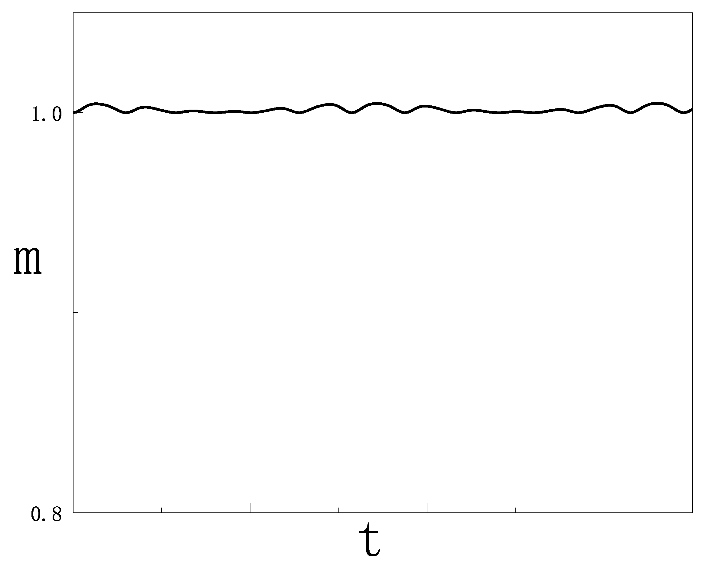
Figure 1.
Sketch of the corrected mass. The classical mass here is taken as .
Disclaimer/Publisher’s Note: The statements, opinions and data contained in all publications are solely those of the individual author(s) and contributor(s) and not of MDPI and/or the editor(s). MDPI and/or the editor(s) disclaim responsibility for any injury to people or property resulting from any ideas, methods, instructions or products referred to in the content. |
© 2023 by the authors. Licensee MDPI, Basel, Switzerland. This article is an open access article distributed under the terms and conditions of the Creative Commons Attribution (CC BY) license (https://creativecommons.org/licenses/by/4.0/).
Share and Cite
MDPI and ACS Style
Chen, Y.-J.; Li, S.-L.; Liu, Y.-Y.; Gu, X.; Li, W.-D.; Dai, W.-S. Model for Origin and Modification of Mass and Coupling Constant. Universe 2023, 9, 426. https://doi.org/10.3390/universe9090426
AMA Style
Chen Y-J, Li S-L, Liu Y-Y, Gu X, Li W-D, Dai W-S. Model for Origin and Modification of Mass and Coupling Constant. Universe. 2023; 9(9):426. https://doi.org/10.3390/universe9090426
Chicago/Turabian StyleChen, Yu-Jie, Shi-Lin Li, Yuan-Yuan Liu, Xin Gu, Wen-Du Li, and Wu-Sheng Dai. 2023. "Model for Origin and Modification of Mass and Coupling Constant" Universe 9, no. 9: 426. https://doi.org/10.3390/universe9090426
Note that from the first issue of 2016, this journal uses article numbers instead of page numbers. See further details here.