
Traveling Wave Solutions and Conservation Laws of a Generalized Chaffee–Infante Equation in (1+3) Dimensions
1
Department of Mathematical Sciences, University of South Africa (UNISA), Pretoria 0003, South Africa
2
Department of Mathematical Sciences, Mafikeng Campus, North-West University, Private Bag X2046, Mmabatho 2735, South Africa
3
Department of Mathematics, Faculty of Science, University of Botswana, Gaborone Private Bag 22, Botswana
*
Author to whom correspondence should be addressed.
Universe 2023, 9(5), 224; https://doi.org/10.3390/universe9050224
Submission received: 9 March 2023
/
Revised: 23 April 2023
/
Accepted: 5 May 2023
/
Published: 8 May 2023
(This article belongs to the Special Issue Mathematical Cosmology)
Abstract
:This paper aims to analyze a generalized Chaffee–Infante equation with power-law nonlinearity in (1+3) dimensions. Ansatz methods are utilized to provide topological and non-topological soliton solutions. Soliton solutions to nonlinear evolution equations have several practical applications, including plasma physics and the diffusion process, which is why they are becoming important. Additionally, it is shown that for certain values of the parameters, the power-law nonlinearity Chaffee–Infante equation allows solitons solutions. The requirements and restrictions for soliton solutions are also mentioned. Conservation laws are derived for the aforementioned equation. In order to comprehend the dynamics of the underlying model, we graphically show the secured findings. Hirota’s perturbation method is included in the multiple exp-function technique that results in multiple wave solutions that contain new general wave frequencies and phase shifts.
1. Introduction
Numerous physical phenomena, such as fluid mechanics, plasma waves, solid state physics, and plasma physics, are modeled through the theory of nonlinear evolution equations. The interactions between the nonlinear and dispersive elements of nonlinear partial differential equations lead to solitary waves, also known as solitons. Therefore, in order to have a comprehensive analysis of nonlinear partial differential equations, it is crucial to compute these types of solutions. There is no single approach for solving nonlinear partial differential equations, despite the fact that many efforts have been made in this direction, and conservation laws are crucial to the solution extraction process of nonlinear partial differential equations. Often, the initial step in solving a problem is to identify the conservation laws of a system of nonlinear partial differential equations. A system of nonlinear partial differential equations is said to be integrable if it has a significant number of conservation laws. Examples of such nonlinear evolution equations are the Sasa–Satsuma equations [1,2], nonlinear Schrodinger equations [3], and Korteweg–de Vries equations [4]. Therefore, finding closed-form solutions to these equations is essential. Since there is no one method for solving all NLEEs, several researchers have developed robust and efficient mathematical strategies to find closed-form solutions. A few of the main methods used to carry out the integration of NLEEs are the inverse Hirota’s bilinear approach [5,6], the tanh method [7,8], the Lie symmetry analysis method [7], the Darboux transformation method [9], and the Hirota bilinear method [10].
The nonlinear evolution equations depicted below [11,12]
are the Chaffee–Infante-type equations in (1+1) and (2+1) dimensions, respectively. They constitute reaction duffing equations that appear in mathematical physics [11]. The parameter adjusts the relative balance of the diffusion term and the nonlinear term and it should be noted that the above equations are also called Newell–Whitehead-type equations when [11]. The exp-function method was applied to (1) and (2) to generate traveling wave solutions in [12].
In this work, we study a generalized (1+3)-dimensional Chaffee–Infante equation with a power-law nonlinearity:
The Chaffee–Infante equation in (3+1) dimensions is a reaction diffusion equation that depicts high-energy physical processes, environmental science, and many other related areas of mathematical physics [13].
The parameters are real non-zero constants while the wave amplitude u is a function of the three scaled spatial variables and t the temporal variable. The term is the evolution term while is the nonlinear term with the power-law denoted by the exponent n, whereas the terms are the dispersions in the x-direction, y-direction, and z-direction, respectively.
This paper is organized into three sections. In Section 2, we apply a number of analytical methods to derive closed-form solutions to a power-law nonlinear Chaffee–Infante equation in (3+1) dimensions. There are three different soliton solutions: bright, dark, and singular. Section 3 deals with conservation laws of a Chaffee–Infante equation with (3+1) dimensions with the aid of a variational approach. Finally, in Section 4, we compute several waves of physical interest with innovative general wave frequencies and phase shifts via the multiple exp-function approach, which is a generalization of Hirota’s perturbation strategy.
2. Non-Topological Soliton Solutions
Several everyday occurrences must be understood using nonlinear evolution equations. In order to fully understand NLEEs, it is crucial to perform research and discover exact solutions to these equations. Nevertheless, integrating NLEEs is not always simple. Instead, the objective of this section is to use ansatz techniques to integrate Equation (3). We start by applying the following solitary wave ansatz:
so as to compute the one-soliton solution of Equation (3). Here the wave variable is denoted by :
where is the amplitude of the soliton, are the inverse widths of the soliton, is the velocity of the soliton, and finally p is a parameter to be determined. The utilization of Equations (3) and (4) leads to the following:
The exponents of and are equated in (6) so as to extract the least positive integer value of p. Consequentially, one attains:
which results in the following analytical condition:
Substituting on powers of and powers of in Equation (6) and thereafter setting the respective coefficients of powers of and powers of terms to zero leads to the following four algebraic systems of equations:
Solving the above systems yields:
Substituting the values of the wave amplitude , the soliton’s velocity , the inverse width , and the exponent p into Equation (4), we can determine the bright soliton or one-soliton solution of a generalized (2+1)-dimensional Chaffee–Infante Equation (3) as:
where the wave inverse widths are free parameters in this particular case.
It is important to note that the one-soliton solution for a generalized (2+1)-dimensional Chaffee–Infante Equation (3) only exists if , , and , while the inverse widths remain as free parameters. This important observation is being made for the first time to our knowledge. The evolution of the travelling wave solution (14) is given in Figure 1, Figure 2 and Figure 3.
2.1. Singular Soliton Solutions
Using two solitary wave ansatz approaches, we derive two single-soliton solutions in this subsection. The first hypothesis will take the form;
where the wave variable is given by:
where the parameter is the amplitude of the soliton, are the inverse widths of the soliton, and is the velocity of the soliton, whereas p is an unknown exponent. The values of these parameters are now unknown, and they will be established once the soliton solution of Equation (3) is derived. Employing Equations (3) and (15) gives rise to the following:
Now, equating the powers of and in (17) yields:
Upon solving the above equation we find that:
Substituting this value of p in (17), and thereafter equating the respective coefficients of powers of and powers of terms to zero, results in the following four algebraic systems of equations:
The solution for the unknown parameters is:
and:
As a result, the singular soliton solution for a (2+1)-dimensional Chaffe–Infante equation is:
with the wave widths and being free parameters.
It should be noted that a (3+1)-dimensional Chaffe–Infante equation possesses a singular soliton solution (26) if the elements fulfill the requirements , , and , although the inverse widths and remain free parameters. This is the first time that this observation has been recorded. A graphical simulation of the travelling wave solution (26) is given in Figure 4, Figure 5 and Figure 6.
The second solitary wave ansatz approach of the type
where the wave variable is defined as:
will be used to determine the second singular soliton solution of Equation (3).
We derive the following two cases for which Equation (3) permits a singular soliton solution by using the same approach as given above.
Case 1: , .
In this case, a (3+1)-dimensional Chaffe–Infante Equation (3) possesses a singular soliton solution of the form:
where:
Case 2: , .
Here, a (3+1)-dimensional Chaffe–Infante Equation (3) has a singular soliton solution of the form:
where:
It is important to note that a generalized (3+1) Chaffee–Infante equation does accept singular soliton solutions, but only if certain conditions are satisfied, including , , , and , while the inverse widths remain free parameters. Moreover, we note that Equation (3) has a second singular soliton solution if , , , and , while the inverse widths are left as free parameters. It should also be pointed out that there are no other values of the power-law nonlinearity element n for which singular soliton solutions will exist with respect to the function. This is a very commendable observation that is reported for the first time here and the graphical simulations of (29) and (31) is given in Figure 7, Figure 8 and Figure 9 and Figure 10, Figure 11 and Figure 12, respectively.
2.2. Dark Soliton Solution
This subsection aims to derive dark or shock wave soliton solutions for a generalized (3+1)-dimensional Chaffee–Infante Equation (3). In order to achieve this, we invoke the solitary wave ansatz hypothesis of the form [14]:
where the wave variable is defined as:
where symbolizes the soliton amplitude while are soliton inverse widths and is the velocity of the soliton, whereas p is an unknown exponent. Although these physical parameters in the soliton solution are unknown at this point, their exact values will be determined during the process of deriving the dark or topological soliton solution of Equation (3). Using Equation (33) and finding all the partial derivatives appearing in Equation (3) yields:
Inserting Equations (35)–(39) into Equation (3) gives:
We now equate the exponents of the and terms in Equation (41) in order to obtain the smallest positive integer value of p. Thus, we have:
which yields the following analytical condition:
Now, setting the respective coefficients of powers of terms to zero leads to the following seven algebraic systems of equations:
Solving these systems prompts the following cases for which Equation (3) admits dark soliton solutions.
Case 1: , .
In this case, a (3+1)-dimensional Chaffe–Infante Equation (3) has a dark soliton solution of the form:
where:
Case 2: , .
Here, a (3+1)-dimensional Chaffe–Infante Equation (3) admits a topological one-soliton solution of the form:
where:
The evolution of travelling wave solutions of (49) and (51) is given in Figure 13, Figure 14 and Figure 15 and Figure 16, Figure 17 and Figure 18, respectively.
Remark 1.
It is should be pointed out that dark soliton solutions for a generalized (3+1)-dimensional Chaffee–Infante Equation (3) do exists provided , , and , whereas the inverse widths remain free parameters. We further observe that Equation (3) admits a kink soliton solution if and only if , , , and , while the inverse width remains a free parameter. It is also shown that there are no other values of the power-law nonlinearity element n apart from and for which dark soliton solutions will exist associated with the function. This is a very crucial observation that is mentioned for the first time here.
3. Conservation Laws
This section aims to investigate conservation laws of a generalized Chaffee–Infante equation in (3+1) dimensions. Consider a differential equation , and being the characteristic function. is divergent if and only if , where is the Euler–Lagrange operator. Without loss of generality, we can now state the following theorems.
Theorem 1.
A generalized Chaffee–Infante equation in (3+1) dimensions (3) formally admits a unique characteristic function, namely:
where satifies .
Proof.
A straightforward but lengthy computation can be carried out from . The expansion of this equation leads to an over-determined system of linear differential equations in the unknown characteristic function . Solving these equations, one obtains the unique characteristic function (53). □
The existence of this characteristic function prompts the following theorem.
Theorem 2.
A generalized Chaffee–Infante equation in (3+1) dimensions (3) strictly admits an infinite set of conservation laws corresponding to the unique characteristics , namely:
respectively.
Proof.
The proof of Theorem 2 is straightforward but long. It consists of applying the divergence equation , which vanishes for all solutions of a generalized Chaffee–Infante equation in (3+1) dimensions (3), whenever satisfies □
It is important to note that a generalized Chaffee–Infante equation in (3+1) dimensions (3) technically does not accept any conservation laws when the power-law index . Conservation laws are mathematical representations that when investigated illustrate a plethora of physical phenomena such as energy, mass momentum, angular momentum, and other physical quantities. A careful observation of these conservation laws indicates that they represent conservation of energy and momentum whenever the arbitrary function is set to be constant.
4. Multiple Exp-Function Method
In this section, the multiple exp-function approach that involves the following steps is shown:
Step 1. Defining differential equations that can be solved
Consider a partial differential equation in the scalar (1+1) dimensions:
We introduce several new variables in succession: , , and PDEs that can be solved, such as the linear ones:
where , are the angular wave numbers and , are the wave frequencies. It should be noted that solving such linear equations yields the solutions of the exponential function and that this is frequently the first step in creating exact solutions to nonlinear partial differential equations:
where and are arbitrary constants.
Step 2. Nonlinear PDE transformation
Consider rational solutions in the new variables , :
where and are all constants to be determined from the original Equation (54). By manipulating differential relations in (55), we can express all partial derivatives of u with x and t in terms of , . For example, we can have:
and:
where and are partial derivatives of and with respect to . Substituting (57) and its derivatives leads to a rational function equation with the new variables , :
This is called the transformed equation of the original Equation (54).
Step 3. Solving algebraic systems
Now, we set the numerator of the resulting rational function to zero. This yields a system of algebraic equations of all variables . We solve this system to determine the two polynomials and and the wave exponents , . As a result, the multiple wave solution u is computed and given by:
4.1. Application of the Multiple Exp-Function Method to (3)
We will use the multiple exp-function method in this subsection to obtain one-, two-, and three-wave solutions of (3). Phase shifts and general wave frequencies are included in the solutions that follow.
4.1.1. One-Wave Solution of (3)
Employing multiple exp-function method as outlined in Section 2, we find that the desired one-wave solution is of the form:
where
4.1.2. Two-Wave Solution of (3)
The intended two-wave solution, as determined by the multiple exp-function approach described in Section 2, has the following two forms as depicted below:
CASE I
CASE II
4.1.3. Three-Wave Solution of (3)
The multiple exp-function method outlined in Section 2 is used to determine the anticipated two-wave solution, which takes the following five forms as depicted in the ensuing cases:
CASE I
CASE II
CASE III
CASE IV
CASE V
It should be pointed out that the above traveling wave solutions can also be written in terms of hyperbolic functions.
5. Concluding Remarks
The purpose of this research was to investigate a generalized the Chaffee–Infante equation in (1+3) dimensions with power-law nonlinearity. To create topological and non-topological soliton solutions, ansatz approaches were used. Additionally, it was shown that the power-law nonlinearity Chaffee–Infante equation permits solitons solutions for certain values of the parameters. Infinitely many conservation laws were computed. Finally, the underlying model’s multiple wave solutions were built using the multiple exp-function approach, which is a generalization of Hirota’s perturbation strategy that yielded novel general wave frequencies and phase shifts. The techniques employed in this research to find novel precise solutions may also be used for the solution of other nonlinear partial differential equations of physical importance. The methods presented in this paper are crucial for certain significant classical mathematical and physical models. The exact solutions found in this work may be compared to numerical simulations in theoretical physics and fluid mechanics, and the conservation laws found can be used to build numerical integrators for the system at hand.
Author Contributions
Conceptualization, M.C.S., Conceptualization, B.M., Conceptualization, A.R.A. All authors have read and agreed to the published version of the manuscript.
Funding
This research received no external funding.
Data Availability Statement
All data generated or analyzed during this study are included in this manuscript.
Acknowledgments
Motshidisi Charity Sebogodi would like to thank the SA-UK USDP program for their financial support and their research development programs.
Conflicts of Interest
The authors declare no conflict of interest.
References
- Ma, W. Sasa-Satsuma type matrix integrable hierarchies and their Riemann–Hilbert problems and soliton solutions. Phys. D Nonlinear Phenom. 2023, 446, 133672. [Google Scholar] [CrossRef]
- Liu, Y.; Zhang, W.; Ma, W. Riemann-Hilbert problems and soliton solutions for a generalized coupled Sasa-Satsuma equation. Commun. Nonlinear Sci. Numer. Simul. 2023, 118, 107052. [Google Scholar] [CrossRef]
- Ma, W. Soliton solutions to constrained nonlocal integrable nonlinear Schrödinger hierarchies of type (−λ, λ). Int. J. Geom. Methods Mod. Phys. 2023, 7, 100515. [Google Scholar]
- Ma, W. Matrix integrable fifth-order mKdV equations and their soliton solutions. Chin. Phys. B 2023, 32, 020201. [Google Scholar] [CrossRef]
- Chen, S.; Lü, X. Observation of resonant solitons and associated integrable properties for nonlinear waves. Chaos Solitons Fractals 2022, 163, 112543. [Google Scholar] [CrossRef]
- He, X.-J.; Lü, X. M-lump solution, soliton solution and rational solution to a (3+1)-dimensional nonlinear model. Math. Comput. Simul. 2022, 197, 327–340. [Google Scholar] [CrossRef]
- Adem, A. Symbolic computation on exact solutions of a coupled Kadomtsev–Petviashvili equation: Lie symmetry analysis and extended tanh method. Comput. Math. Appl. 2017, 74, 1897–1902. [Google Scholar] [CrossRef]
- Muatjetjeja, B.; Adem, A. Rosenau-KdV equation coupling with the Rosenau-RLW equation: Conservation laws and exact solutions. Int. J. Nonlinear Sci. Numer. Simul. 2017, 18, 451–456. [Google Scholar] [CrossRef]
- Ye, R.; Zhang, Y.; Ma, W. Darboux transformation and dark vector soliton solutions for complex mKdV systems. Part. Differ. Equ. Appl. Math. 2021, 4, 100161. [Google Scholar] [CrossRef]
- Ma, W. Soliton solutions by means of Hirota bilinear forms. Part. Differ. Equ. Appl. Math. 2022, 5, 100220. [Google Scholar] [CrossRef]
- Constantin, P.; Foias, C.; Nicolaenko, B.; Temam, R. Integral Manifolds and Inertial Manifolds for Dissipative Partial Differential Equations; Springer: Berlin/Heidelberg, Germany, 1989. [Google Scholar]
- Sakthivel, R.; Chun, C. New soliton solutions of Chaffee-Infante equations using the exp-function method. Z. Naturforsch.-Sect. A J. Phys. Sci. 2010, 65, 197–202. [Google Scholar] [CrossRef]
- Mao, Y. Exact solutions to (2+1)-dimensional Chaffee–Infante equation. Pramana-J. Phys. 2018, 91, 9. [Google Scholar] [CrossRef]
- Wazwaz, A. New compactons, solitons and periodic solutions for nonlinear variants of the KdV and the KP equations. Chaos Solitons Fractals 2004, 22, 249–260. [Google Scholar] [CrossRef]
Figure 1.
A 3D profile structure of Solution (14) with parameters , .
Figure 1.
A 3D profile structure of Solution (14) with parameters , .
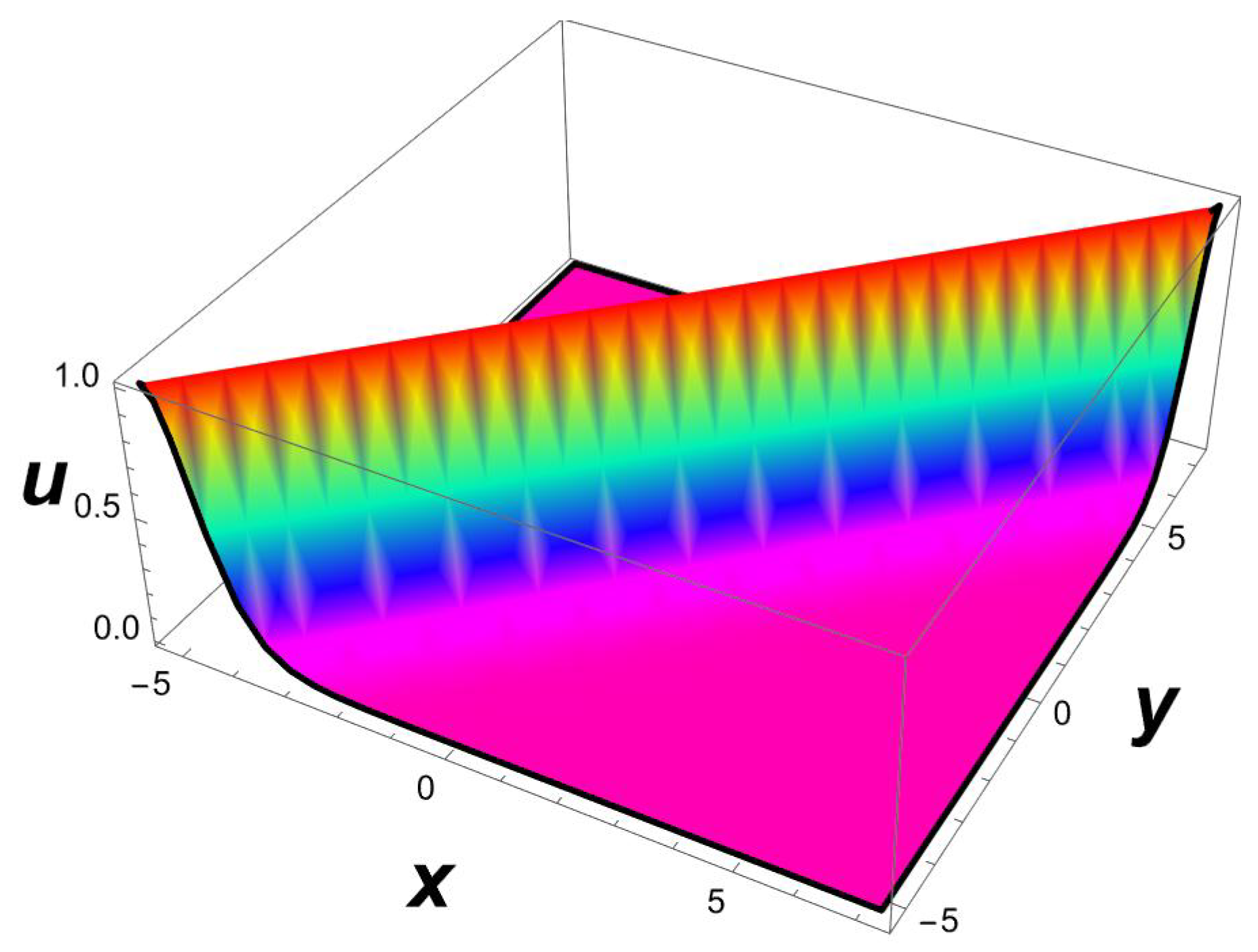
Figure 2.
A 2D side view of Figure 1.
Figure 2.
A 2D side view of Figure 1.
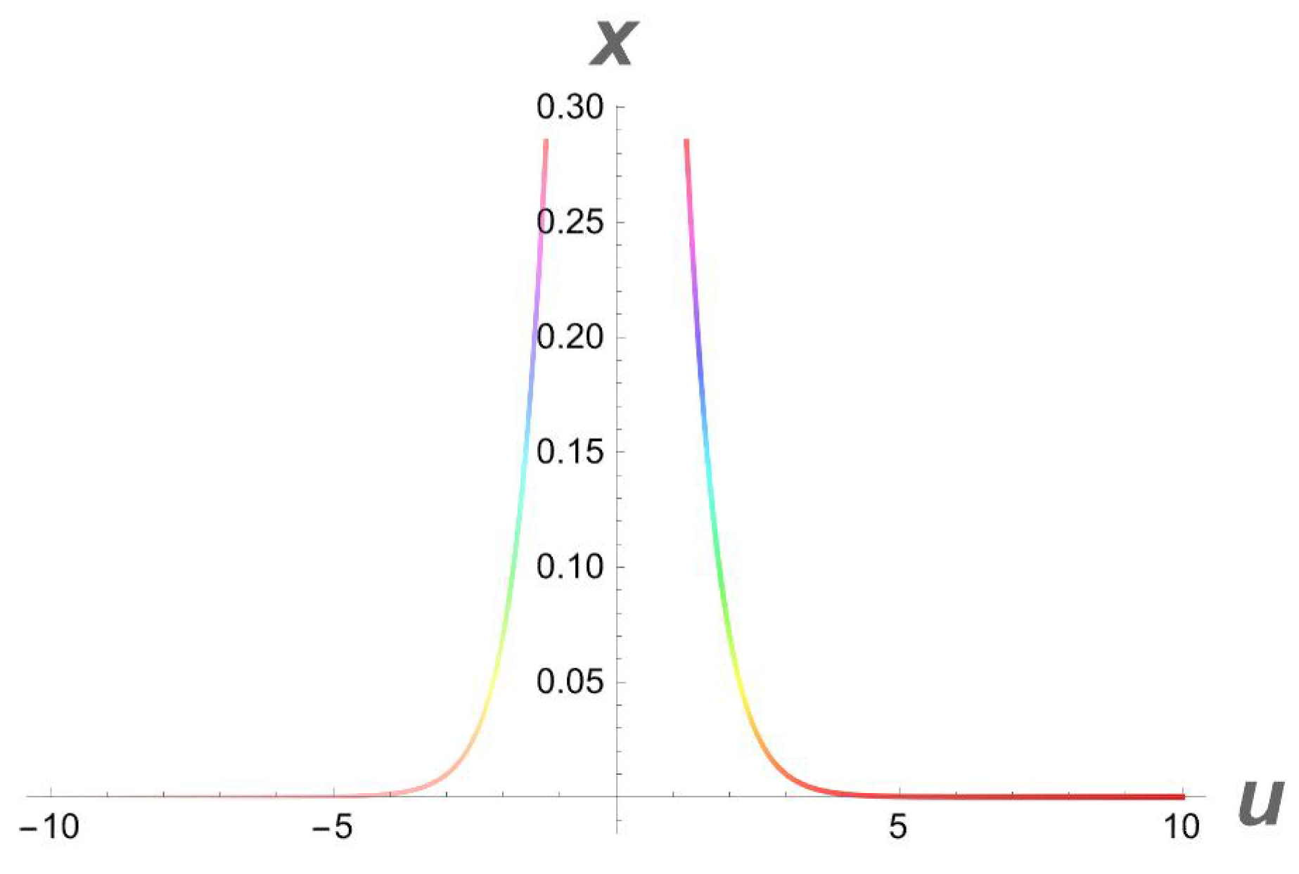
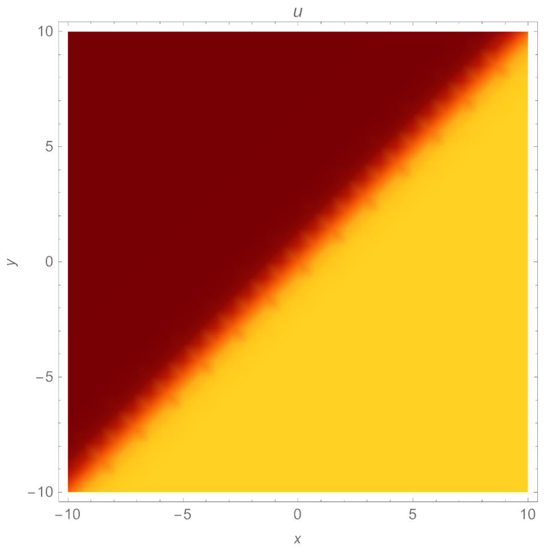
Figure 3.
A density plot of non-topological soliton of (14) with parameters , .
Figure 3.
A density plot of non-topological soliton of (14) with parameters , .
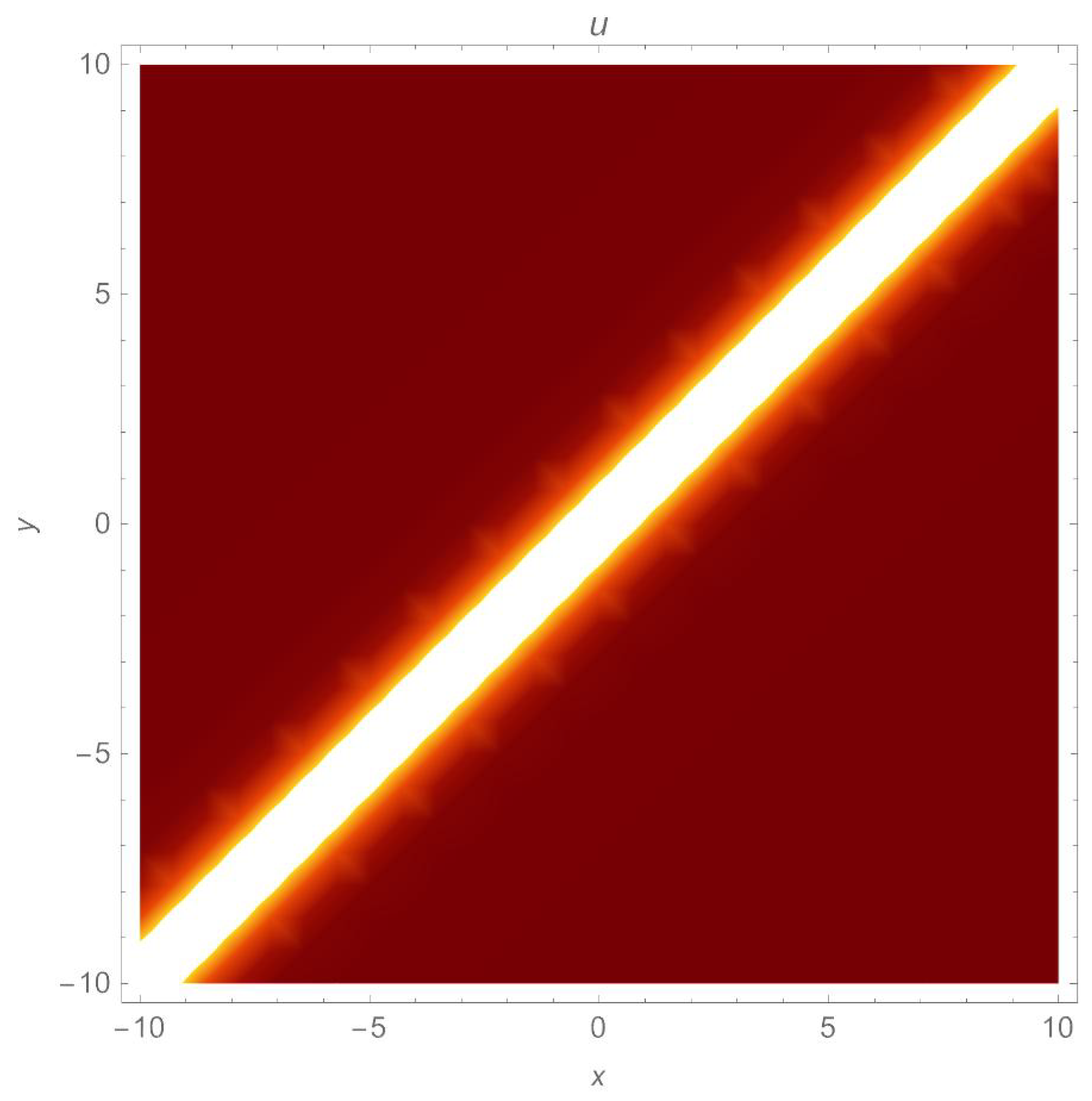
Figure 4.
A 3D profile structure of a singular soliton (26) with parameters , .
Figure 4.
A 3D profile structure of a singular soliton (26) with parameters , .
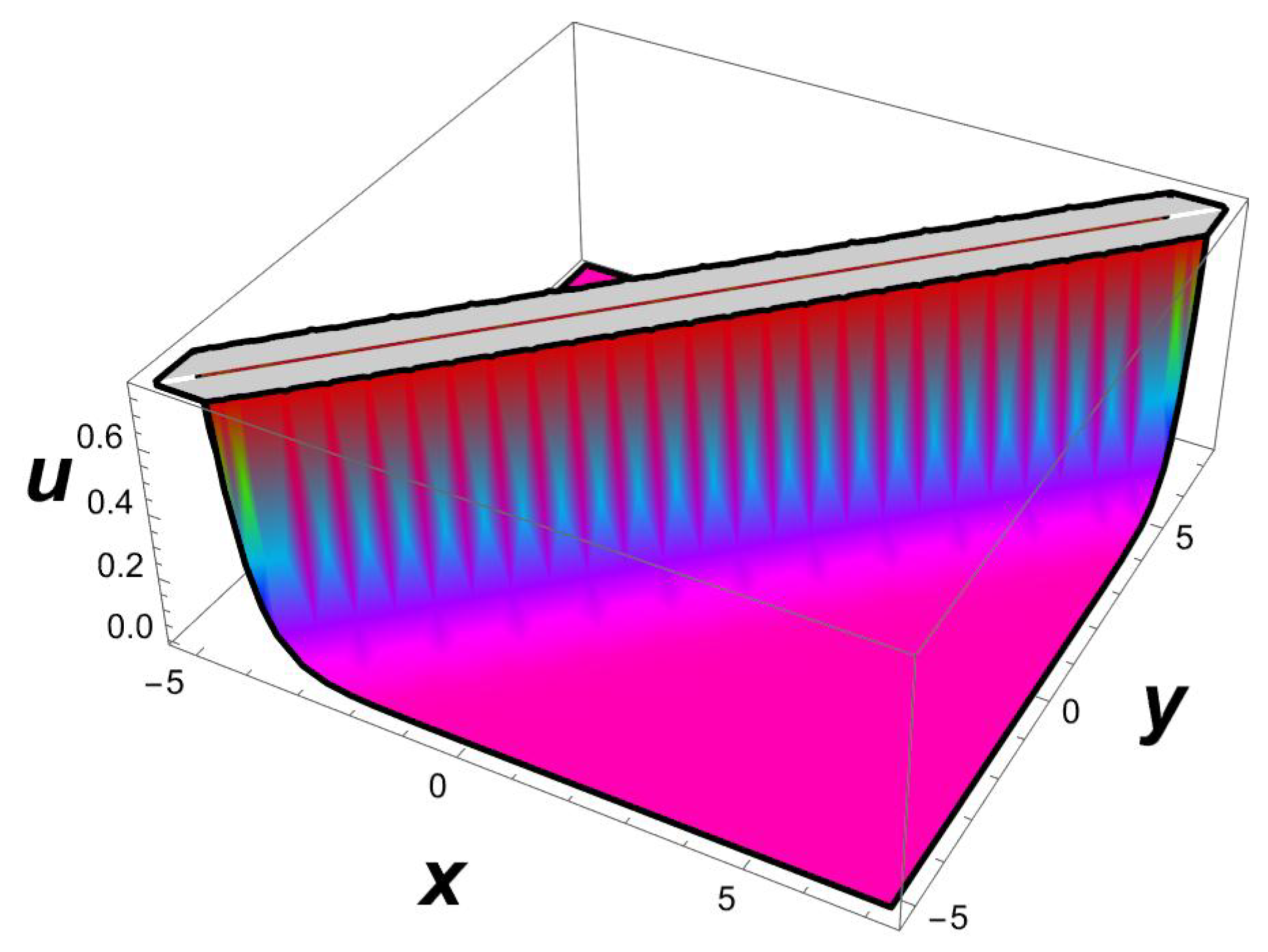
Figure 5.
A 2D side view of Figure 4.
Figure 5.
A 2D side view of Figure 4.
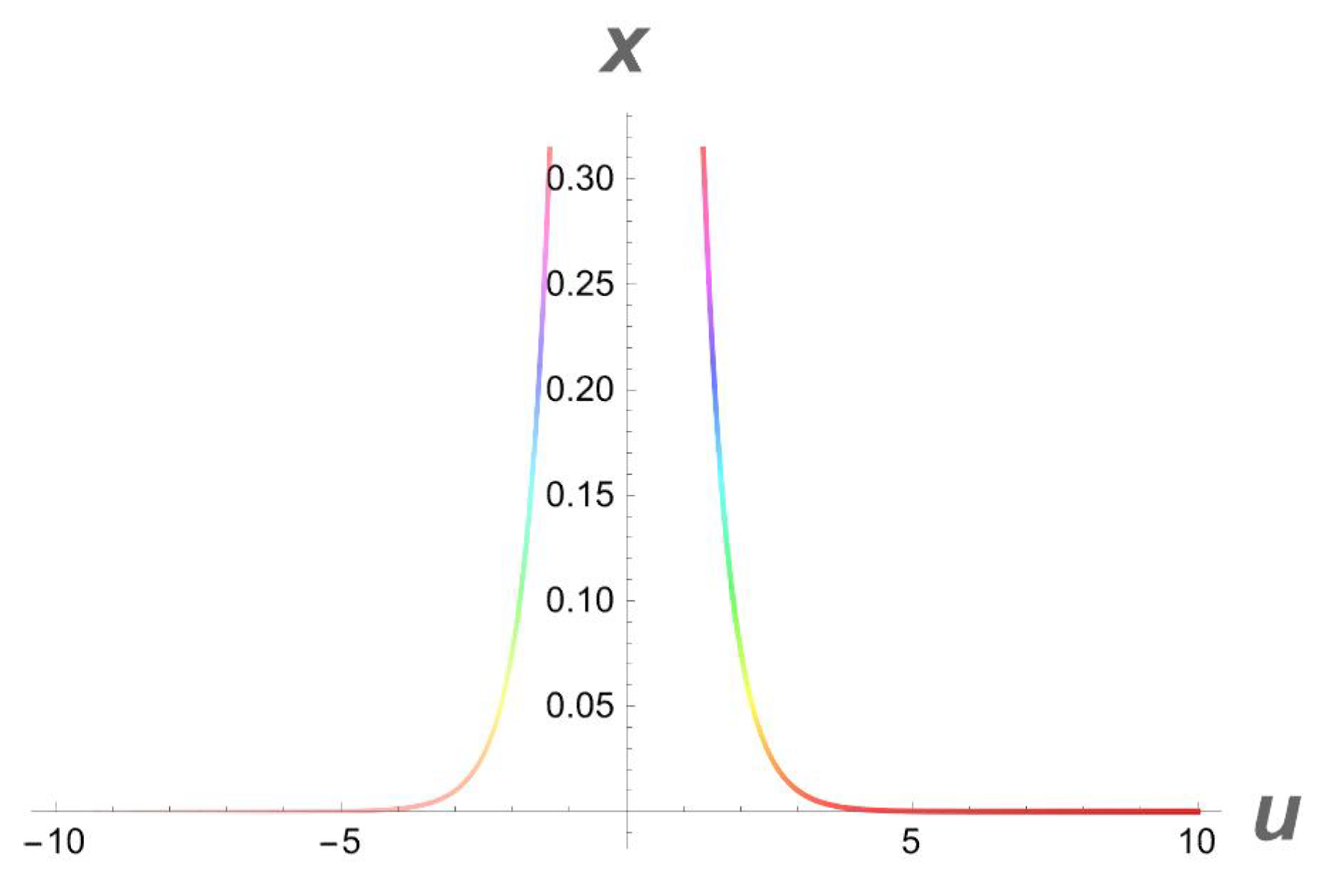
Figure 6.
A density plot of a singular soliton (26) with parameters , .
Figure 6.
A density plot of a singular soliton (26) with parameters , .
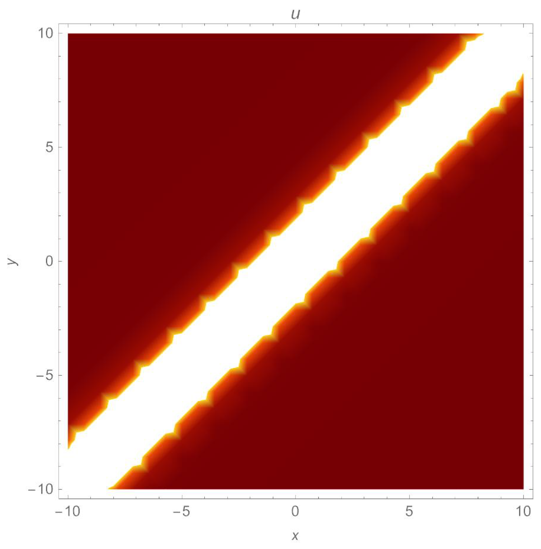
Figure 7.
A 3D profile of a singular soliton (29) with parameters , .
Figure 7.
A 3D profile of a singular soliton (29) with parameters , .
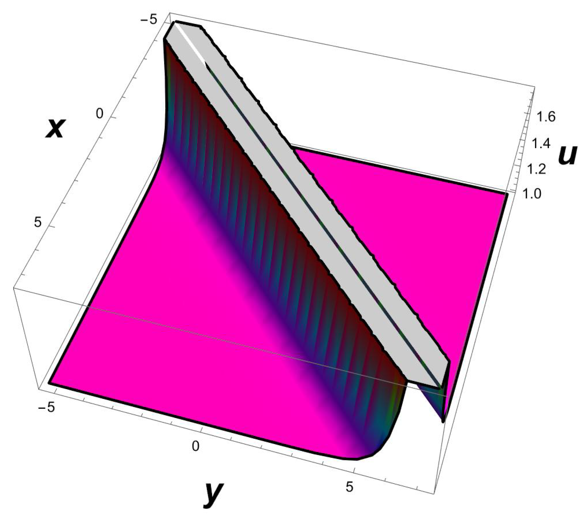
Figure 8.
A 2D side view of Figure 7.
Figure 8.
A 2D side view of Figure 7.
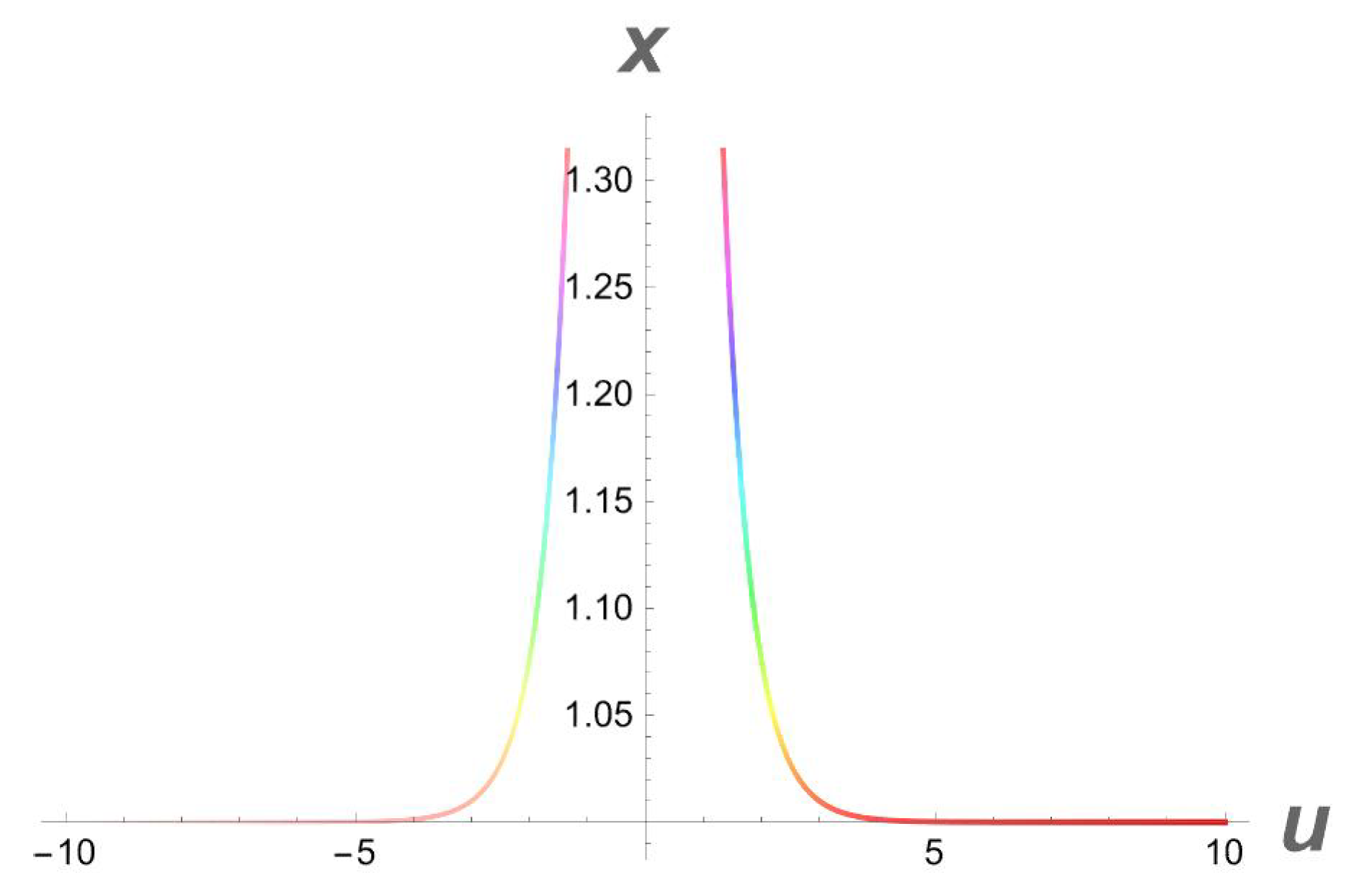
Figure 9.
A density plot of a singular soliton (29) with parameters , .
Figure 9.
A density plot of a singular soliton (29) with parameters , .
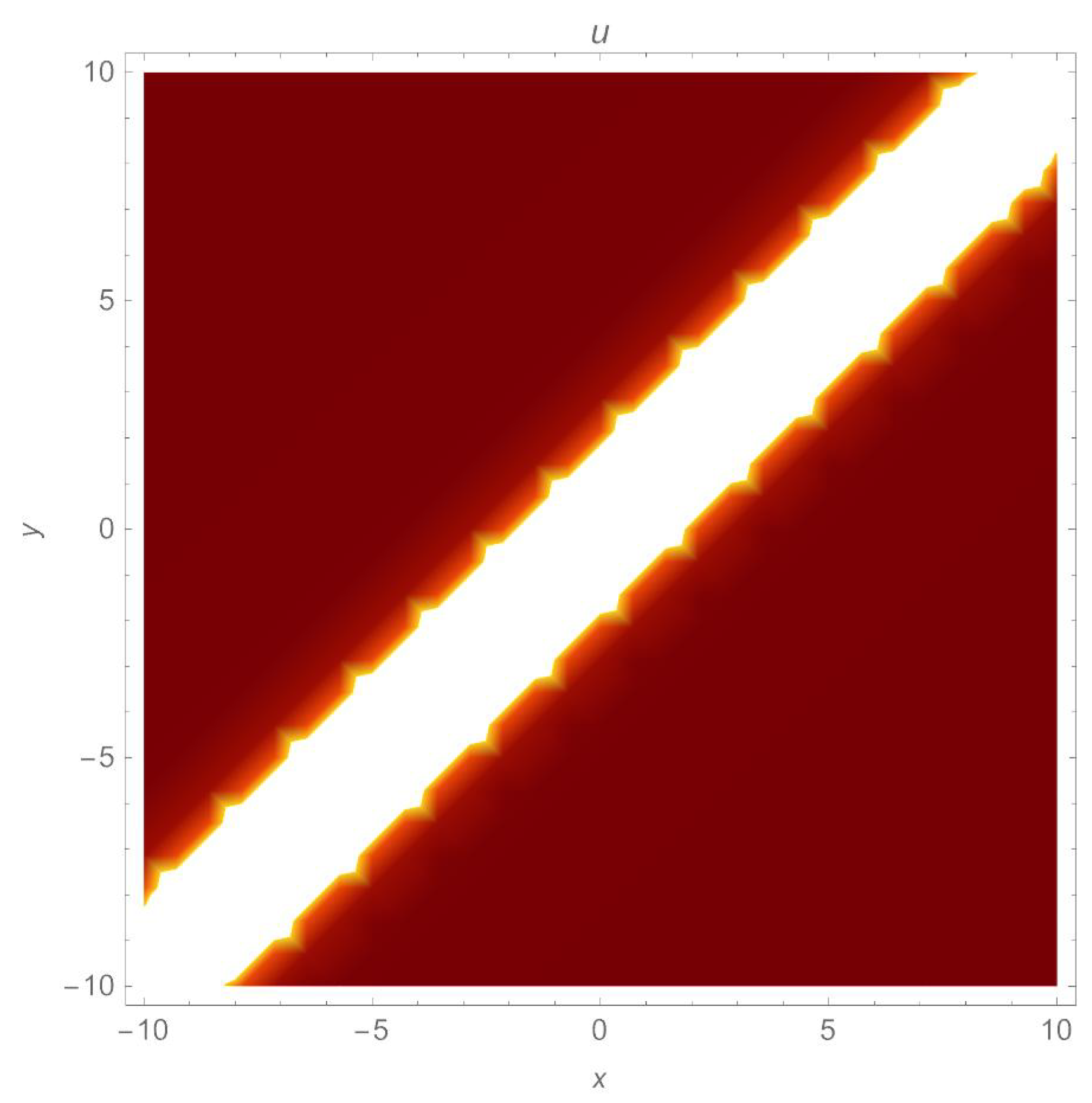
Figure 10.
A 3D profile of a singular soliton (31) with parameters , .
Figure 10.
A 3D profile of a singular soliton (31) with parameters , .
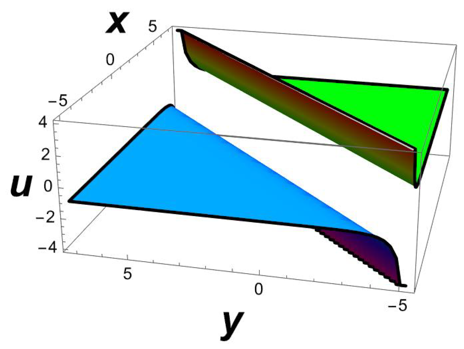
Figure 11.
A 2D side view of Figure 10.
Figure 11.
A 2D side view of Figure 10.
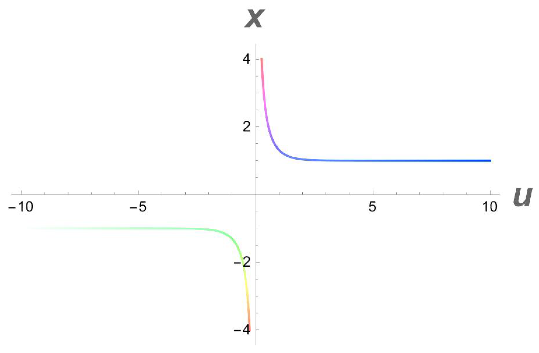
Figure 12.
A density plot of the periodic structure of a singular soliton (31) with parameters , .
Figure 12.
A density plot of the periodic structure of a singular soliton (31) with parameters , .
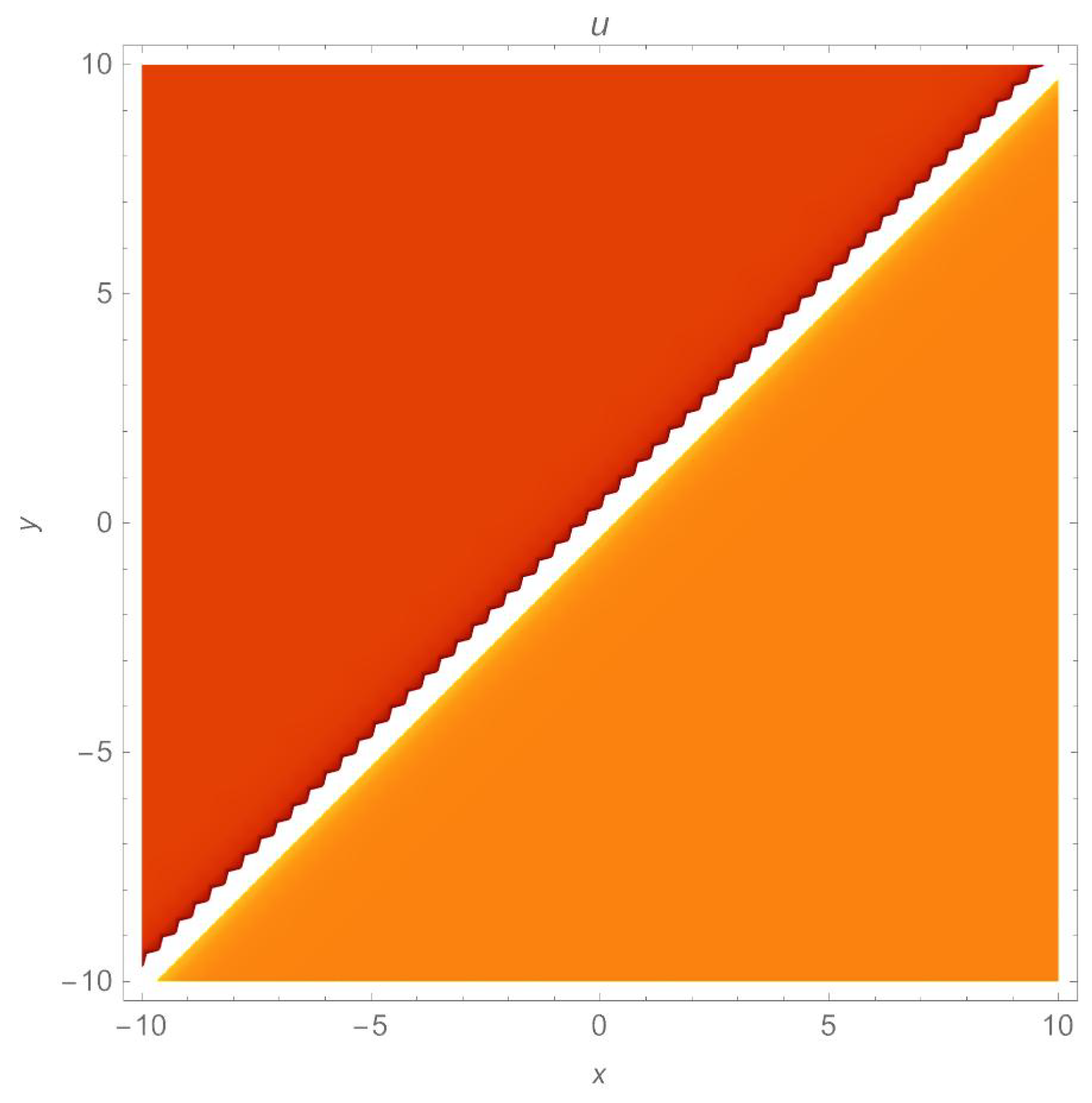
Figure 13.
A 3D profile structure of a dark soliton solution (49) with parameters , .
Figure 13.
A 3D profile structure of a dark soliton solution (49) with parameters , .
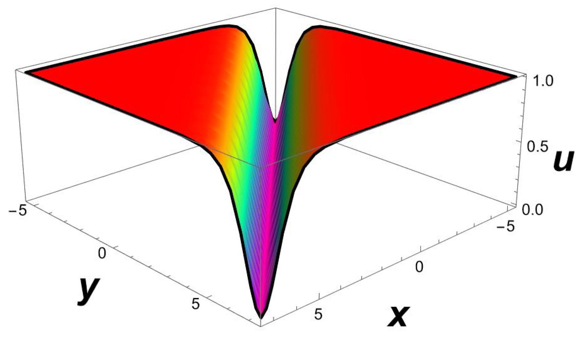
Figure 14.
A 2D side view of Figure 13.
Figure 14.
A 2D side view of Figure 13.
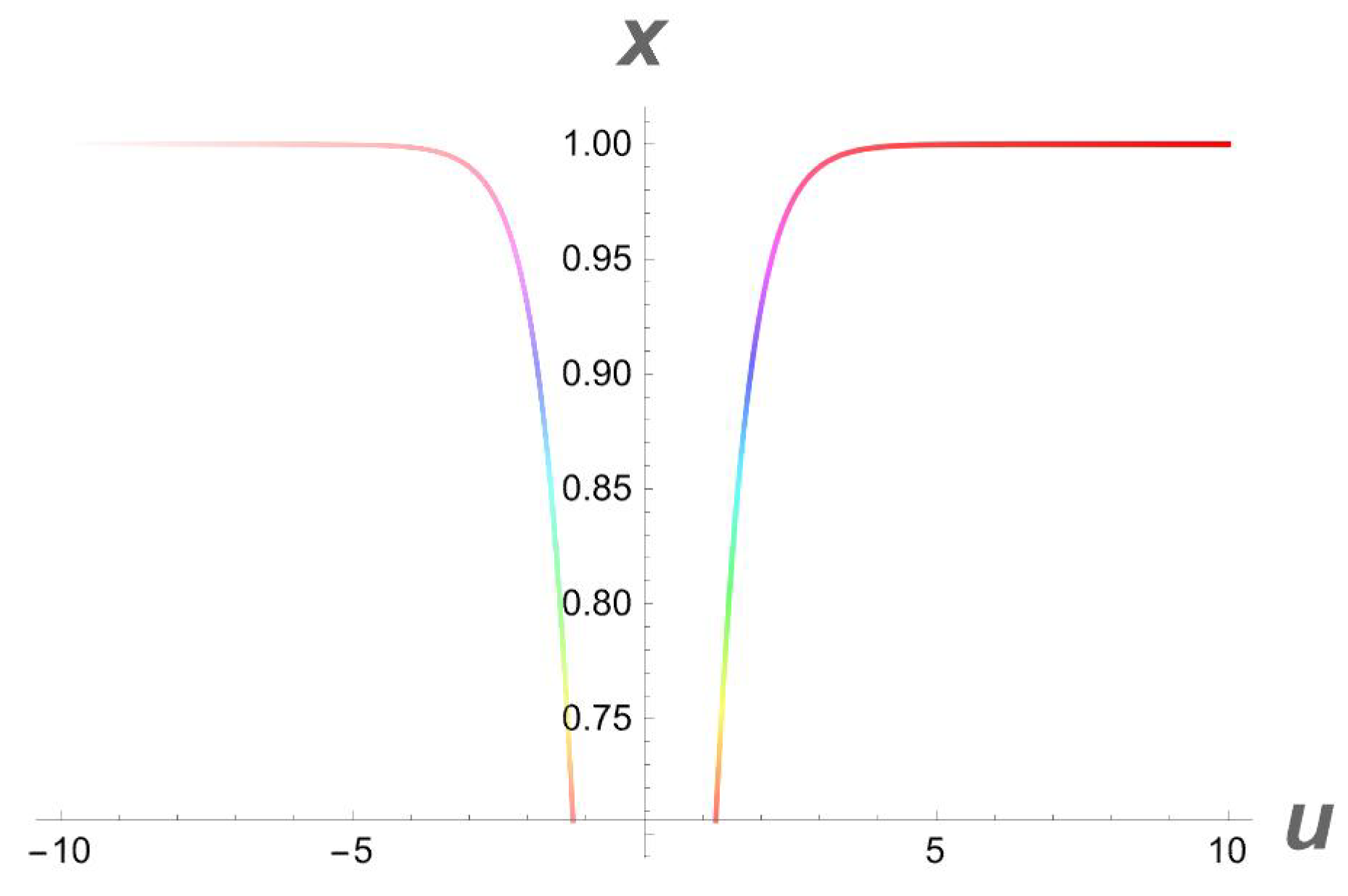
Figure 15.
A density plot of a dark soliton solution (49) with parameters , .
Figure 15.
A density plot of a dark soliton solution (49) with parameters , .

Figure 16.
A 3D profile structure of a dark soliton solution (51) with parameters , .
Figure 16.
A 3D profile structure of a dark soliton solution (51) with parameters , .
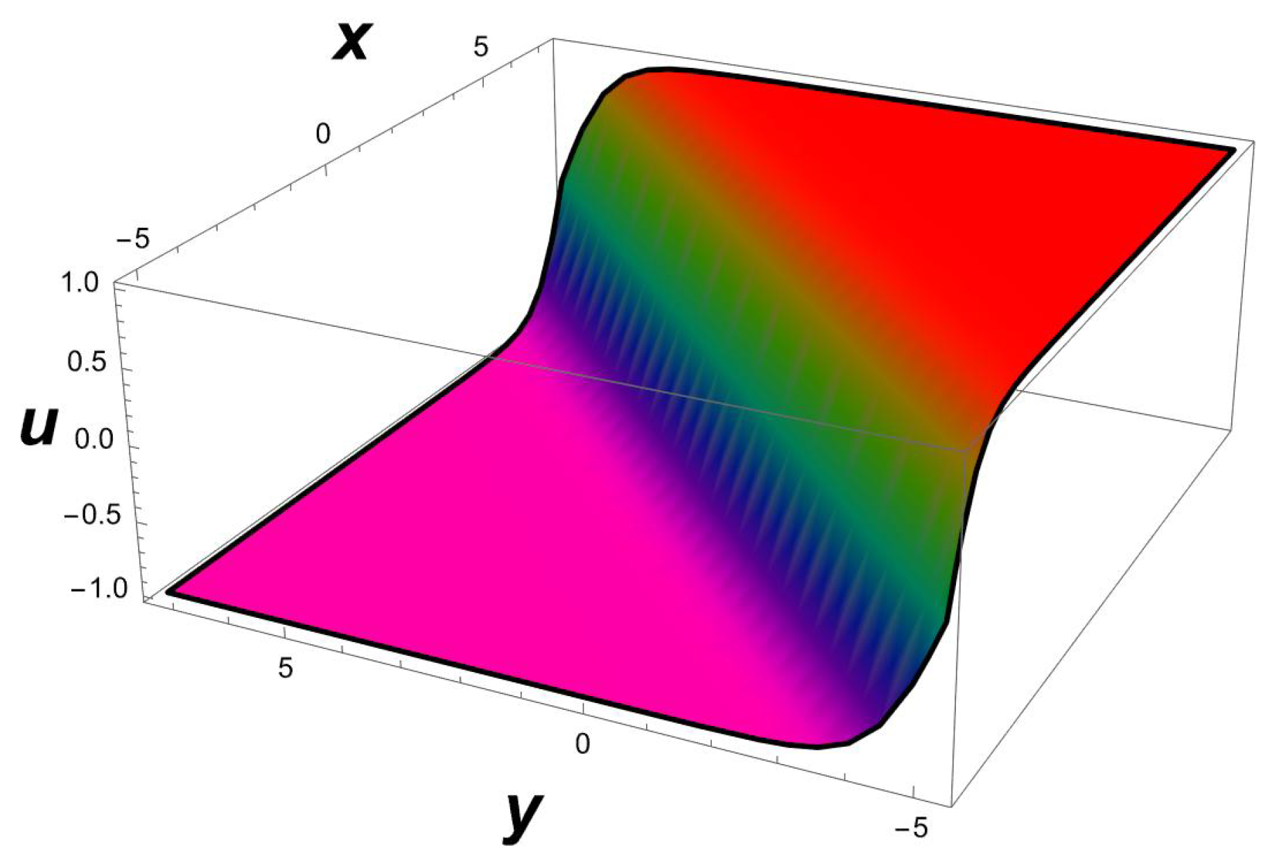
Figure 17.
A 2D side view of Figure 16.
Figure 17.
A 2D side view of Figure 16.
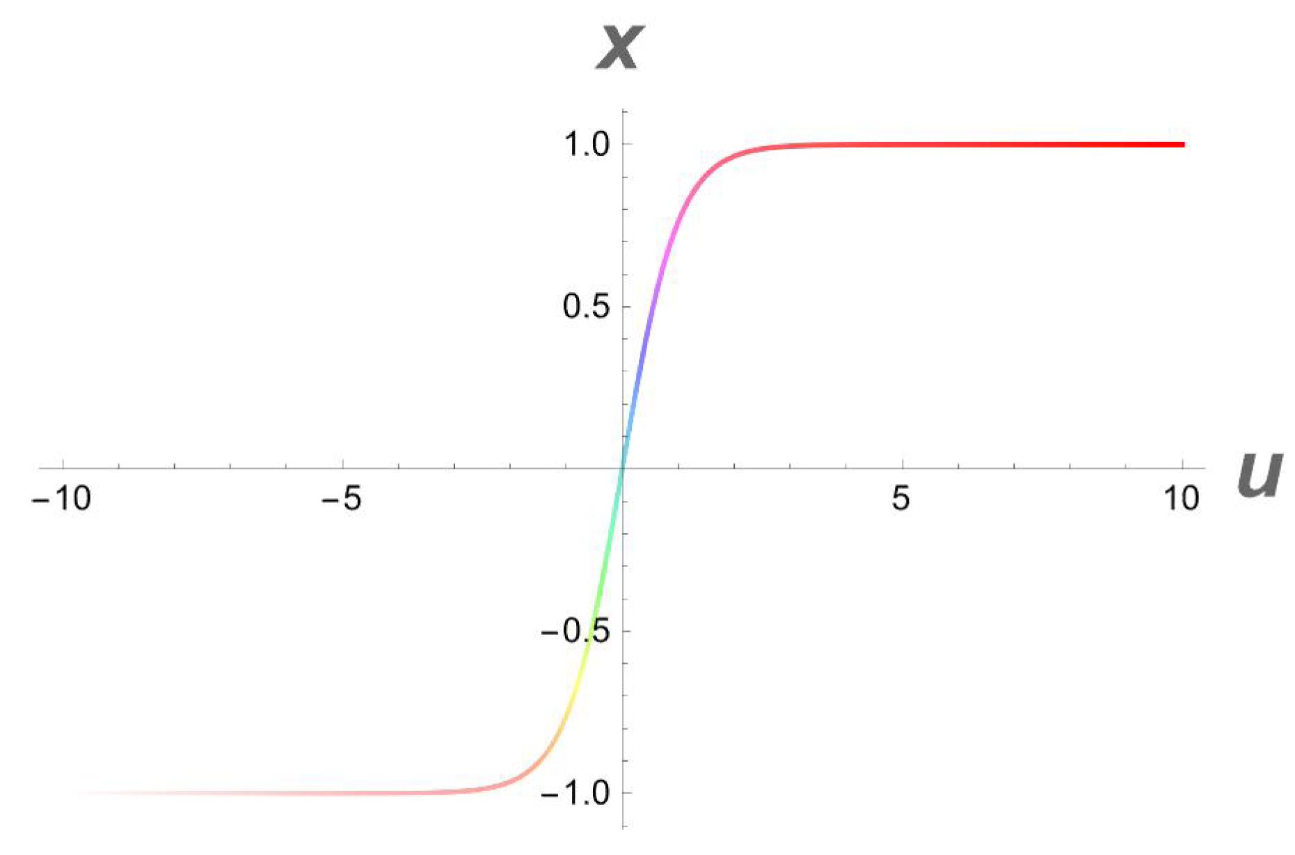
Figure 18.
A density plot of a dark soliton solution (51) with parameters .
Figure 18.
A density plot of a dark soliton solution (51) with parameters .
Disclaimer/Publisher’s Note: The statements, opinions and data contained in all publications are solely those of the individual author(s) and contributor(s) and not of MDPI and/or the editor(s). MDPI and/or the editor(s) disclaim responsibility for any injury to people or property resulting from any ideas, methods, instructions or products referred to in the content. |
© 2023 by the authors. Licensee MDPI, Basel, Switzerland. This article is an open access article distributed under the terms and conditions of the Creative Commons Attribution (CC BY) license (https://creativecommons.org/licenses/by/4.0/).
Share and Cite
MDPI and ACS Style
Sebogodi, M.C.; Muatjetjeja, B.; Adem, A.R. Traveling Wave Solutions and Conservation Laws of a Generalized Chaffee–Infante Equation in (1+3) Dimensions. Universe 2023, 9, 224. https://doi.org/10.3390/universe9050224
AMA Style
Sebogodi MC, Muatjetjeja B, Adem AR. Traveling Wave Solutions and Conservation Laws of a Generalized Chaffee–Infante Equation in (1+3) Dimensions. Universe. 2023; 9(5):224. https://doi.org/10.3390/universe9050224
Chicago/Turabian StyleSebogodi, Motshidisi Charity, Ben Muatjetjeja, and Abdullahi Rashid Adem. 2023. "Traveling Wave Solutions and Conservation Laws of a Generalized Chaffee–Infante Equation in (1+3) Dimensions" Universe 9, no. 5: 224. https://doi.org/10.3390/universe9050224
Note that from the first issue of 2016, this journal uses article numbers instead of page numbers. See further details here.