Cosmic Inflation, Quantum Information and the Pioneering Role of John S Bell in Cosmology

Simple Summary

I discuss whether a signature of the quantum origin of large scale structures observed in our Universe can be found.

Abstract

According to the theory of cosmic inflation, the large scale structures observed in our Universe (galaxies, clusters of galaxies, Cosmic Background Microwave—CMB—anisotropy…) are of quantum mechanical origin. They are nothing but vacuum fluctuations, stretched to cosmological scales by the cosmic expansion and amplified by gravitational instability. At the end of inflation, these perturbations are placed in a two-mode squeezed state with the strongest squeezing ever produced in Nature (much larger than anything that can be made in the laboratory on Earth). This article studies whether astrophysical observations could unambiguously reveal this quantum origin by borrowing ideas from quantum information theory. It is argued that some of the tools needed to carry out this task have been discussed long ago by J. Bell in a, so far, largely unrecognized contribution. A detailled study of his paper and of the criticisms that have been put forward against his work is presented. Although J. Bell could not have realized it when he wrote his letter since the quantum state of cosmological perturbations was not yet fully characterized at that time, it is also shown that Cosmology and cosmic inflation represent the most interesting frameworks to apply the concepts he investigated. This confirms that cosmic inflation is not only a successful paradigm to understand the early Universe. It is also the only situation in Physics where one crucially needs General Relativity and Quantum Mechanics to derive the predictions of a theory and, where, at the same time, we have high-accuracy data to test these predictions, making inflation a playground of utmost importance to discuss foundational issues in Quantum Mechanics.

1. Introduction

The theory of cosmic inflation [1,2,3,4,5,6] is considered as the leading paradigm for describing the physical conditions that prevailed in the early Universe. It is a very successful theory because it solves the puzzles of the standard model of Cosmology, but, also, because it has made predictions that have been observationally verified (for a recent assessment of the scientific status of inflation—see Refs. [7,8]). For instance, it predicts the presence of Doppler peaks in the Cosmic Microwave Background (CMB) multipoles’ moments, a vanishing spatial curvature or a power spectrum of cosmological perturbations close to scale invariance but not exactly scale invariant [9,10,11,12,13,14] (for reviews, see e.g., Refs. [15,16]). This last prediction has been verified, at a statistical significant level, only recently, thanks to the release of the European Space Agency (ESA) satellite Planck data [17,18,19,20,21].

However, inflation is also interesting because it combines Quantum Mechanics and General Relativity. Indeed, according to inflation, all structures in our Universe are of quantum-mechanical origin. This claim, although very strong, seems to be empirically correct in the sense that all conclusions that can be derived from this assumption fit well the data at our disposal. However, it would clearly be interesting to go beyond an indirect proof and to be able to find an explicit and unambiguous signature of the quantum origin of the structures present in our Universe.

This article is devoted to this question and discusses the tools, often borrowed to Quantum Information Theory, that can be used in order to address these problems [22,23,24,25,26].

We also argue that crucial insights into those issues were anticipated by John Bell in a, so far, unrecognized contribution “EPR correlations and EPW distributions” [27] reproduced in his book “Speakable and unspeakable in quantum mechanics” [28]. This letter was written after the invention of inflation but before the quantum state of cosmological perturbations was fully characterized by Grishchuk and Sidorov [29]. It discusses important ideas related to the classical limit of Quantum Mechanics. We study Bell’s paper but also the criticisms that have been put forward against it [30]. There was indeed a long and controversial discussion about the validity of the results obtained by Bell. What was not realized before, however, is that the domains most applicable to the ideas developed by Bell in his article are Cosmology and the scenario of cosmic inflation.

The article is organized as follows. In the next section, Section 2, we first review the theory of inflationary cosmological perturbations, at the classical level in Section 2.1 and, then, in Section 2.2 at the quantum level. In Section 2.3, we study in more detail the quantum state in which inflationary perturbations are placed, namely a two-mode squeezed state. In Section 2.4, we present some simple considerations that allow us to intuitively understand what a squeezed state is and, in Section 2.5, we show that these types of states, in fact, belong to a larger class of quantum states known as Gaussian states. In Section 3, we study the quantum-to-classical transition of cosmological perturbations. In Section 3.1, we investigate if the fluctuations can be described by a classical stochastic process. In Section 3.2, we use tools borrowed from quantum information theory, namely the quantum discord, to address the question of the classicality of cosmological perturbations. In Section 4, we come back again to the question of the classical limit using Bell ideas. In Section 4.1, we explain why the non-positivity of the Wigner function can be taken as a criterion for the existence of genuine quantum effects. In Section 4.2, we discuss this idea in the context of the Wentzel–Kramer–Brillouin (WKB) approximation. In Section 4.3, we review in detail the paper by John Bell, mentioned earlier, and show that it is especially relevant for our purposes. In Section 4.4, we present the criticisms that have been made on Bell’s letter and, in Section 4.5, we comment on these criticisms. In Section 4.6, in the light of the previous considerations, we conclude about the status of Bell’s letter. Finally, in Section 4.7, we explain how the whole situation has been clarified by the publication of a theorem due to Revzen. In Section 5, based on the previous considerations, we study whether the Bell inequality can be constructed for CMB observables and we briefly discuss our results in Section 6. Finally, in Section 7, we briefly present our conclusions.

2. Inflationary Cosmological Perturbations

2.1. Classical Perturbations

On large scales, the Universe is homogeneous and isotropic (the so-called cosmological principle) and is well-described by the Friedman–Lemaître–Robertson–Walker (FLRW) metric, $\mathrm{d}{s}^2=a^2\left(\eta \right)(-\mathrm{d}{\eta }^2+{\delta }_{ij}\mathrm{d}{x}^i\mathrm{d}{x}^j)$, where $\eta$ is the conformal time and $a\left(\eta \right)$ the scale factor. The scale factor describes how the Universe expands. We now have an accurate picture of the behavior of $a\left(\eta \right)$ from epochs possibly characterized by an energy scale as high as ~${10}^{15}$ GeV to present times. This cosmic history constitutes the standard model of Cosmology, known as the ΛCDM model [31]. This model is a six parameter model and correctly accounts for all known cosmological observations. The earliest epoch of this ΛCDM model, namely the one which describes the very early Universe, is known as inflation. It is a phase of accelerated expansion and it is believed that it was driven by a scalar field, the “inflaton”, the physical nature of which is still unknown.

However, in order to understand the large scale structures in our Universe, such as clusters of galaxies or CMB anisotropies, it is clearly necessary to go beyond the previous description, namely beyond the cosmological principle. A crucial remark is that, in the early Universe, the deviations from homogeneity and isotropy are small (recall that $\delta T/T~{10}^{-5}$ on the last scattering surface). As a consequence, one can use perturbative methods: as a matter of fact, linear perturbations theory will be sufficient. Therefore, we perturb the FLRW metric tensor introduced before and write [32] $g_{\mu \nu }=g_{\mu \nu }^{\mathrm{FLRW}}\left(\eta \right)+\delta g_{\mu \nu }(\eta ,\mathit{x})+\cdots$, where $g_{\mu \nu }^{\mathrm{FLRW}}\left(\eta \right)$ is the metric tensor introduced before which only depends on time since it describes a homogeneous and isotropic Universe. The perturbed part is $\delta g_{\mu \nu }(\eta ,\mathit{x})$, which is supposed to be small compared to $g_{\mu \nu }^{\mathrm{FLRW}}\left(\eta \right)$, and which is time, but also space dependent. It represents small ripples on top of an expanding Universe, the expansion itself being described by the scale factor $a\left(\eta \right)$. Then, exactly in the same way as a vector can be decomposed into a curl-free and a divergence-free component (the Helmhotz theorem that can be found in any textbook on electromagnetism), a two rank tensor can be decomposed into a scalar, vector and tensor part, a result known as the Stewart lemma [32]. If one restricts ourselves to scalar perturbations (tensor modes, or primordial gravity waves, can be treated in a similar fashion and vector modes are absent during inflation), then the perturbed metric can be written as

$$\mathrm{d}{s}^2=a^2\left(\eta \right)\left\{-\left(1-2\varphi \right)\mathrm{d}{\eta }^2+2\left({\partial }_{i}B\right)\mathrm{d}{x}^i\mathrm{d}\eta +\left[\left(1-2\psi \right){\delta }_{ij}+2{\partial }_i{\partial }_{j}E\right]\mathrm{d}{x}^i\mathrm{d}{x}^j\right\}.$$

(1)

The above perturbed metric depends on four functions because we need four functions to write the components of the perturbed metric in terms of scalar functions only (for instance, as can be seen in the above equation, the time space component of the metric has been written in terms of the scalar B since $\delta g_{0i}={\partial }_{i}B$). Obviously, these four functions are time and space dependent. However, this description is redundant because of gauge freedom [32]. This means that there are infinitesimal changes of coordinates that can mimic perturbative solutions. These fictitious solutions must be removed and this is accomplished in the gauge invariant formalism. It consists of working with quantities that are invariant under infinitesimal changes of coordinates. For instance, the gravitational sector can be described by a single quantity, the so-called Bardeen potential defined by ${\Phi }_{\mathrm{B}}\left(\eta ,\mathit{x}\right)=\varphi +{\left[a\left(B-E^{\prime }\right)\right]}^{\prime }/a$, a prime denoting derivative with respect to conformal time. The changes in the functions $\varphi$, B and E caused by a small diffeomorphim exactly compensate if the above combination of $\varphi$, B and E is considered, which is the essence of what a gauge-invariant quantity is. In the same way, the perturbations of matter can be described by a single quantity. For instance, if one studies the perturbations during inflation, then this single quantity is the gauge invariant fluctuation of the inflaton scalar field $\delta {\phi }^{\left(\mathrm{gi}\right)}\left(\eta ,\mathit{x}\right)=\delta \phi +{\phi }^{\prime }\left(B-E^{\prime }\right)$, where the superscript “gi” stands for gauge-invariant. Moreover, since the two above mentioned quantities are related through perturbed Einstein equations, it is in fact the whole scalar sector that can be reduced to the study of a single quantity that can be chosen to be curvature perturbations, usually denoted $\zeta (\eta ,\mathit{x})$, and defined by

$$\begin{array}{c}\hfill \zeta (\eta ,\mathit{x})=\frac{1}{M_{\mathrm{Pl}}\sqrt{2{ϵ}_1}}\left(\delta {\phi }^{\left(\mathrm{gi}\right)}+\frac{{\phi }^{\prime }}{\mathcal{H}}{\Phi }_{\mathrm{B}}\right),\end{array}$$

(2)

where $\mathcal{H}=a^{\prime }/a$ and ${ϵ}_1$ is the first Hubble-flow function given by ${ϵ}_1=1-{\mathcal{H}}^{\prime }/{\mathcal{H}}^2$. $\zeta (\eta ,\mathit{x})$ is directly related to the perturbed three-dimensional curvature scalar, hence its name.

Physically, $\zeta (\eta ,\mathit{x})$ is a very relevant quantity because, in the real world, it can be measured (and has been measured). Indeed, the temperature anisotropy,

$$\begin{array}{c}\hfill \frac{\delta T}{T}(\theta ,\varphi )={\displaystyle \sum _{\ell =2}^{+\infty }}{\displaystyle \sum _{m=-\ell }^{m=\ell }}{a}_{\ell m}{Y}_{\ell m}(\theta ,\varphi ),\end{array}$$

(3)

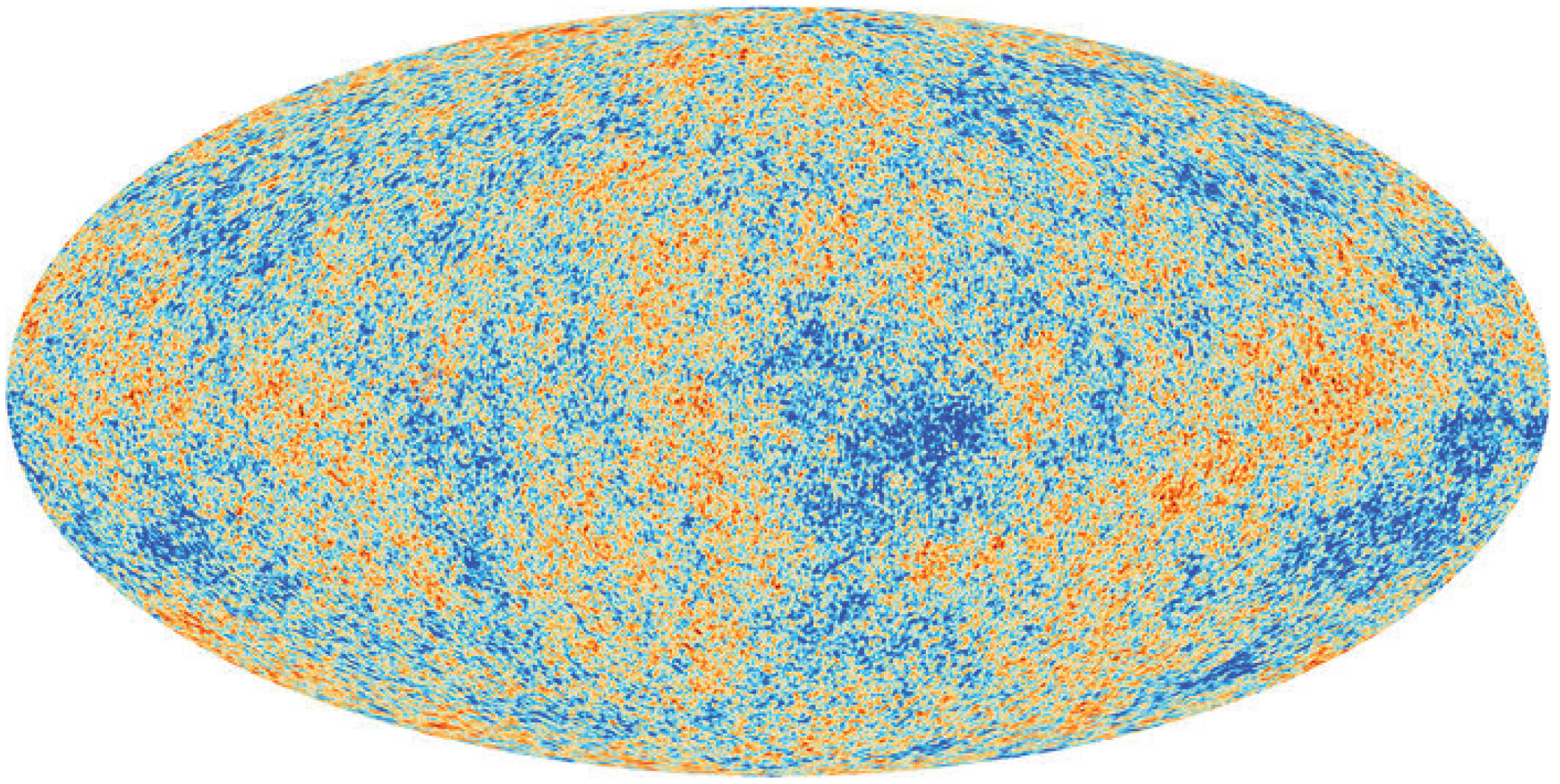
where $\theta$ and $\varphi$ defines a direction in the sky and $Y_{\ell m}$ are spherical harmonics, is an observable and has now been measured by many different experiments. The first one was the COBE satellite in 1992 [33]. The most recent and most accurate observation is by The European Space Agency (ESA) Planck satellite [17,18,19,20,21], see Figure 1. The so-called Sachs–Wolfe effect [34] relates the presence of small inhomogeneities, living in three-dimensional space and described by curvature perturbations $\zeta (\eta ,\mathit{x})$ to the temperature anisotropy of Figure 1, namely

$$\begin{array}{cc}\hfill \frac{\delta T}{T}\left(\mathit{e}\right)=& \int \frac{\mathrm{d}\mathit{k}}{{\left(2\pi \right)}^{3/2}}\left[F\left(\mathit{k}\right)+i\mathit{k}·\mathit{e}G\left(\mathit{k}\right)\right]{\zeta }_{\mathit{k}}\left({\eta }_{\mathrm{end}}\right)e^{-i\mathit{k}·\mathit{e}({\eta }_{\mathrm{lss}}-{\eta }_0)+i\mathit{k}·{\mathit{x}}_0},\hfill \end{array}$$

(4)

where $\mathit{e}$ is a unit vector in the direction of the observation on the celestial sphere defined by the angles $\theta$ and $\varphi$ and ${\zeta }_{\mathit{k}}\left(\eta \right)$ is the Fourier transform of $\zeta (\eta ,\mathit{x})$, namely $\zeta (\eta ,\mathit{x})={\left(2\pi \right)}^{-3/2}\int \mathrm{d}\mathit{k}{\zeta }_{\mathit{k}}\left(\eta \right)e^{i\mathit{k}·\mathit{x}}$. Notice that, because $\zeta (\eta ,\mathit{x})$ is real, one has ${\zeta }_{\mathit{k}}^{\ast }={\zeta }_{-\mathit{k}}$. The quantities ${\eta }_{\mathrm{lss}}$ and ${\eta }_0$ are the last scattering surface (lss) and present day (0) conformal times, respectively, while ${\mathit{x}}_0$ represents Earth’s location. The last scattering surface is the surface at which the CMB was emitted. It corresponds to the time at which our Universe became transparent and is located at a redshift of $z_{\mathrm{lss}}\simeq 1100$. The functions $F\left(\mathit{k}\right)$ and $G\left(\mathit{k}\right)$ are the so-called form factors and describe the evolution of the perturbation in the post-inflationary universe. They are not easy to calculate as they depend on the evolution of many different fluids in interaction. This evolution is usually tracked numerically [35]. However, it only depends on known physics and, therefore, can be subtracted away. Therefore, we see that temperature fluctuations are in fact directly given by ${\zeta }_{\mathit{k}}\left({\eta }_{\mathrm{end}}\right)$ evaluated at the end of inflation.

The behavior of curvature perturbations is controlled by the perturbed Einstein equations, $\delta G_{\mu \nu }=M_{\mathrm{Pl}}^{-2}\delta T_{\mu \nu }$. By definition, these equations are linear partial differential equations. However, they can be transformed into an infinite number of linear ordinary differential equations by going to Fourier space. One can then show [32] that curvature perturbation obeys

$$\begin{array}{c}\hfill {\left(z{\zeta }_{\mathit{k}}\right)}^{″}+\left(k^2-\frac{z^{″}}{z}\right)\left(z{\zeta }_{\mathit{k}}\right)=0,\end{array}$$

(5)

where we have defined $z\equiv a{M}_{\mathrm{Pl}}\sqrt{2{ϵ}_1}$. One recognizes the equation of motion of an oscillator whose fundamental frequency, ${\omega }^2=k^2-z^{″}/z$, is time-dependent. In other words, we deal with a parametric oscillator: a classical analogy would a pendulum the length of which can change in time. Here, the time dependence is fixed by z, which is only determined by the dynamics of the expansion since z depends on the scale factor and its derivatives. The solution to the above equations are easily analyzed. In an inflationary Universe, the Hubble radius $H^{-1}$ is constant while the wavelength of a given Fourier mode, which grows proportional to the scale factor, is stretched beyond the Hubble radius. Therefore, initially, $k^2\gg z^{″}/z$ (small scales limit) and the quantity $z{\zeta }_{\mathit{k}}$ oscillates

$$\begin{array}{c}\hfill z{\zeta }_{\mathit{k}}=A_{\mathit{k}}{e}^{ik\eta }+B_{\mathit{k}}{e}^{-ik\eta },\end{array}$$

(6)

where $A_{\mathit{k}}$ and $B_{\mathit{k}}$ are two arbitrary integration constants. The reason for this behavior is that the wavelength of the mode is so small that it does not feel the curvature of spacetime and behaves as if it lived in flat spacetime. In principle, the two constants $A_{\mathit{k}}$ and $B_{\mathit{k}}$ are fixed by the initial conditions. At the classical level, it is just unclear what these ones should be. Then, as time goes on, the mode exits the Hubble radius and the regime $k^2\ll z^{″}/z$ (large scales limit) becomes relevant. In that case, the solution can be written

$$\begin{array}{c}\hfill z{\zeta }_{\mathit{k}}=C_{\mathit{k}}z+D_{\mathit{k}}z{\int }^{\eta }\frac{\mathrm{d}\tau }{z^2\left(\tau \right)},\end{array}$$

(7)

where $C_{\mathit{k}}$ and $D_{\mathit{k}}$ are two constants of integrations. The first branch, proportional to $C_{\mathit{k}}$, is the growing mode and the second one the decaying mode. This can easily be verified if, for instance, one considers scale factors of the form $a\left(\eta \right)\propto {(-\eta )}^{1+\beta }$, recalling that inflation corresponds to $\beta \simeq -2$ and that the conformal time during inflation is negative and tends to zero (by negative values) as inflation proceeds. The above solution shows that the growing mode is, on large scales, constant, namely ${\zeta }_{\mathit{k}}\simeq C_{\mathit{k}}$, which means that the curvature perturbation has the advantage (among others) to be conserved on large scales.

Usually, the properties of CMB anisotropies are characterized by the correlation functions of $\delta T\left(\mathit{e}\right)/T$ which are, thanks to Equation (4), directly related to the correlation functions of curvature perturbation at the end of inflation. The two-point correlation function of $\zeta (\eta ,\mathit{x})$ reads

$$\begin{array}{cc}\hfill 〈\zeta (\eta ,\mathit{x})\zeta (\eta ,\mathit{x}+\mathit{r})〉& ={\int }_0^{+\infty }\frac{\mathrm{d}k}{k}\frac{sin\left(kr\right)}{kr}\frac{k^3}{2{\pi }^2}{\left|{\zeta }_{\mathit{k}}\left({\eta }_{\mathrm{end}}\right)\right|}^2,\hfill \end{array}$$

(8)

where the brackets are supposed to represent an average over some classical distribution such that $\langle {\zeta }_{\mathit{k}}{\zeta }_{\mathit{p}}^{\ast }\rangle ={\left|{\zeta }_{\mathit{k}}\right|}^2\delta (\mathit{k}-\mathit{p})$. At the end of inflation, ${\zeta }_{\mathit{k}}\left({\eta }_{\mathrm{end}}\right)\simeq C_{\mathit{k}}$ since, as explained before, the decaying mode can be neglected. However, one needs to specify the scale dependence of $C_{\mathit{k}}$. This can be done by matching the large scale regime to the small scale regime which, in practice, amounts to express $C_{\mathit{k}}$ in terms of $A_{\mathit{k}}$ and $B_{\mathit{k}}$. The problem is thus moved to determining the scale dependence of the coefficients $A_{\mathit{k}}$ and $B_{\mathit{k}}$. At the classical level, as mentioned before, there is just no clear approach of how this can be done in a well-justified and well-motivated way.

2.2. Quantum Perturbations

The above considerations, therefore, leave one important question unanswered: what is the origin of these perturbations? The beauty of inflation is that it can also provide an answer to this important question: inflation says that the primordial perturbations originate from the vacuum quantum fluctuations of the inflaton and gravitational fields at the beginning of inflation. This means that all structures in our Universe are nothing but quantum fluctuations stretched over cosmological distances by the expansion of the Universe and amplified by gravitational instability.

At the technical level, this means that, now, the perturbed metric $\delta g_{\mu \nu }$ is viewed as a quantum operator, $\delta {\widehat{g}}_{\mu \nu }$, satisfying the quantum perturbed Einstein equations, viewed as equations for quantum operators $\delta {\widehat{G}}_{\mu \nu }=M_{\mathrm{Pl}}^{-2}\delta {\widehat{T}}_{\mu \nu }$. Even more concretely, in this formulation, curvature perturbation can be viewed as a (test) quantum scalar field living in the expanding spacetime and can be written as

$$\begin{array}{c}\hfill z\left(\eta \right)\widehat{\zeta }(\eta ,\mathit{x})=\frac{1}{{\left(2\pi \right)}^{3/2}}\int \frac{\mathrm{d}\mathit{k}}{\sqrt{2k}}\left[{\widehat{c}}_{\mathit{k}}\left(\eta \right)e^{i\mathit{k}·\mathit{x}}+{\widehat{c}}_{\mathit{k}}^{†}\left(\eta \right)e^{-i\mathit{k}·\mathit{x}}\right],\end{array}$$

(9)

where ${\widehat{c}}_{\mathit{k}}\left(\eta \right)$ and ${\widehat{c}}_{\mathit{k}}^{†}\left(\eta \right)$ are the annihilation and creation operators satisfying the usual equal time commutation relations, $[{\widehat{c}}_{\mathit{k}}\left(\eta \right),{\widehat{c}}_{\mathit{p}}^{†}\left(\eta \right)]=\delta (\mathit{k}-\mathit{p})$. Curvature perturbations are then related to the creation and annihilation operators through

$$\begin{array}{c}\hfill z\left(\eta \right){\widehat{\zeta }}_{\mathit{k}}=\frac{1}{\sqrt{2k}}\left({\widehat{c}}_{\mathit{k}}+{\widehat{c}}_{-\mathit{k}}^{†}\right),z\left(\eta \right){\widehat{\zeta }}_{\mathit{k}}^{\prime }=-i\sqrt{\frac{k}{2}}\left({\widehat{c}}_{\mathit{k}}-{\widehat{c}}_{-\mathit{k}}^{†}\right).\end{array}$$

(10)

We notice that ${\widehat{\zeta }}_{\mathit{k}}$ and ${\widehat{\zeta }}_{\mathit{k}}^{\prime }$ mix creation and annihilation operators of momentum $\mathit{k}$ and $-\mathit{k}$.

The evolution of $\widehat{\zeta }(\eta ,\mathit{x})$ is controlled by the following Hamiltonian

$$\begin{array}{c}\hfill \widehat{H}={\int }_{{ℝ}^3}{\mathrm{d}}^3\mathit{k}\left[\frac{k}{2}\left({\widehat{c}}_{\mathit{k}}{\widehat{c}}_{\mathit{k}}^{†}+{\widehat{c}}_{-\mathit{k}}^{†}{\widehat{c}}_{-\mathit{k}}\right)-\frac{i}{2}\frac{z^{\prime }}{z}\left({\widehat{c}}_{\mathit{k}}{\widehat{c}}_{-\mathit{k}}-{\widehat{c}}_{-\mathit{k}}^{†}{c}_{\mathit{k}}^{†}\right)\right].\end{array}$$

(11)

This Hamiltonian comes from a second order expansion in $\zeta$ of the action of GR plus a scalar field (since inflation is driven by this type of field). This action (and, therefore, the corresponding Hamiltonian) remains quadratic in $\zeta$ and higher order terms are ignored because the perturbations are small. As already mentioned, this is well established at the time of recombination where the deviations are measured to be of the order ${10}^{-5}$. Since the fluctuations grow by gravitational instability, there were certainly even smaller during inflation.

The Hamiltonian (11) is made of two pieces. The first part describes the free Hamiltonian of a collection of harmonic oscillators with fundamental frequency $\omega =k$ (as appropriate for massless excitations). The second piece describes the interaction of the quantum field $\widehat{\zeta }(\eta ,\mathit{x})$ with the classical background characterized by the scale factor $a\left(\eta \right)$. If space-time is static (namely Minkowski space-time), then $a^{\prime }=0$ and the “time-dependent” coupling constant $z^{\prime }/z$ vanishes. This term is responsible for particle creation. Moreover, the momentum structure of this second piece in ${\widehat{c}}_{\mathit{k}}{\widehat{c}}_{-\mathit{k}}$ or ${\widehat{c}}_{-\mathit{k}}^{†}{c}_{\mathit{k}}^{†}$ indicates that particles are created by pairs with opposite momenta (in accordance with momentum conservation). At this point, one should clarify the following. In quantum field theory, quadratic action (or Hamiltonian) usually describes free fields while interactions are described as higher order terms. There is, however, one exception, namely the case where a quantum field interacts with a classical source. It is still described by a quadratic action, the presence of the interaction manifesting itself only by giving a time dependence to the effective frequency of the field oscillators. In other words, a free field is equivalent to a collection of harmonic oscillators while a field in interaction with a classical source is equivalent to a collection of parametric oscillators. The classic example is the Schwinger effect, where a fermionic field interacts with a classical electric field [16,36]. The case of a scalar field in a cosmological background is another example.

The Heisenberg equation, $i\mathrm{d}{\widehat{c}}_{\mathit{k}}/\mathrm{d}\eta =[{\widehat{c}}_{\mathit{k}},\widehat{H}]$, allows us to calculate the equation of motion of the operator ${\widehat{\zeta }}_{\mathit{k}}\left(\eta \right)$. This leads to

$$\begin{array}{c}\hfill \frac{\mathrm{d}{\widehat{c}}_{\mathit{k}}}{\mathrm{d}\eta }=-ik{\widehat{c}}_{\mathit{k}}+\frac{z^{\prime }}{z}{\widehat{c}}_{-\mathit{k}}^{†},\end{array}$$

(12)

from which one deduces that

$$\begin{array}{c}\hfill {\left(z{\widehat{\zeta }}_{\mathit{k}}\right)}^{″}+\left(k^2-\frac{z^{″}}{z}\right)\left(z{\widehat{\zeta }}_{\mathit{k}}\right)=0,\end{array}$$

(13)

that is to say, Equation (5) but written at the operator level.

A fundamental assumption of inflation is that the system starts in the vacuum state $|0\rangle$ defined by the condition ${\widehat{c}}_{\mathit{k}}\left({\eta }_{\mathrm{ini}}\right)|0\rangle =0$. In order to see what this implies for the field ${\widehat{\zeta }}_{\mathit{k}}\left(\eta \right)$, let us first solve the time dependence of the creation and annihilation operators—see Equation (12). This can be done by means of a Bogoliubov transformation, namely

$$\begin{array}{c}\hfill {\widehat{c}}_{\mathit{k}}\left(\eta \right)=u_k\left(\eta \right){\widehat{c}}_{\mathit{k}}({\eta }_{\mathrm{ini}})+v_k\left(\eta \right){\widehat{c}}_{-\mathit{k}}^{†}({\eta }_{\mathrm{ini}}),\end{array}$$

(14)

where the functions $u_k\left(\eta \right)$ and $v_k\left(\eta \right)$ obey

$$\begin{array}{cc}\hfill i\frac{\mathrm{d}{u}_k}{\mathrm{d}\eta }& =k{u}_k+i\frac{z^{\prime }}{z}{v}_k^{\ast },i\frac{\mathrm{d}{v}_k}{\mathrm{d}\eta }=k{v}_k+i\frac{z^{\prime }}{z}{u}_k^{\ast },\hfill \end{array}$$

(15)

and, by definition, have initial conditions $u_k({\eta }_{\mathrm{ini}})=1$ and $v_k({\eta }_{\mathrm{ini}})=0$. Let us notice that $u_k$ and $v_k$ depend on the modulus of the wavenumber $\mathit{k}$ only. The Bogoliubov transformation allows us to re-express the field expansion as

$$\begin{array}{c}\hfill z\left(\eta \right)\widehat{\zeta }(\eta ,\mathit{x})=\frac{1}{{\left(2\pi \right)}^{3/2}}\int \frac{\mathrm{d}\mathit{k}}{\sqrt{2k}}\left[\left(u_k+v_k^{\ast }\right){\widehat{c}}_{\mathit{k}}({\eta }_{\mathrm{ini}})e^{i\mathit{k}·\mathit{x}}+\left(u_k^{\ast }+v_k\right){\widehat{c}}_{\mathit{k}}^{†}({\eta }_{\mathrm{ini}})e^{-i\mathit{k}·\mathit{x}}\right].\end{array}$$

(16)

It is easy to verify from Equation (15) that the function $u_k+v_k^{\ast }$ obeys the equation ${(u_k+v_k^{\ast })}^{″}+(k^2-z^{″}/z)(u_k+v_k^{\ast })=0$, namely the same equation as $z{\zeta }_{\mathit{k}}$. Recalling the initial conditions for $u_k$ and $v_k$, this implies that the mode function in (16), $(u_k+v_k^{\ast })/\sqrt{2k}$, behaves as

$$\begin{array}{c}\hfill \underset{k\eta \to -\infty }{lim}\frac{u_k+v_k^{\ast }}{\sqrt{2k}}=\frac{1}{\sqrt{2k}}{e}^{ik(\eta -{\eta }_{\mathrm{ini}})},\end{array}$$

(17)

in the small scales limit. In other words, the assumption that the fluctuations are quantum and start in the vacuum state has completely fixed the initial conditions. As a consequence, in Equation (6), one should choose

$$\begin{array}{c}\hfill A_{\mathit{k}}=\frac{1}{\sqrt{2k}}{e}^{-ik{\eta }_{\mathrm{ini}}},B_{\mathit{k}}=0.\end{array}$$

(18)

Then, the initial conditions being now known, the calculation of the power spectrum can be performed explicitly. Indeed, we no longer face the issues discussed after Equation (8): $C_{\mathit{k}}$ can be related to $A_{\mathit{k}}$ and $B_{\mathit{k}}$ but, as just explained, these ones are now fully determined. The calculation leads to an almost scale invariant power spectrum, ${\mathcal{P}}_{\zeta }\left(k\right)=k^3{\left|{\zeta }_{\mathit{k}}\left({\eta }_{\mathrm{end}}\right)\right|}^2/\left(2{\pi }^2\right)\simeq A_{\mathrm{S}}{k}^{n_{\mathrm{S}}-1}$, where $n_{\mathrm{S}}\simeq 1$ plus small corrections that depend on the model of inflation considered. Scale invariance means that, if $n_{\mathrm{S}}=1$, then ${\mathcal{P}}_{\zeta }\left(k\right)$ no longer depends on k. Since, according to inflation, $n_{\mathrm{S}}\simeq 1$ but $n_{\mathrm{S}}\ne 1$, we have in fact almost scale invariance. Moreover, measuring the small deviations from scale invariance allows us to constrain inflation since the corrections, as just mentioned above, depend on the scenario of inflation. The fact that $n_{\mathrm{S}}\simeq 1$ crucially rests on the choice $A_{\mathit{k}}\propto 1/\sqrt{2k}$. Had we have another scale dependence initially for $A_{\mathit{k}}$ and $B_{\mathit{k}}$, the power spectrum would have been completely different and, generically, far from scale invariance. Remarkably, according to the most recent data obtained by the Planck satellite [20,21], everything is precisely consistent with a power spectrum of the form ${\mathcal{P}}_{\zeta }\left(k\right)=A_{\mathrm{S}}{k}^{n_{\mathrm{S}}-1}$, with $ln\left({10}^{10}{A}_{\mathrm{S}}\right)=3.044\pm 0.014$ and $n_{\mathrm{S}}=0.9649\pm 0.0042$. The value of the spectral index $n_{\mathrm{S}}$ is not predicted by inflation (more precisely, if a model of inflation is given, then it is predicted. However, the problem is that the correct model of inflation is not known). It was known for a long time that $n_{\mathrm{S}}$ should be around one, but it is only very recently that Planck demonstrated that $n_{\mathrm{S}}\ne 1$ at a significant statistical level (namely more that $5\sigma$).

The Planck results are, therefore, one of the main reasons to trust inflation and its mechanism of structures formation according to which structures in the Universe are nothing but quantum fluctuations. This fascinating conclusion is now well supported by astrophysical data.

2.3. The Quantum State of Inflationary Perturbations

Before discussing the properties of the state of cosmological perturbations, let us make the following remark. We saw in Equation (10) that the definition of ${\widehat{\zeta }}_{\mathit{k}}$ mixes creation and annihilation operators of mode $\mathit{k}$ and $-\mathit{k}$. This is because, as already mentioned, particles are created by pair with opposite momenta. However, this is uncommon from a quantum information point of view where one likes to view the total system as a collection of subsystems associated with the different modes. In other words, if $\mathcal{E}$ is the Hilbert space of the full system and ${\mathcal{E}}_{\mathit{k}}$ the Hilbert space associated with the mode $\mathit{k}$, we would like to have $\mathcal{E}={\otimes }_{\mathit{k}}{\mathcal{E}}_{\mathit{k}}$. For this reason, we now introduce, for a fixed mode $\mathit{k}$, the “position” ${\widehat{q}}_{\mathit{k}}$ and the “momentum” ${\widehat{\pi }}_{\mathit{k}}$ defined by

$$\begin{array}{c}\hfill {\widehat{q}}_{\mathit{k}}=\frac{1}{\sqrt{2k}}\left({\widehat{c}}_{\mathit{k}}+{\widehat{c}}_{\mathit{k}}^{†}\right),{\widehat{\pi }}_{\mathit{k}}=-i\sqrt{\frac{k}{2}}\left({\widehat{c}}_{\mathit{k}}-{\widehat{c}}_{\mathit{k}}^{†}\right).\end{array}$$

(19)

These two operators are Hermitian. The relation between ${\widehat{\zeta }}_{\mathit{k}}$ and the position and momentum operators can be easily derived and reads

$$\begin{array}{c}\hfill z\left(\eta \right){\widehat{\zeta }}_{\mathit{k}}=\frac{1}{2}\left[{\widehat{q}}_{\mathit{k}}+{\widehat{q}}_{-\mathit{k}}+\frac{i}{k}\left({\widehat{\pi }}_{\mathit{k}}-{\widehat{\pi }}_{-\mathit{k}}\right)\right],z\left(\eta \right){\widehat{\zeta }}_{\mathit{k}}^{\prime }=\frac{1}{2i}\left[k\left({\widehat{q}}_{\mathit{k}}-{\widehat{q}}_{-\mathit{k}}\right)+i\left({\widehat{\pi }}_{\mathit{k}}+{\widehat{\pi }}_{-\mathit{k}}\right)\right].\end{array}$$

(20)

In the following, we consider a description of the system based on these operators since we want to make use of the formalism of quantum information. In fact, the above definitions allow us to describe cosmological perturbations as a continuous variable system. A continuous variable system is a system that is described by Hermitian operators satisfying canonical commutation relation, $[{\widehat{q}}_{\mathit{k}},{\widehat{\pi }}_{{\mathit{k}}^{\prime }}]=i\delta ({\mathit{k}}^{\prime }-\mathit{k})$. The number of degrees of freedom is infinite and labeled by the wavenumber $\mathit{k}$.

Another idea from Quantum Information Theory that will be playing an important role in the following is that of bipartite system. Indeed, for higher than a one-dimensional system, the set of degrees of freedom can be split into two subsets. This defines a partition and allows us to see the whole system as a bipartite system. Then, one can study the nature of the correlations between the two subsystems, which is a way to assess the “quantumness” of the whole system. An important point is that one can define several partitions for the same system. As an introductory example, let us consider a four-dimensional system with degrees of freedom ${\widehat{q}}_i$ and vector $\widehat{r}={({\widehat{q}}_i,{\widehat{\pi }}_i)}^{\mathrm{T}}$, $i=1,\cdots ,4$. We split the system into two subsystems, A and B, and defines a partition such that $\mathcal{E}={\mathcal{E}}_A\otimes {\mathcal{E}}_B$. For instance, we can choose the subsystem A to contain ${\widehat{q}}_1$ and ${\widehat{q}}_2$ and, therefore, to be described by ${\widehat{r}}_A={({\widehat{q}}_1,{\widehat{q}}_2,{\widehat{\pi }}_1,{\widehat{\pi }}_2)}^{\mathrm{T}}$ while the system B contains ${\widehat{q}}_3$ and ${\widehat{q}}_4$ and is described by ${\widehat{r}}_B={({\widehat{q}}_3,{\widehat{q}}_4,{\widehat{\pi }}_3,{\widehat{\pi }}_4)}^{\mathrm{T}}$. Then, we define the vector $\widehat{R}$ by $\widehat{R}={({\widehat{r}}_A,{\widehat{r}}_B)}^{\mathrm{T}}$. This definition of $\widehat{R}$, namely the way we list its components, is, implicitly, a definition of a partition. In Cosmology, because of pair creations, the partition $\mathcal{E}={\otimes }_{\mathit{k}\in {ℝ}^{3+}}{\mathcal{E}}_{\mathit{k}}\otimes {\mathcal{E}}_{-\mathit{k}}$ is, at least at first sight, very natural and, in the following, we work with it.

After these preliminary remarks, let us come back to the quantum state of the perturbations. As mentioned earlier, in Cosmology, one starts from the vacuum state ${\otimes }_{\mathit{k}}|0_{\mathit{k}},0_{-\mathit{k}}\rangle$ at time $\eta ={\eta }_{\mathrm{ini}}$; that is to say, ${\widehat{c}}_{\mathit{k}}\left({\eta }_{\mathrm{ini}}\right)|0\rangle =0$ and ${\widehat{c}}_{-\mathit{k}}\left({\eta }_{\mathrm{ini}}\right)|0\rangle =0$. Then, by solving the Schrödinger equation, with the Hamiltonian given by Equation (11), one can show that this state evolves into a two-mode squeezed state given by

$$\begin{array}{c}\hfill |{\Psi }_{2\mathrm{sq}}\rangle =\underset{\mathit{k}}{⨂}\frac{1}{cosh{r}_k}{\displaystyle \sum _{n=0}^{\infty }}{e}^{-2in{\phi }_k}{tanh}^n{r}_k|n_{\mathit{k}},n_{-\mathit{k}}\rangle ,\end{array}$$

(21)

where $|n_{\mathit{k}}\rangle$ is an eigenvector of the particle number operator in the mode $\mathit{k}$. $r_k$ and ${\phi }_k$ are the squeezing parameter and squeezing angle, respectively. They are time dependent functions controlled by the following equations:

$$\begin{array}{c}\hfill \frac{\mathrm{d}{r}_k}{\mathrm{d}\eta }=\frac{z^{\prime }}{z}cos\left(2{\phi }_k\right),\frac{\mathrm{d}{\phi }_k}{\mathrm{d}\eta }=-k-\frac{z^{\prime }}{z}coth\left(2r_k\right)sin\left(2{\phi }_k\right).\end{array}$$

(22)

The fact that we encounter a squeezed state should not come as a surprise. It is indeed well known that, while the quantization of an harmonic oscillator naturally leads to coherent states, the quantization of a parametric oscillator leads to squeezed states. Since we saw before that, because of its interaction with the dynamical scale factor, the field ${\widehat{\zeta }}_{\mathit{k}}$ acquires a time-dependent fundamental frequency, and, therefore, can be viewed as parametric oscillator, the whole picture appears to be consistent.

2.4. Physical Interpretation

Let us now come back to the quantum state (21) and try to gain physical intuition about it. The corresponding wavefunction can be expressed as

$$\begin{array}{c}\hfill {\Psi }_{2\mathrm{sq}}\left(q_{\mathit{k}},q_{-\mathit{k}}\right)=〈q_{\mathit{k}},q_{-\mathit{k}}\left|\frac{1}{cosh{r}_k}{\displaystyle \sum _{n=0}^{\infty }}{e}^{-2in{\phi }_k}{tanh}^n{r}_k\right|n_{\mathit{k}},n_{-\mathit{k}}〉=\frac{e^{A(r_k,{\phi }_k)(q_{\mathit{k}}^2+q_{-\mathit{k}}^2)-B(r_k,{\phi }_k)q_{\mathit{k}}{q}_{-\mathit{k}}}}{cosh{r}_k\sqrt{\pi }\sqrt{1-e^{-4i{\phi }_k}{tanh}^2{r}_k}},\end{array}$$

(23)

where the functions $A(r_k,{\phi }_k)$ and $B(r_k,{\phi }_k)$ are given by

$$\begin{array}{c}\hfill A(r_k,{\phi }_k)=\frac{e^{-4i{\phi }_k}{tanh}^2{r}_k+1}{2(e^{-4i{\phi }_k}{tanh}^2{r}_k-1)},B(r_k,{\phi }_k)=\frac{2e^{-2i{\phi }_k}tanh{r}_k}{e^{-4i{\phi }_k}{tanh}^2{r}_k-1}.\end{array}$$

(24)

This explicit form for the wave function allows us to understand what, physically, a two-mode squeezed state means [37]. Before treating the case of a two-mode squeezed state, however, let us recall some well-known facts. Let us consider one mode $\mathit{k}$. The corresponding vacuum state is a coherent state, that is to say, a state with wavefunction in position space given by

$${\Psi }_0\left(q_{\mathit{k}}\right)=\frac{1}{{\pi }^{1/4}}{e}^{-{\left(q_{\mathit{k}}\right)}^2/2},$$

(25)

which is nothing but the wavefunction for the ground state of the harmonic oscillator in non-relativistic quantum mechanics. The same state, written in momentum basis, can be expressed as ${\tilde{\Psi }}_0\left({\pi }_{\mathit{k}}\right)=\frac{1}{{\pi }^{1/4}}{e}^{-{\left({\pi }_{\mathit{k}}\right)}^2/2}$. From the knowledge of the wave function, one can calculate the dispersion in field amplitude and momentum. This gives $\langle \Delta {\widehat{q}}_{\mathit{k}}^2\rangle =\langle \Delta {\widehat{\pi }}_{\mathit{k}}^2\rangle =1/2$, which saturates the Heisenberg inequality, namely $\langle \Delta {\widehat{q}}_{\mathit{k}}^2\rangle \langle \Delta {\widehat{\pi }}_{\mathit{k}}^2\rangle =1/4$.

Let us now consider a one-mode squeezed state. Its wave function, in field amplitude and conjugate momentum basis, can be written as

$${\Psi }_R\left(q_{\mathit{k}}\right)=\frac{\sqrt{R}}{{\pi }^{1/4}}{e}^{-R^2{\left(q_{\mathit{k}}\right)}^2/2},{\tilde{\Psi }}_R\left({\pi }_{\mathit{k}}\right)=\frac{1}{{\pi }^{1/4}\sqrt{R}}{e}^{-{\left({\pi }_{\mathit{k}}\right)}^2/\left(2R^2\right)},$$

(26)

where we have introduced a new parameter, R. The physical interpretation of this parameter can be found by calculating again the dispersion in position and momentum. One finds $\langle \Delta {\widehat{q}}_{\mathit{k}}^2\rangle =1/\left(2R^2\right)$ and $\langle \Delta {\widehat{\pi }}_{\mathit{k}}^2\rangle =R^2/2$. Although they still saturate the Heisenberg inequality, the two dispersions are no longer equal. If $R>1$, then the dispersion in field amplitude is smaller than the dispersion in conjugate momentum (and, interestingly enough, smaller than that of the vacuum state). We say that the state is squeezed in position or field amplitude, hence its name. Of course, since one has to satisfy the Heisenberg inequality, the dispersion in momentum is larger. If $R<1$, we have the opposite situation and the state is squeezed in momentum.

After these preliminary comments, we now come to the two-mode squeezed state. As the name of the state indicates, we must now consider two modes and, of course, we choose $\mathit{k}$ and $-\mathit{k}$. Following the tradition in quantum information theory, we can also call mode $\mathit{k}$ “Alice” and mode $-\mathit{k}$ “Bob”. In field amplitude basis, the vacuum state of this bipartite system can be written as

$${\Psi }_0\left(q_{\mathit{k}},q_{-\mathit{k}}\right)=\frac{1}{\sqrt{\pi }}{e}^{-{\left(q_{\mathit{k}}\right)}^2/2-{\left(q_{-\mathit{k}}\right)}^2/2}=\frac{1}{\sqrt{\pi }}{e}^{-{(q_{\mathit{k}}-q_{-\mathit{k}})}^2/4}{e}^{-{(q_{\mathit{k}}+q_{-\mathit{k}})}^2/4}.$$

(27)

We see that the position of Alice and Bob are uncorrelated. Then, in a way which is exactly similar to what has already been done above, we introduce the following state:

$${\Psi }_R\left(q_{\mathit{k}},q_{-\mathit{k}}\right)=\frac{1}{\sqrt{\pi }}{e}^{-R^2{(q_{\mathit{k}}-q_{-\mathit{k}})}^2/4}{e}^{-{(q_{\mathit{k}}+q_{-\mathit{k}})}^2/\left(4R^2\right)}=\frac{1}{\sqrt{\pi }}{e}^{\overline{A}\left(R\right)(q_{\mathit{k}}^2+q_{-\mathit{k}}^2)-\overline{B}\left(R\right)q_{\mathit{k}}{q}_{-\mathit{k}}},$$

(28)

where the squeezing factor R appears again and where the two functions $\overline{A}\left(R\right)$ and $\overline{B}\left(R\right)$ are defined by

$$\begin{array}{c}\hfill \overline{A}\left(R\right)\equiv -\frac{1}{4}\left(R^2+\frac{1}{R^2}\right),\overline{B}\left(R\right)\equiv -\frac{1}{2}\left(R^2-\frac{1}{R^2}\right).\end{array}$$

(29)

The state (28) is, by definition, a two-mode squeezed state. Clearly, since Equations (23) and (28) are similar, this means that the state (23) is also a two-mode squeezed state. In Equation (28), we have ignored the squeezed angle and, therefore, we should identify the function $\overline{A}\left(R\right)$ with $A(r_k,0)=-(e^{2r_k}+e^{-2r_k})/4$, which immediately leads to $r_k=lnR$. One checks that this is consistent since $B(r_k,0)=-(e^{2r_k}-e^{-2r_k})/2$ is indeed equal to $\overline{B}\left(R\right)$ and the normalization factor $cosh{r}_k\sqrt{1-e^{-4i{\phi }_k}{tanh}^2{r}_k}$ goes to one when the squeezing angle is zero. We notice that the positions of Alice and Bob are now correlated and that these correlations are genuinely quantum since the state (28) is an entangled state, namely ${\Psi }_R\left(q_{\mathit{k}},q_{-\mathit{k}}\right)\ne {\Psi }_R\left(q_{\mathit{k}}\right){\Psi }_R\left(q_{-\mathit{k}}\right)$. This means that the state (23) implies the existence of genuine quantum correlations between the field amplitudes $q_{\mathit{k}}$ and $q_{-\mathit{k}}$. It is also interesting to remark that the two-mode squeezed state does not lead to squeezing for Alice or Bob. Indeed, it is easy to verify that $\langle \Delta {\widehat{q}}_{\mathit{k}}^2\rangle =\langle \Delta {\widehat{q}}_{-\mathit{k}}^2\rangle =(1+R^4)/\left(4R^2\right)$. These dispersions are always larger than the dispersions obtained for the vacuum state. This is related to the fact that, if one traces out, say, Alice’s degree of freedom, one is left with a state for Bob that is not a one-mode squeezed state but a thermal state.

The two-mode squeezed state that is present in Cosmology is quite peculiar: it is probably the strongest squeezed state ever produced in Nature. The squeezing factor is often expressed in decibel with the help of the following definition—see also Equations (14) and (15) of Ref. [38]

$$\begin{array}{c}\hfill -10{log}_{10}\left(e^{-2r}\right)\mathrm{dB}=\frac{20r}{ln10}\mathrm{dB}.\end{array}$$

(30)

In Cosmology, one can achieve $r\simeq 50$, which means a squeezing of ≃43 dB to be compared with ~15 dB, which is the world record in the lab—see Refs. [39,40].

2.5. Gaussian States

Another interesting property of a two mode squeezed state is that it belongs to a wider class of quantum states called “Gaussian states”. We indeed check that the wavefunction (23) is Gaussian. Gaussian states play a fundamental role in quantum mechanics. They arise in many different branches of Physics such as Laser Physics, Quantum Field Theory (in curved spacetime or not), Solid State Physics or Cosmology and they are ubiquitous in Quantum Information Theory. Gaussian states naturally occur as ground (coherent or squeezed) or thermal equilibrium states of any physical quantum system described by a quadratic Hamiltonian. Moreover, with existing technologies, they are easily manipulable in the lab.

At the technical level, a Gaussian state is a state the characteristic function of which is a Gaussian. The characteristic function $\chi \left(\xi \right)$ is defined by

$$\begin{array}{c}\hfill \chi \left(\xi \right)=\mathrm{Tr}\left[\widehat{\rho }\widehat{\mathcal{W}}\left(\xi \right)\right],\end{array}$$

(31)

where $\widehat{\rho }$ is the density matrix of the quantum state and where $\widehat{\mathcal{W}}\left(\xi \right)$ is the Weyl operator which can be expressed as

$$\begin{array}{c}\hfill \widehat{\mathcal{W}}\left(\xi \right)=e^{i{\xi }^{\mathrm{T}}\widehat{R}},\end{array}$$

(32)

where the vector $\widehat{R}$ has already been introduced before and is defined by $\widehat{R}={(k^{1/2}{\widehat{q}}_{\mathit{k}},k^{-1/2}{\widehat{\pi }}_{\mathit{k}},k^{1/2}{q}_{-\mathit{k}},k^{-1/2}{\widehat{\pi }}_{-\mathit{k}})}^{\mathrm{T}}$ (here, we have slightly modified the definition by introducing a $k^{1/2}$ in front of positions and a $k^{-1/2}$ in front of momentum in order to work with dimensionless quantities). For a two-mode squeezed state, the characteristic function is indeed a Gaussian (justifying the fact that it belongs to the class of Gaussian states)

$$\begin{array}{c}\hfill \chi ({\xi }_1,{\xi }_2,{\xi }_3,{\xi }_4)=e^{-{\xi }^{\mathrm{T}}\gamma \xi /4},\end{array}$$

(33)

where $\gamma$ is the covariance matrix is given

$$\begin{array}{c}\hfill \gamma =\left(\begin{array}{cccc}cosh\left(2r_k\right)& 0& sinh\left(2r_k\right)cos\left(2{\phi }_k\right)& sinh\left(2r_k\right)sin\left(2{\phi }_k\right)\\ 0& cosh\left(2r_k\right)& sinh\left(2r_k\right)sin\left(2{\phi }_k\right)& -sinh\left(2r_k\right)cos\left(2{\phi }_k\right)\\ sinh\left(2r_k\right)cos\left(2{\phi }_k\right)& sinh\left(2r_k\right)sin\left(2{\phi }_k\right)& cosh\left(2r_k\right)& 0\\ sinh\left(2r_k\right)sin\left(2{\phi }_k\right)& -sinh\left(2r_k\right)cos\left(2{\phi }_k\right)& 0& cosh\left(2r_k\right)\end{array}\right).\end{array}$$

(34)

The covariance matrix is related to the two point correlation function of the position and/or momentum operators since $\langle {\widehat{R}}_i{\widehat{R}}_j\rangle ={\gamma }_{ij}/2+i{J}_{ij}/2$ where the matrix J is defined by

$$\begin{array}{c}\hfill J=\left(\begin{array}{cccc}0& 1& 0& 0\\ -1& 0& 0& 0\\ 0& 0& 0& 1\\ 0& 0& -1& 0\end{array}\right).\end{array}$$

(35)

Another, equivalent, way to define a Gaussian state is the following: a Gaussian state is a state which has a Gaussian Wigner function. For a state with density matrix $\widehat{\rho }$, the Wigner function is defined by

$$\begin{array}{c}\hfill W\left(R\right)=\frac{1}{{\left(2\pi \right)}^2}\int \mathrm{d}x\mathrm{d}y{e}^{-i{\pi }_{\mathit{k}}x-i{\pi }_{-\mathit{k}}y}〈q_{\mathit{k}}+\frac{x}{2},q_{-\mathit{k}}+\frac{y}{2}\left|\widehat{\rho }\right|q_{\mathit{k}}-\frac{x}{2},q_{-\mathit{k}}-\frac{y}{2}〉.\end{array}$$

(36)

Physically, the Wigner function is the quantum generalization of the classical distribution in phase space. It is related to the characteristic function introduced before by the formula

$$\begin{array}{c}\hfill W\left(\xi \right)=\frac{1}{{\left(2\pi \right)}^4}\int {\mathrm{d}}^4\eta e^{-i{\xi }^{\mathrm{T}}\eta }\chi \left(\eta \right).\end{array}$$

(37)

Using this result and the characteristic function of a Gaussian state, see Equation (33), it is easy to demonstrate that

$$\begin{array}{c}\hfill W\left(\xi \right)=\frac{1}{{\pi }^2\sqrt{det\gamma }}{e}^{-{\xi }^{\mathrm{T}}{\gamma }^{-1}\xi }.\end{array}$$

(38)

This shows that the Wigner function is also a Gaussian. If one uses the expression (34) of the covariance matrix, then the explicit expression of the Wigner function of a two-mode squeezed state reads

$$\begin{array}{cc}\hfill W& =\frac{1}{{\pi }^2}exp[-\left(k{q}_{\mathit{k}}^2+k{q}_{-\mathit{k}}^2+\frac{{\pi }_{\mathit{k}}^2}{k}+\frac{{\pi }_{-\mathit{k}}^2}{k}\right)cosh\left(2r_k\right)+2\left(q_{\mathit{k}}{\pi }_{\mathit{k}}+q_{-\mathit{k}}{\pi }_{-\mathit{k}}\right)sin\left(2{\phi }_k\right)sinh\left(2r_k\right)\hfill \\ & +2\left(k{q}_{\mathit{k}}{q}_{-\mathit{k}}-\frac{{\pi }_{\mathit{k}}{\pi }_{-\mathit{k}}}{k}\right)cos\left(2{\phi }_k\right)sinh\left(2r_k\right)].\hfill \end{array}$$

(39)

3. The Quantum-to-Classical Transition of the Cosmological Perturbations

From the above considerations, why curvature perturbations are viewed as genuinely quantum should now be clear. However, when CMB anisotropies are analyzed by astronomers, curvature perturbations are treated classically without any reference to their quantum origin. Is this just wrong or can we justify this approach by claiming that some sort of quantum-to-classical transition took place in the early Universe? This question is reminiscent of the question of classical limit in Quantum Mechanics. It is known that this problem is subtle and we will argue that, in the context of Cosmology, it is even more subtle than in ordinary situations.

3.1. Stochastic Description?

The fact that a two-mode squeezed state is Gaussian implies, as discussed before, that its Wigner function is positive definite. In fact, one can show that the only states for which this is the case are precisely the Gaussian states [41]. This leads to the idea that the Wigner function could be used as a classical distribution over phase space. If so, this would mean that there exists a classical, stochastic, description of the properties of the system. This would indicate that a quantum-to-classical transition has taken place. At the technical level, the previous argument can be formulated as follows. Let us consider a function O of position and momentum, namely $O(q_{\mathit{k}},{\pi }_{\mathit{k}},q_{-\mathit{k}},{\pi }_{-\mathit{k}})$. According to the above considerations, one would define the classical average of O as

$$\begin{array}{c}\hfill {\langle O\rangle }_{\mathrm{stocha}}=\int O\left(R\right)W\left(R\right){\mathrm{d}}^{4}R.\end{array}$$

(40)

Using the correspondence principle, one can define the corresponding operator $\widehat{O}$ as $\widehat{O}=O({\widehat{q}}_{\mathit{k}},{\widehat{\pi }}_{\mathit{k}},{\widehat{q}}_{-\mathit{k}},{\widehat{\pi }}_{-\mathit{k}})$. If the system is classical, then one must have

$$\begin{array}{c}\hfill \langle \widehat{O}\rangle ={〈O〉}_{\mathrm{stocha}}.\end{array}$$

(41)

We now establish under which conditions the above equation holds. Let us first define the Weyl transform of the operator $\widehat{O}$ by

$$\begin{array}{c}\hfill \tilde{O}(q_{\mathit{k}},{\pi }_{\mathit{k}},q_{-\mathit{k}},{\pi }_{-\mathit{k}})=\int \mathrm{d}x\mathrm{d}y{e}^{-i{\pi }_{\mathit{k}}x-i{\pi }_{-\mathit{k}}y}〈q_{\mathit{k}}+\frac{x}{2},q_{-\mathit{k}}+\frac{y}{2}\left|\widehat{O}\right|q_{\mathit{k}}-\frac{x}{2},q_{-\mathit{k}}-\frac{y}{2}〉.\end{array}$$

(42)

It is of course reminiscent of the Wigner function. In fact, up to a factor ${\left(2\pi \right)}^{-2}$, the Wigner function is the Weyl transform of the density matrix, namely $\tilde{\rho }={\left(2\pi \right)}^{2}W$. The Weyl transform associates a function in phase space with any operator in Hilbert space. The fundamental property of the Weyl transform is that, for two operators $\widehat{A}$ and $\widehat{B}$, one has

$$\begin{array}{c}\hfill \mathrm{Tr}\left(\widehat{A}\widehat{B}\right)=\frac{1}{{\left(2\pi \right)}^2}\int \tilde{A}\left(R\right)\tilde{B}\left(R\right){\mathrm{d}}^{4}R,\end{array}$$

(43)

where the seemingly awkward factor ${\left(2\pi \right)}^2$ comes from the fact that the subspace we consider here is four-dimensional. It follows that

$$\begin{array}{c}\hfill \langle \widehat{O}\rangle =\mathrm{Tr}(\widehat{\rho }\widehat{O})=\frac{1}{{\left(2\pi \right)}^2}\int \tilde{\rho }\left(R\right)\tilde{O}\left(R\right){\mathrm{d}}^{4}R=\int \tilde{O}\left(R\right)W\left(R\right){\mathrm{d}}^{4}R.\end{array}$$

(44)

Comparing the above formula to Equation (40), we see that quantum and stochastic averages coincide if

$$\begin{array}{c}\hfill O\left(R\right)=\tilde{O}\left(R\right).\end{array}$$

(45)

Therefore, whether or not a quantum-to-classical transition takes place can be summarized in the above equation and to whether it holds in general. For instance, it is easy to show that it is always valid for any power of the operator ${\widehat{q}}_{\mathit{k}}^m$, namely $\widetilde{q_{\mathit{k}}^m}=q_{\mathit{k}}^m$. In the same fashion, one also has $\widetilde{{\pi }_{\mathit{k}}^m}={\pi }_{\mathit{k}}^m$. However, $\widetilde{q_{\mathit{k}}{\pi }_{\mathit{k}}}=q_{\mathit{k}}{\pi }_{\mathit{k}}+i/2$. For quadratic combinations, one can summarize the previous results as

$$\begin{array}{c}\hfill \widetilde{R_j{R}_k}=R_j{R}_k+\frac{1}{2}\left[{\widehat{R}}_j,{\widehat{R}}_k\right]=R_j{R}_k+\frac{i}{2}{J}_{jk},\end{array}$$

(46)

where the matrix J has been defined in Equation (35). Moreover, any combination of operators of mode $\mathit{k}$ and mode $-\mathit{k}$ has a trivial Weyl transform, for instance $\widetilde{q_{\mathit{k}}^{m_1}{\pi }_{-\mathit{k}}^{m_2}}=q_{\mathit{k}}^{m_1}{\pi }_{-\mathit{k}}^{m_2}$. Using Equation (20), one can now calculate $\widetilde{{\zeta }_{\mathit{k}}^2}$ in order to see whether a stochastic calculation of the curvature perturbations power spectrum is possible. The previous results imply that

$$\begin{array}{cc}\hfill z^2\left(\eta \right)\widetilde{{\zeta }_{\mathit{k}}^2}& =\frac{1}{4}[\widetilde{q_{\mathit{k}}^2}+\widetilde{q_{-\mathit{k}}^2}+\widetilde{q_{\mathit{k}}{q}_{-\mathit{k}}}+\widetilde{q_{-\mathit{k}}{q}_{\mathit{k}}}+\frac{i}{k}\left(\widetilde{q_{\mathit{k}}{\pi }_{\mathit{k}}}+\widetilde{{\pi }_{\mathit{k}}{q}_{\mathit{k}}}\right)-\frac{i}{k}\left(\widetilde{q_{-\mathit{k}}{\pi }_{-\mathit{k}}}+\widetilde{{\pi }_{-\mathit{k}}{q}_{-\mathit{k}}}\right)\hfill \\ & +\frac{i}{k}\left(\widetilde{q_{-\mathit{k}}{\pi }_{\mathit{k}}}-\widetilde{q_{\mathit{k}}{\pi }_{-\mathit{k}}}+\widetilde{{\pi }_{\mathit{k}}{q}_{-\mathit{k}}}-\widetilde{{\pi }_{-\mathit{k}}{q}_{\mathit{k}}}\right)-\frac{1}{k^2}\left(\widetilde{{\pi }_{\mathit{k}}^2}+\widetilde{{\pi }_{-\mathit{k}}^2}-\widetilde{{\pi }_{\mathit{k}}{\pi }_{-\mathit{k}}}-\widetilde{{\pi }_{-\mathit{k}}{\pi }_{\mathit{k}}}\right)].\hfill \end{array}$$

(47)

Among all the terms in the above expression, only the last four on the first line have a non-trivial Weyl transform. However, if $\widetilde{q_{\mathit{k}}{\pi }_{\mathit{k}}}$ and $\widetilde{{\pi }_{\mathit{k}}{q}_{\mathit{k}}}$ have, separately, a non-trivial Weyl transform, the sum of these two terms actually has a trivial Weyl transform because the additional factor $i/2$ originating from Equation (46) cancel out. Therefore, we conclude that $\widetilde{{\zeta }_{\mathit{k}}^2}={\zeta }_{\mathit{k}}^2$. As a consequence, the quantum two-point correlation function of curvature perturbations, $\langle \widehat{\zeta }(\eta ,\mathit{x})\widehat{\zeta }(\eta ,\mathit{y})\rangle$ can be exactly reproduced in a classical, stochastic, approach. One can also show that this is the case for $\langle \widehat{\zeta }(\eta ,\mathit{x}){\widehat{\zeta }}^{\prime }(\eta ,\mathit{y})+{\widehat{\zeta }}^{\prime }(\eta ,\mathit{x})\widehat{\zeta }(\eta ,\mathit{y})\rangle$ or $\langle {\widehat{\zeta }}^{\prime }(\eta ,\mathit{x}){\widehat{\zeta }}^{\prime }(\eta ,\mathit{y})\rangle$. Notice that this is true whatever the state of the system. Of course, in order for Equation (40) to be not only mathematically correct but also physically meaningful, the distribution W has to be positive definite and this is the case only for Gaussian states. The identification of the quantum and stochastic correlators being valid for any states, it is obviously valid for any Gaussian states, in particular for any values of the squeezing parameter and angle. It is sometimes claimed that this identification is possible only in the limit $r_k\to +\infty$ and we see that this is not just the case.

However, for higher order correlators, the story is different. Rather than a long demonstration, let us take an example. One can show that $\widetilde{q_{\mathit{k}}^2{\pi }_{\mathit{k}}^2}=q_{\mathit{k}}^2{\pi }_{\mathit{k}}^2+2i{q}_{\mathit{k}}{\pi }_{\mathit{k}}-1/2$ and $\widetilde{{\pi }_{\mathit{k}}^2{q}_{\mathit{k}}^2}={\pi }_{\mathit{k}}^2{q}_{\mathit{k}}^2-2i{\pi }_{\mathit{k}}{q}_{\mathit{k}}-1/2$. This implies that $\widetilde{q_{\mathit{k}}^2{\pi }_{\mathit{k}}^2+{\pi }_{\mathit{k}}^2{q}_{\mathit{k}}^2}=q_{\mathit{k}}^2{\pi }_{\mathit{k}}^2+{\pi }_{\mathit{k}}^2{q}_{\mathit{k}}^2-1$. We see that this particular correlator has a non-trivial Weyl transform. However, if one uses Equation (20) to calculate the higher order correlation function of curvature perturbations, one finds

$$\begin{array}{c}\hfill \widetilde{{\zeta }_{\mathit{k}}^3}={\zeta }_{\mathit{k}}^3,\widetilde{{\zeta }_{\mathit{k}}^4}={\zeta }_{\mathit{k}}^4.\end{array}$$

(48)

Some combinations participating to $\widetilde{{\zeta }_{\mathit{k}}^3}$ and $\widetilde{{\zeta }_{\mathit{k}}^4}$ have a non trivial Weyl transform but these extra contributions all cancel out to produce the above result. Again, this result is obtained without the help of the large squeezing limit. In fact, one can even show that it is valid for any power of ${\zeta }_{\mathit{k}}$, namely $\widetilde{{\zeta }_{\mathit{k}}^n}={\zeta }_{\mathit{k}}^n$—see Equation (13.5) in Ref. [42].

3.2. Quantum Discord and Inflation

The previous results seem to indicate that a system described by a two-mode squeezed state is classical since the correlation functions of curvature perturbations can also be obtained by means of a stochastic process. Even quantities such as $q_{\mathit{k}}^2{\pi }_{\mathit{k}}^2+{\pi }_{\mathit{k}}^2{q}_{\mathit{k}}^2$ become identical to their Weyl transform in the large squeezing limit. Thus, there is indeed a quantum-to-classical transition and this would explain why the astronomers can treat the perturbations classically. However, we have already noticed that a two-mode squeezed state is also an entangled state, which, on the contrary, is usually viewed as the prototype of a non-classical state. Moreover, in the limit $r\to +\infty$, one has ${\Psi }_R(q_{\mathit{k}},q_{-\mathit{k}})\propto \delta (q_{\mathit{k}}-q_{-\mathit{k}})$, which is an Einstein–Podolsky–Rosen (EPR) quantum state [43], also considered as “the” state that can be used to illustrate the non-intuitive features of Quantum Mechanics.

In addition, more recently, in the context of Quantum Information Theory, a quantitative measure of the “quantumness” of a system has been introduced. This measure is called the “quantum discord”—see Refs. [44,45]. Very briefly, the main idea is the following. In order to decide whether a system is quantum or classical, one can divide it into two parts (a “bipartite” system as already discussed before) and look whether the correlations between the two subsystems can be understood classically or not. In the cosmological context, as already discussed as well, the two subsystems can be taken to be the mode $\mathit{k}$ and the mode $-\mathit{k}$. Let us first discuss the idea classically. For this purpose, let us consider two random variables a and b having a joint probability distribution $p(a_i,b_j)$ (the indices i and j label the possible realizations; of course, it can be a continuous index if we deal with continuous random variables). Each random variable has a distribution that can be obtained from the joint distribution by marginalization, namely $p\left(a_i\right)={\sum }_{j}p(a_i,b_j)$ and $p\left(b_j\right)={\sum }_{i}p(a_i,b_j)$. Then, the mutual information is given by

$$\begin{array}{c}\hfill \mathcal{I}(a,b)\equiv S\left[p\left(a_i\right)\right]+S\left[p\left(b_j\right)\right]-S\left[p(a_i,b_j)\right],\end{array}$$

(49)

where $S\left[p\left(a_i\right)\right]\equiv -{\sum }_{i}p\left(a_i\right)ln\left[p\left(a_i\right)\right]$ is the Shannon entropy. As is well-known, the entropy quantifies the uncertainty of the possible outcomes $a_i$ endowed with probability distribution $p\left(a_i\right)$. For instance, if there are only two possible outcomes, $a_1$ and $a_2$, with probability p and $1-p$, then $S\left[p\left(a_i\right)\right]=-plnp-(1-p)ln(1-p)$. If $p=0$ or $p=1$, then $S\left[p\left(a_i\right)\right]=0$. The first case corresponds to a situation where the probability of having $a_1$ vanishes and the probability of having $a_2$ is one. The second case corresponds to the opposite situation. Clearly, in both cases, the outcomes are certain and, therefore, the uncertainty is zero. The uncertainty is maximal if $p=1/2$, which is also very intuitive.

Coming back to Equation (49), this quantity is a measure of the correlations between the two subsystems since, when they are independent, the joint distribution factorizes, $p(a_i,b_j)=p\left(a_i\right)p\left(b_j\right)$ and $\mathcal{I}(a,b)=0$. We can also view it as the “distance” between two distributions also known as the Kullback and Leibler divergence [46]. If they are one-dimensional, then the distance between two distributions $p\left(a_i\right)$ and $p\left(b_j\right)$ is defined by $S[p\left(a_i\right)\left|\right|p\left(b_j\right)]\equiv {\sum }_{i}p\left(a_i\right)ln[p\left(a_i\right)/p\left(b_i\right)]$; if we deal with two-dimensional distributions, $p(a_i,b_j)$ and $p(c_k,d_{\ell })$, then it is $S[p(a_i,b_j)\left|\right|p(c_k,d_{\ell })]\equiv {\sum }_{ij}p(a_i,b_j)ln[p(a_i,b_j)/p(c_i,d_j)]$ and so on. Let us remark, however, that this is not a real distance since it is not symmetric. It is easy to show that the mutual information discussed above is nothing but the distance between the joint distribution and the product of the two marginalized distributions, namely1

$$\begin{array}{c}\hfill \mathcal{I}(a,b)=S[p(a_i,b_j)\Vert p\left(a_k\right)p\left(b_{\ell }\right)].\end{array}$$

(53)

When the two random variables are independent, the distance between $p(a_i,b_j)$ and $p\left(a_i\right)p\left(b_j\right)$ vanishes.

One can also discuss the above concepts in another way. Let $p\left(b_j\right|a_i)$ be the probability to observe $b_j$ given that $a_i$ has been observed. Then, the uncertainty associated with the outcomes $b_j$ is defined by $-{\sum }_{j}p\left(b_j\right|a_i)ln\left[p\left(b_j\right|a_i)\right]$. Of course, this quantity depends on the measured quantity $a_i$. In order to have the total uncertainty, one can average the previous quantity using the distribution $p\left(a_i\right)$. This leads us to define the conditional entropy by

$$\begin{array}{c}\hfill S\left(b\right|a)\equiv -\sum _{i}p\left(a_i\right)\sum _{j}p\left(b_j\right|a_i)ln\left[p\left(b_j\right|a_i)\right].\end{array}$$

(54)

Then, if one uses the Bayes theorem, $p(a_i,b_j)=p\left(b_j\right|a_i)p\left(a_i\right)$, one can show that

$$\begin{array}{c}\hfill \mathcal{I}(a,b)=S\left[p\left(b_j\right)\right]-S\left(b\right|a)=S\left[p\left(a_i\right)\right]-S\left(a\right|b).\end{array}$$

(55)

Let us now discuss the previous considerations again but in Quantum Mechanics. First of all, let us recall that the entropy S of a system characterized by the state $\widehat{\rho }$ is defined by $S=-\mathrm{Tr}\left(\widehat{\rho }{log}_2\widehat{\rho }\right)$. The interpretation of this quantity is the same as before. Then, we can define the quantum-mechanical mutual information by the following expression

$$\begin{array}{c}\hfill \mathcal{I}(\mathit{k},-\mathit{k})=S\left[\widehat{\rho }\left(\mathit{k}\right)\right]+S\left[\widehat{\rho }(-\mathit{k})\right]-S\left[\widehat{\rho }(\mathit{k},-\mathit{k})\right],\end{array}$$

(56)

where the density matrices $\widehat{\rho }\left(\mathit{k}\right)$ and $\widehat{\rho }(-\mathit{k})$ are obtained from $\widehat{\rho }(\mathit{k},-\mathit{k})$ by tracing out the degrees of freedom associated with $-\mathit{k}$ and $\mathit{k}$, respectively. The non-trivial part comes from the quantum-mechanical generalization of the expression of $\mathcal{I}$ expressed in terms of the conditional entropy—see Equation (55). This expression is based on conditional probabilities which deal with the concept of observing an outcome given that another outcome has been observed or measured. It is well known that the concept of measurement is subtle in Quantum Mechanics and, in some sense, highly “non-classical”. Thus, let us suppose that we perform a measurement on the system $-\mathit{k}$. Measurements in Quantum Mechanics are represented by projectors and we note ${\widehat{\Pi }}_j$ the projector associated with the measurement of the system $-\mathit{k}$ (it is therefore an operator living in the Hilbert space associated with the subsystem $-\mathit{k}$). After the measurement, the state of the system is $\widehat{\rho }(\mathit{k},-\mathit{k}){\widehat{\Pi }}_j/p_j$ with probability $p_j=\mathrm{Tr}\left[\widehat{\rho }(\mathit{k},-\mathit{k}){\widehat{\Pi }}_j\right]$. If we only have access to the system $\mathit{k}$, we trace out degrees of freedom associated with the system $-\mathit{k}$ and we arrive at $\widehat{\rho }(\mathit{k},{\widehat{\Pi }}_j)={\mathrm{Tr}}_{-\mathit{k}}[\widehat{\rho }(\mathit{k},-\mathit{k}){\widehat{\Pi }}_j/p_j]$. This allows us to calculate probabilities for outcomes associated with the system $\mathit{k}$ given that a measurement has been performed on the sub system $-\mathit{k}$. In this sense, this is the equivalent of the classical $p\left(b_j\right|a_i)$. Based on Equation (55), we define by analogy

$$\begin{array}{c}\hfill \mathcal{J}(\mathit{k},-\mathit{k})=S\left[\widehat{\rho }\left(\mathit{k}\right)\right]-\sum _j{p}_{j}S\left[\widehat{\rho }(\mathit{k},{\widehat{\Pi }}_j)\right].\end{array}$$

(57)

In Quantum Mechanics, contrary to the case where classical probability calculus applies, $\mathcal{I}(\mathit{k},-\mathit{k})$ and $\mathcal{J}(\mathit{k},-\mathit{k})$ need not coincide. In fact, we use this difference as a signature of the fact that the system is not classical. This leads us to define the “quantum discord” by

$$\begin{array}{c}\hfill \delta (\mathit{k},-\mathit{k})=\underset{{\widehat{\Pi }}_j}{min}\left[\mathcal{I}(\mathit{k},-\mathit{k})-\mathcal{J}(\mathit{k},-\mathit{k})\right],\end{array}$$

(58)

where a minimization over the set of all possible projectors is performed in order for the discord to be independent of the choice of a particular ${\widehat{\Pi }}_j$.

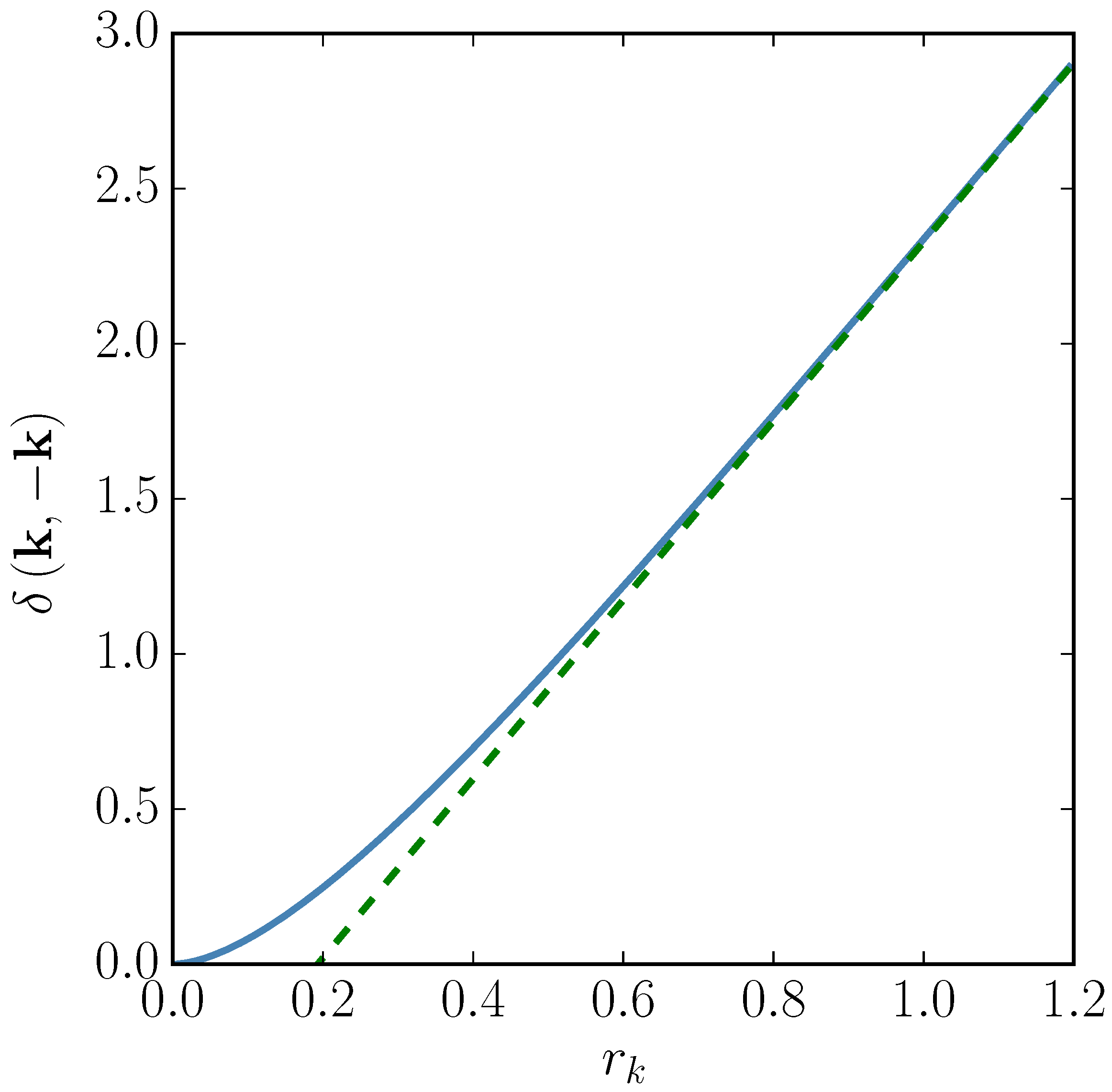
Having defined what the quantum discord is, one can now calculate it for a two-mode squeezed state. Straightforward manipulations lead to [23]

$$\begin{array}{c}\hfill \delta (\mathit{k},-\mathit{k})={cosh}^2{r}_k{log}_2\left({cosh}^2{r}_k\right)-{sinh}^2{r}_k{log}_2\left({sinh}^2{r}_k\right).\end{array}$$

(59)

Let us notice that the discord does not depend on the squeezing angle. The discord is represented in Figure 2. For a vanishing squeezing parameter, the discord is zero and then grows with $r_k$. For large values of $r_k$, it simply grows linearly since $\delta (\mathit{k},-\mathit{k})=2r_k/ln2-2-1/ln2+\mathcal{O}\left(e^{-2r_k}\right)$. Therefore, one concludes that a two-mode squeezed state is not a classical state at all, at least if one accepts the quantum discord as a meaningful criterion for classicality.

4. EPR, EPW and Cosmology

4.1. Negativity of the Wigner Distribution as a Criterion of Non-Classicality

We have reached a seemingly paradoxical stage. On one hand, the considerations in Section 3.1 seem to indicate that the system is classical. Everything can indeed be described by means of a stochastic distribution, namely the Wigner function. This one is positive definite because we deal with a Gaussian state and the Weyl transform of any power of curvature perturbation is “trivial”, which indicates that any quantum correlation function can be obtained as a stochastic correlation function using the Wigner distribution. On the other, a two-mode squeezed state tends to an EPR state and, moreover, modern criterion designed in the context of Quantum Information Theory, such as the quantum discord calculated in the last section, Section 3.2, unambiguously shows that the system is quantum. How can we understand something which, at first sight, looks like a contradiction? It should be added that, although interesting in general, this question is especially relevant in Cosmology which, as argued before, is the situation in Physics where the strongest squeezing and, therefore, the largest discord, are obtained.

In fact, this question has a fascinating history although it was realized only very recently that Cosmology is probably the most interesting context to discuss it. To our knowledge, it started in 1986 with the letter “EPR correlations and EPW distributions” [27] that J. Bell presented in a conference organized by the New York Academy of Sciences and which is also reproduced in his famous book “Speakable and unspeakable in quantum mechanics” (this is chapter 21) [28]. The letters “EPW” in the title stand for “Eugene Paul Wigner” since Bell’s letter is dedicated to Professor E. P. Wigner. Amusingly enough, the inflationary mechanism for structure formation was invented only a few years before and, soon after Bell’s letter, in 1990, Grishchuk and Sidorov [29] realized for the first time that a two-mode squeezed state was involved in the inflationary scenario. Remarkably, the Grishchuk and Sidorov paper contains a calculation of the Wigner function of cosmological perturbations.

The main idea of Bell’s paper is to relate the presence of non-classical, quantum, correlations to the non-positivity of the Wigner function. The idea that a negative Wigner function signals non-classicality is intuitive since a classical probability function must be positive. It is best illustrated in the case of a Schrödinger cat state (we consider for simplicity but without loss of generality, a one-dimensional system)

$$\begin{array}{c}\hfill {\Psi }_{\mathrm{CAT}}\left(q\right)=\frac{N_{\mathrm{CAT}}}{\sqrt{2}}\left[{\Phi }_{+}\left(q\right)+{\Phi }_{-}\left(q\right)\right],\end{array}$$

(60)

with

$$\begin{array}{c}\hfill {\Phi }_{\pm }\left(q\right)={\left(\frac{m\omega }{\pi }\right)}^{1/4}exp\left[-\frac{m\omega }{2}{(q\pm q_0)}^2+i{p}_0(q\pm q_0)\right],\end{array}$$

(61)

and $N_{\mathrm{CAT}}={[1+e^{-m\omega q_0^2}cos\left(2q_0{p}_0\right)]}^{-1/2}$ in order for the wave function (60) to be properly normalized. Inserting this expression into the definition of the Wigner function, 2 one arrives at the following expression (see Ref. [47])

$$\begin{array}{c}\hfill W_{\mathrm{CAT}}(q,p)=W_{+}(q,p)+W_{-}(q,p)+W_{\mathrm{int}}(q,p),\end{array}$$

(63)

where $W_{\pm }(q,p)$ represents the Wigner function of a single wave packet, namely

$$\begin{array}{c}\hfill W_{\pm }(q,p)=\frac{N_{\mathrm{CAT}}^2}{2\pi }{e}^{-m\omega {(q\pm q_0)}^2-\frac{1}{m\omega }{(p-p_0)}^2},\end{array}$$

(64)

and $W_{\mathrm{int}}(q,p)$ is an interaction term

$$\begin{array}{c}\hfill W_{\mathrm{int}}(q,p)=\frac{N_{\mathrm{CAT}}^2}{\pi }cos\left(2p{q}_0\right)e^{-m\omega q^2-\frac{1}{m\omega }{(p-p_0)}^2}.\end{array}$$

(65)

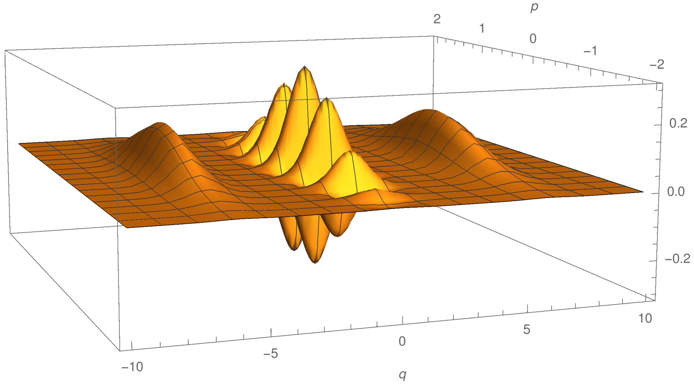
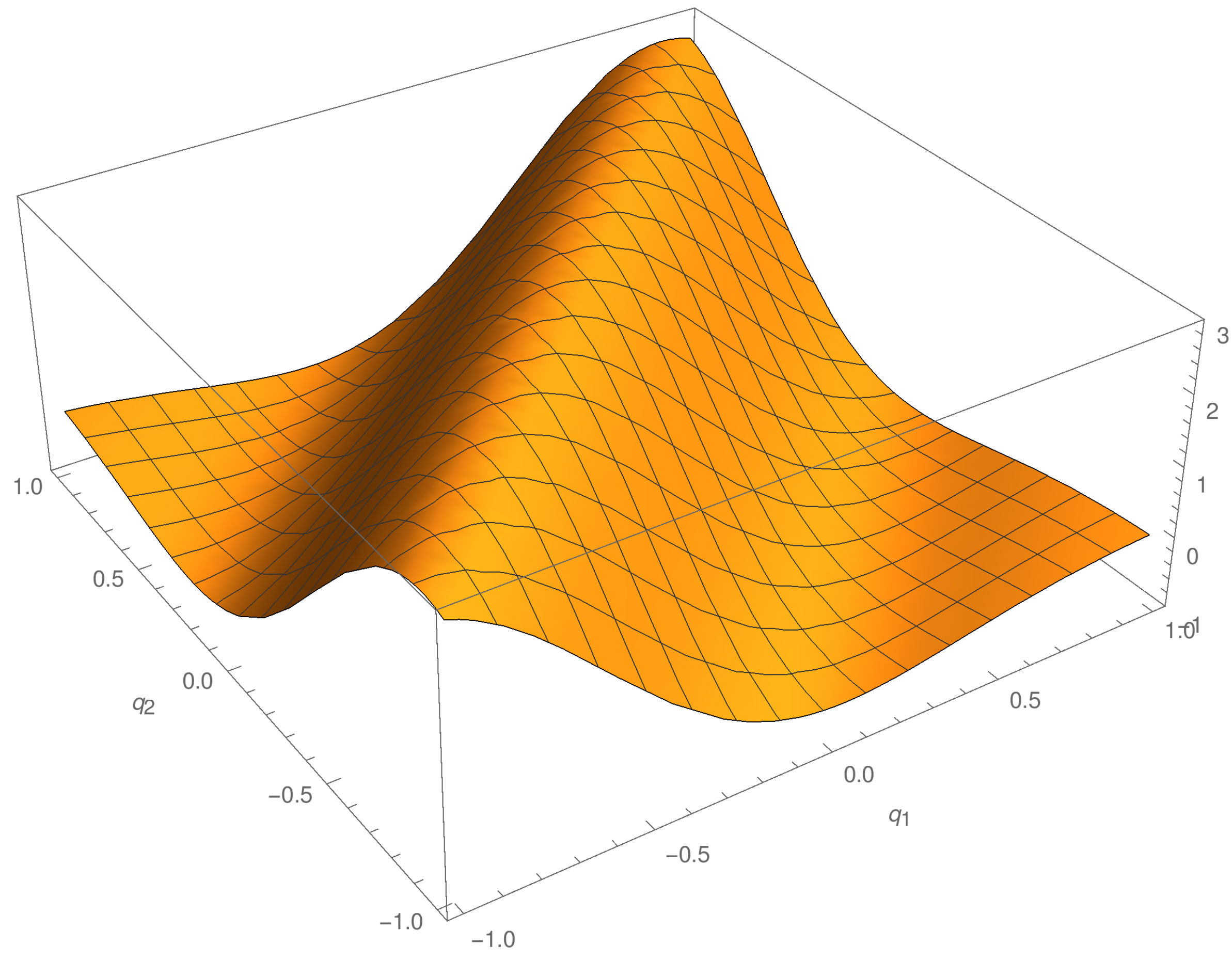
This Wigner function is represented in Figure 3. We see two peaks where the Wigner function is positive and, in between, a series of oscillations due to the cosine term in Equation (65) where the Wigner function can be negative. The oscillations in the Wigner function are clearly due to interferences between the two wave packets. Therefore, interferences, which are a typical quantum phenomenon, are responsible for the non-positivity of the Wigner function, hence the idea to view the non-positivity of the Wigner function as a criterion for classicality.

4.2. WKB

Given the considerations presented in the previous section, it is interesting to calculate the Wigner function of a WKB state since the WKB approximation is often viewed as a way to study the classical limit in Quantum Mechanics. Surprisingly, the calculation of the WKB Wigner function is not as straightforward as one might think at first sight. In Cosmology, it has even a controversial and rich history. The WKB Wigner function has indeed been applied to various questions in Cosmology such as the interpretation of the wavefunction of the Universe (Quantum Cosmology) and the quantum-to-classical transition of inflationary perturbations, this last topic being obviously especially relevant for the present article.

Although the original calculation of the semi-classical Wigner function was performed by M. Berry in 1976 [48], it started to be applied in Cosmology only at the end of the 1980s in Ref. [49]. The question of how to interpret the wavefunction of the Universe in Quantum Cosmology was the issue tackled in this article. Usually, the solution of the Wheeler-de Witt equation makes sense only in the WKB approximation because this is the regime where positive probabilities can be extracted from this formalism (recall that the Wheeler–de Witt equation is similar to a Klein–Gordon equation and, hence, does not always lead to positive probabilities). Then, the idea was to look for correlations in the WKB Wigner function. The calculation of Ref. [49] proceeds as follows. Inserting the WKB wavefunction,

$$\begin{array}{c}\hfill \Psi (q,t)=C(q,t)exp\left[\frac{i}{\hslash }S(q,t)\right],\end{array}$$

(66)

where we have provisionally re-established ℏ and where $S(q,t)$ is the classical action of the system, into the definition of the Wigner function, one arrives at

$$\begin{array}{c}\hfill W_{\mathrm{WKB}}(q,p)=\frac{1}{2\pi \hslash }\int \mathrm{d}x{C}^{\ast }\left(q-\frac{1}{2}\hslash x\right)C\left(q+\frac{1}{2}\hslash x\right)exp\left[-\frac{i}{\hslash }px-\frac{i}{\hslash }S\left(q-\frac{1}{2}\hslash x\right)+\frac{i}{\hslash }S\left(q+\frac{1}{2}\hslash x\right)\right].\end{array}$$

(67)

Expanding the amplitude and the phase in ℏ, one obtains

$$\begin{array}{c}\hfill W_{\mathrm{WKB}}(q,p)\simeq \frac{1}{2\pi \hslash }\int \mathrm{d}x\left[{\left|C\left(q\right)\right|}^2+\mathcal{O}\left({\hslash }^2\right)\right]exp\left[-\frac{i}{\hslash }px+\frac{i}{\hslash }\frac{\partial S}{\partial q}x+\mathcal{O}\left({\hslash }^2\right)\right],\end{array}$$

(68)

that is to say, by performing the integration over x

$$\begin{array}{c}\hfill W_{\mathrm{WKB}}(q,p)={\left|C\left(q\right)\right|}^2\delta \left(p-\frac{\partial S}{\partial q}\right).\end{array}$$

(69)

Therefore, the conclusion of Ref. [49] was that the WKB approximation is really a classical limit in the sense that the Wigner function is positive definite and peaked over the classical trajectories $p=\partial S/\partial q$ with a weight given by the squared amplitude ${\left|C\left(q\right)\right|}^2$.

However, after the publication of Ref. [49], it was pointed out in Refs. [50,51] that the calculation of the WKB Wigner function (69) is in fact unjustified and that, moreover, the correct formula was derived, as already mentioned, by M. Berry in Ref. [48]. The trouble with Equation (69) is that one cannot truncate the expansion of the phase and, then, perform the integration over x. It is true that the higher order terms are proportional to powers of ℏ (which goes to zero) but also to powers of x (the range of which is the entire real axis) so that it is unclear whether the contributions of higher order terms are really negligible. The correct method consists in fact in using the saddle point approximation. This leads to

$$\begin{array}{c}\hfill W_{\mathrm{WKB}}(q,p)=2\sqrt{2}\frac{{\left[\frac{3}{2}A(q,p)\right]}^{1/6}}{{\left[\frac{\partial E}{\partial q}{|}_2\frac{\partial E}{\partial p}{|}_1-\frac{\partial E}{\partial p}{|}_2\frac{\partial E}{\partial q}{|}_1\right]}^{1/2}}\mathrm{Ai}\left\{-{\left[\frac{3}{2}A(q,p)\right]}^{2/3}\right\},\end{array}$$

(70)

where $\mathrm{Ai}\left(z\right)$ is a Airy function [52]. In the above expression, E is the energy shell, namely the quantity such that the Hamiltonian of the system satisfies $H(p,q)=E$. The points 1 and 2 are the points of coordinates $q\pm x_0(q,p)$, $p(q\pm x_0)$ satisfying the stationary phase condition $\left[p\left(q-x_0/2,E\right)+p\left(q+x_0/2,E\right)\right]=2p$. They lie on the classical trajectory and their position is determined such that the arithmetic mean of their momentum is p. Finally, $A(q,p)$ is the area comprised between the chords 1–2 and the classical torus $H=E$. One can show that, when the Wigner function is known, the above formula (70) matches very well the exact result in the regime where the WKB condition is valid. However, the most important property of Equation (70) is that it is not positive definite and usually displays oscillations in phase space. This shows that the semi-classical limit cannot be viewed as being a truly classical regime.

The WKB approximation has also been applied to the quantum-to-classical transition of cosmological perturbations in Ref. [53]. In that paper, it is claimed that this transition is achieved because the quantum state of the perturbations precisely satisfies the WKB approximation on super Hubble scales. Based on what we have just seen about the WKB Wigner function, this last statement should be taken with great care. In fact, as we are going to see, the behavior of cosmological perturbations on large scales is especially relevant when it comes to semi-classical methods in phase space.

Based on the fact that the quantum state of the perturbations is a squeezed state, Ref. [53] considers a simplified model consisting in an inverted harmonic oscillator whose Lagrangian is given by

$$\begin{array}{c}\hfill L=\frac{1}{2}m{\dot{q}}^2+\frac{1}{2}k{q}^2,\end{array}$$

(71)

where the potential term has the “wrong” sign, $V\left(x\right)=-k{q}^2/2$. As we are going to see, the state of the oscillator evolves into a strongly squeezed state which justifies considering this simple system. The corresponding Hamiltonian reads $H=p^2/\left(2m\right)-k{q}^2/2$, with $p=\partial L/\partial \dot{q}=m\dot{q}$, and is not bounded from below. Then, creation and annihilation operators can be introduced in the standard fashion

$$\begin{array}{c}\hfill \widehat{q}=\sqrt{\frac{1}{2m\omega }}\left(\widehat{c}+{\widehat{c}}^{†}\right),\widehat{p}=-i\sqrt{\frac{m\omega }{2}}\left(\widehat{c}-{\widehat{c}}^{†}\right),\end{array}$$

(72)

where ${\omega }^2=k/m$. This allows us to express the Hamiltonian as

$$\begin{array}{c}\hfill \widehat{H}=-\frac{\omega }{2}\left({\widehat{c}}^2+{\widehat{c}}^{†2}\right).\end{array}$$

(73)

Of course, the most striking property of this Hamiltonian is the presence of an overall minus sign which is just the consequence of the inverted nature of the oscillator. Then, the equations of motion are given by

$$\begin{array}{c}\hfill \frac{\mathrm{d}\widehat{c}}{\mathrm{d}t}=-i\left[\widehat{c},\widehat{H}\right]=i\omega {\widehat{c}}^{†},\frac{\mathrm{d}{\widehat{c}}^{†}}{\mathrm{d}t}=-i\left[{\widehat{c}}^{†},\widehat{H}\right]=-i\omega \widehat{c}.\end{array}$$

(74)

As usual, they can be solved by mean of a Bogoliubov transformation, namely

$$\begin{array}{c}\hfill \widehat{c}\left(t\right)=u\left(t\right)\widehat{c}(t_{\mathrm{ini}})+v\left(t\right){\widehat{c}}^{†}(t_{\mathrm{ini}}),{\widehat{c}}^{†}\left(t\right)=u^{\ast }\left(t\right){\widehat{c}}^{†}\left(t_{\mathrm{ini}}\right)+v^{\ast }\left(t\right)\widehat{c}(t_{\mathrm{ini}}),\end{array}$$

(75)

where the functions $u\left(t\right)$ and $v\left(t\right)$ satisfy the following equations:

$$\begin{array}{c}\hfill \frac{\mathrm{d}u}{\mathrm{d}t}=i\omega v^{\ast },\frac{\mathrm{d}v}{\mathrm{d}t}=i\omega u^{\ast },\end{array}$$

(76)

with initial conditions $u\left(0\right)=1$ and $v\left(0\right)=0$ (here, for simplicity, we have taken $t_{\mathrm{ini}}=0$). Combining these two first order differential equations, one can obtain one second order equation for u (and/or v), which reads

$$\begin{array}{c}\hfill \frac{{\mathrm{d}}^{2}u}{\mathrm{d}{t}^2}={\omega }^{2}u,\end{array}$$

(77)

which gives $u\left(t\right)=cosh\left(\omega t\right)$ and $v\left(t\right)=isinh\left(\omega t\right)$. As a consequence, the operator $\widehat{c}\left(t\right)$ can be rewritten as

$$\begin{array}{c}\hfill \widehat{c}\left(t\right)=cosh\left(\omega t\right){\widehat{c}}_{\mathrm{ini}}+e^{i\pi /2}sinh\left(\omega t\right){\widehat{c}}_{\mathrm{ini}}^{†}={\widehat{S}}^{†}{\widehat{c}}_{\mathrm{ini}}\widehat{S},\end{array}$$

(78)

where we have written $\widehat{c}(t_{\mathrm{ini}})=\widehat{c}$ and where the operator $\widehat{S}$ is defined by

$$\begin{array}{c}\hfill \widehat{S}=exp\left[\frac{r}{2}\left({\widehat{c}}_{\mathrm{ini}}^2{e}^{-2i\varphi }-{\widehat{c}}_{\mathrm{ini}}^{†}2e^{2i\varphi }\right)\right],\end{array}$$

(79)

with squeezing parameter and angle given by $r=\omega t$ and $\varphi =-\pi /4$. $\widehat{S}$ is the squeezing operator and is responsible, as announced above, for the appearance of squeezed states in the problem.

In order to mimic the behavior of cosmological perturbations, we assume that the initial state of the system is the vacuum $|0\rangle$. Then, the state at a subsequent time t can be found using techniques based on the operator ordering theorem [54], which allows us to rewrite the operator $\widehat{S}$ as

$$\begin{array}{c}\hfill \widehat{S}=exp\left[e^{-2i\varphi }tanh\left|r\right|\frac{{{\widehat{c}}_{\mathrm{ini}}^{†}}^2}{2}\right]exp\left[-\frac{1}{2}({\widehat{c}}_{\mathrm{ini}}{\widehat{c}}_{\mathrm{ini}}^{†}+{\widehat{c}}_{\mathrm{ini}}^{†}{\widehat{c}}_{\mathrm{ini}})ln(cosh|r\left|\right)\right]exp\left[-e^{2i\varphi }tanh\left|r\right|\frac{{\widehat{c}}_{\mathrm{ini}}^2}{2}\right],\end{array}$$

(80)

from which it follows that

$$\begin{array}{c}\hfill |\Psi \rangle =\widehat{S}|0\rangle =\frac{1}{\sqrt{coshr}}{\displaystyle \sum _{p=0}^{\infty }}\frac{e^{-2ip\varphi }}{2^{p}p!}\sqrt{2p!}{tanh}^{p}r|2p\rangle .\end{array}$$

(81)

This state is a one-mode squeezed state. It slightly differs from the two-mode squeezed state considered before in Equation (21). In particular, we see that the sum is only on states with an even number of particles. Since $r=\omega t$, the squeezing goes to infinity in the large time limit.

Our next move is to calculate the wavefunction. It reads

$$\begin{array}{c}\hfill \Psi \left(q\right)=〈q|\Psi 〉=\frac{e^{-q^2/2}}{{\pi }^{1/4}\sqrt{coshr}}{\displaystyle \sum _{p=0}^{\infty }}\frac{e^{-2ip\varphi }}{2^{2p}p!}{tanh}^{p}r{H}_{2p}\left(q\right),\end{array}$$

(82)

where $H_{2p}\left(z\right)$ is a Hermite polynomial of order $2p$ [52] and appears in the q-representation of the state $|2p\rangle$. Then, using ${\sum }_{p=0}^{\infty }{t}^n{H}_{2n}\left(x\right)/n!=e^{4t{x}^2/(1+4t)}/\sqrt{1+4t}$ (here, one has $4t=e^{-2i\varphi }tanhr$) and, recalling that $\varphi =-\pi /4$, one arrives at

$$\begin{array}{c}\hfill \Psi \left(q\right)={\left[\pi cosh\left(2r\right)\right]}^{-1/4}exp\left[-\frac{q^2}{2cosh\left(2r\right)}+\frac{i}{2}{q}^{2}tanh\left(2r\right)-\frac{i}{2}arctan\left(tanhr\right)\right],\end{array}$$

(83)

where one verifies that this wavefunction is correctly normalized.

As noticed in Ref. [53], it can be written in a WKB form (66) with

$$\begin{array}{c}\hfill C={\left[\pi cosh\left(2r\right)\right]}^{-1/4}exp\left[-\frac{q^2}{2cosh\left(2r\right)}\right],S=\frac{1}{2}{q}^{2}tanh\left(2r\right)-\frac{1}{2}arctan\left(tanhr\right),\end{array}$$

(84)

and, in the large time limit or, equivalently, strong squeezing limit, the semi-classical approximation is extremely well-verified since the WKB condition is satisfied $|C{\partial }_{q}S/{\partial }_{q}C|=sinh\left(2r\right)\gg 1$. Hence, the claim that cosmological perturbations on super Hubble scales, which is equivalent to strong squeezing, are “semi-classical”. It is then tempting to go from “semi-classical” to “classical” and consider that the quantum-to-classical transition has been achieved. However, as seen above, given that the WKB Wigner function is not positive definite, one should a priori resist to this temptation.

However, as it is often the case, Cosmology introduces a new twist in this question. Using Equation (83), one can calculate the Wigner function. The result reads

$$\begin{array}{c}\hfill W(q,p)=\frac{1}{\pi }{e}^{-q^2/cosh\left(2r\right)}{e}^{-cosh\left(2r\right){\left[p-qtanh\left(2r\right)\right]}^2}.\end{array}$$

(85)

One obtains a Gaussian, which is consistent with the fact that the wavefunction (83) is a Gaussian. This means that this Wigner function, contrary to the WKB Wigner function (70), is positive definite, which, at first sight, seems surprising since $\Psi \left(q\right)$ in Equation (83) satisfies the WKB approximation. Moreover, writing $ϵ=1/[4cosh(2r\left)\right],$ which, in the strong squeezing limit, goes to zero, representing the Dirac function by ${\delta }_{ϵ}\left(x\right)=e^{-x^2/\left(4ϵ\right)}/\left[2\sqrt{\pi ϵ}\right]$ and, finally, noticing that $p=\partial S/\partial q=qtanh\left(2r\right)$, the Wigner function (85) can be re-written as

$$\begin{array}{c}\hfill W(q,p)={\left|C\right|}^2{\delta }_{ϵ}\left[p-qtanh\left(2r\right)\right]={\left|C\right|}^2{\delta }_{ϵ}\left(p-\frac{\partial S}{\partial q}\right),\end{array}$$

(86)

where C is given in Equation (84). This equation is nothing but Equation (69) which was, as discussed in Refs. [50,51], supposed to be incorrect! What happened is in fact very simple. It was pointed out before that the expansion of the phase performed in Ref. [49] is not justified because the order of the various terms of this expansion is in fact indeterminate. There is of course one exception to this claim which is when the calculation of Ref. [49] is not an expansion but is exact. This is exactly what happens here since the phase is quadratic in q. Thus, ignoring higher order terms, which is usually unjustified, is, in the present case, totally valid simply because these higher order terms are just not present. This is consistent with the fact that the Wigner function of Gaussian is a Gaussian and, therefore, is positive definite. This shows how peculiar and subtle is the quantum-to-classical transition of cosmological perturbations is.

4.3. Bell’s Paper on the Wigner Function

After these preliminary considerations, let us now come back to the letter written by J. Bell in 1986 [27]. Based on the original EPR article [43], Bell imagines a situation where there are two free particles traveling in space along a given axis (the particles can propagate in both directions). Then, Bell assumes that one can measure position (of the two particles) only. As he notices himself, this slightly differs from the standard EPR argument where it is also assumed that momenta can be measured. The article makes use of the “two-time” Wigner function defined by

$$\begin{array}{cc}\hfill W(q_1,q_2,p_1,p_2,t_1,t_2)& =\frac{1}{{\left(2\pi \right)}^2}\int \mathrm{d}{y}_1\mathrm{d}{y}_2{e}^{-i{p}_1{y}_1-i{p}_2{y}_2}\hfill \\ & \times \Psi \left(q_1+\frac{y_1}{2},q_2+\frac{y_2}{2},t_1,t_2\right){\Psi }^{\ast }\left(q_1-\frac{y_1}{2},q_2-\frac{y_2}{2},t_1,t_2\right),\hfill \end{array}$$

(87)

where $\Psi (q_1,q_2,t_1,t_2)$ is the wavefunction of the system. If one considers two freely-moving particles, then $\Psi$ satisfies the Schrödinger equations, $i\partial \Psi /\partial t_{1,2}={\widehat{p}}_{1,2}^2/\left(2m_{1,2}\right)\Psi$ and, as a consequence, the Wigner function obeys $(\partial /\partial t_{1,2}+p_{1,2}\partial /\partial q_{1,2})W=0$. This means that $W(q_1,q_2,p_1,p_2,t_1,t_2)=W(q_1-p_1{t}_1,q_2-p_2{t}_2,p_1,p_2,0,0)$ and this allows us to calculate the Wigner function at any times from the sole knowledge of the initial wavefunction. Of course, the calculation of $W(q_1-p_1{t}_1,q_2-p_2{t}_2,p_1,p_2,0,0)$ still requires the knowledge of the wavefunction and, in the following, several possibilities are considered.

Then, Bell proceeds and shows how his famous inequality can be implemented in the situation described before. More precisely, he does so in the so-called Clauser, Horne, Shimony and Holt (CHSH) formulation3, which supposes to deal with quantities that can only take the values $\pm 1$. This is why, usually, the CHSH inequality is experimentally tested with spin variables. However, in the case considered by Bell, the particles are spinless and, as already mentioned, we only have access to position measurements. Although he does not present it exactly in this way, what Bell does to circumvent this problem is to introduce the two following operators:

$$\begin{array}{c}\hfill {\widehat{S}}_1\left(t_1\right)=\mathrm{sgn}\left({\widehat{q}}_1+\frac{q_0}{2},t_1\right),{\widehat{S}}_2\left(t_2\right)=\mathrm{sgn}\left({\widehat{q}}_2-\frac{q_0}{2},t_2\right),\end{array}$$

(88)

which represent the sign of $q_1+q_0/2$ and $q_2-q_0/2$ at times $t_1$ and $t_2$, respectively, $q_0$ being an arbitrary position. Clearly, the spectra of ${\widehat{S}}_1$ and ${\widehat{S}}_2$ only consist of two values, namely $\pm 1$, as required. Interestingly enough, this is exactly what is done in Refs. [56,57,58] and, then in the context of Cosmology, in Refs. [25,26]. Therefore, remarkably, Bell’s paper already contains the idea of fictitious spin operators that, as we will see later on, can be used in order to design a cosmic Bell experiment.

Then, once we have discrete variables, one can just mimic the usual approach, which, as reminded above, is formulated in terms of spins. The first step consists of defining the two-point correlators

$$\begin{array}{c}\hfill E(t_1,t_2)\equiv 〈\Psi \left|{\widehat{S}}_1\left(t_1\right){\widehat{S}}_2\left(t_2\right)\right|\Psi 〉,\end{array}$$

(89)

where $|\Psi \rangle$ is the quantum state in which the system is placed. Let us also remark that the two times $t_1$ and $t_2$ play the role of the polarizers settings in the standard CHSH formulation. Following the usual considerations, one can then prove that

$$\begin{array}{c}\hfill B(t_1,t_2,t_1^{\prime },t_2^{\prime })=E(t_1,t_2)+E(t_1,t_2^{\prime })+E(t_1^{\prime },t_2)-E(t_1^{\prime },t_2^{\prime })\le 2,\end{array}$$

(90)

if the correlators are interpreted as stochastic averages and if locality holds [59]. On the contrary, in Quantum Mechanics, one just has $B(t_1,t_2,t_1^{\prime },t_2^{\prime })<2\sqrt{2}$, hence the idea to look for experimental configurations for which $2<B(t_1,t_2,t_1^{\prime },t_2^{\prime })<2\sqrt{2}$. In the following, Bell inequality violation (or CHSH inequality violation, we use the two expressions indifferently) will refer to as a situation where $B(t_1,t_2,t_1^{\prime },t_2^{\prime })>2$.

As discussed at the beginning of this section, Bell wants to relate the non-positivity of the Wigner function to a violation of the CHSH inequality. Technically, the link between the inequality and the Wigner function is expressed as follows. It is easy to check that the quantities $S_1$ and $S_2$ are such that $\widetilde{S_1}=S_1$ and ${\tilde{S}}_2=S_2$—see the discussion above in Section 3.1—and, as a consequence, thanks to Equations (43) and (44), the expression of the correlator $E(t_1,t_2)$ can be rewritten as

$$\begin{array}{cc}\hfill E(t_1,t_2)& ={\int }_{-\infty }^{\infty }\mathrm{d}{q}_1{\int }_{-\infty }^{\infty }\mathrm{d}{q}_2{\int }_{-\infty }^{\infty }\mathrm{d}{p}_1{\int }_{-\infty }^{\infty }\mathrm{d}{p}_{2}W(q_1,q_2,p_1,p_2,t_1,t_2){\tilde{S}}_1\left(t_1\right){\tilde{S}}_2\left(t_2\right)\hfill \end{array}$$

(91)

$$\begin{array}{c}={\int }_{-\infty }^{\infty }\mathrm{d}{q}_1{\int }_{-\infty }^{\infty }\mathrm{d}{q}_2{\int }_{-\infty }^{\infty }\mathrm{d}{p}_1{\int }_{-\infty }^{\infty }\mathrm{d}{p}_{2}W(q_1-p_1{t}_1,q_2-p_2{t}_2,p_1,p_2,0,0){\tilde{S}}_1\left(t_1\right){\tilde{S}}_2\left(t_2\right)\hfill \end{array}$$

(92)

$$\begin{array}{c}\hfill ={\int }_{-\infty }^{\infty }\mathrm{d}{q}_1{\int }_{-\infty }^{\infty }\mathrm{d}{q}_2{\tilde{S}}_1\left(t_1\right){\tilde{S}}_2\left(t_2\right)\rho (q_1,q_2,t_1,t_2),\end{array}$$

(93)

where the two-time distribution probability $\rho (q_1,q_2,t_1,t_2)$ is defined by $\rho (q_1,q_2,t_1,t_2)={\int }_{-\infty }^{\infty }\mathrm{d}{p}_1{\int }_{-\infty }^{\infty }\mathrm{d}{p}_{2}W(q_1-p_1{t}_1,q_2-p_2{t}_2,p_1,p_2,0,0)$. The above equations exactly represent the relation needed as it allows us to estimate the left-hand side of Equation (90) in terms of the Wigner function. Using the definition of ${\tilde{S}}_1$ and ${\tilde{S}}_2$, one can also show that

$$\begin{array}{cc}\hfill E(t_1,t_2)& =1-2[{\int }_0^{+\infty }\mathrm{d}{\overline{q}}_1{\int }_{-\infty }^0\mathrm{d}{\overline{q}}_2\rho \left({\overline{q}}_1-\frac{q_0}{2},{\overline{q}}_2+\frac{q_0}{2},t_1,t_2\right)\hfill \\ & +{\int }_{-\infty }^0\mathrm{d}{\overline{q}}_1{\int }_0^{+\infty }\mathrm{d}{\overline{q}}_2\rho \left({\overline{q}}_1-\frac{q_0}{2},{\overline{q}}_2+\frac{q_0}{2},t_1,t_2\right)],\hfill \end{array}$$

(94)

where we used the fact that the Wigner function is normalized to one.

To go further and concretely calculate the correlators, and, hence, verify whether the CHSH inequality is violated or not, one needs to specify the state in which the system is placed. The first example considered by Bell is simply the original EPR wavefunction [43] (supposed to hold at initial times), ${\Psi }_{\mathrm{EPR}}(q_1,q_2)=N_{\mathrm{EPR}}\delta (q_1-q_2+q_0)$, where $N_{\mathrm{EPR}}$ is a normalization constant. Then, he calculates the corresponding Wigner function and finds

$$\begin{array}{c}\hfill W_{\mathrm{EPR}}(q_1,q_2,p_1,p_2,0,0)=\frac{N_{\mathrm{EPR}}^2}{4\pi }\delta (q_1-q_2+q_0)\delta (p_1+p_2).\end{array}$$

(95)

Bell remarks that this Wigner function is positive everywhere and that “the EPR correlations are precisely those between two classical particles in independent free classical motion. With the wave function (8) (namely the EPR wavefunction), then, there is no non-locality problem when the incompleteness of the wave function description is admitted”. Therefore, Bell explicitly relates classicality (namely no violation of the CHSH inequality) and positivity of the Wigner function.

However, it is interesting to notice that he does not explicitly verify the violation of the CHSH inequality in that case (namely, he does not explicitly calculate the two-point correlators for the EPR wavefunction nor the combination (90)), despite the fact that he clearly suggests it is not violated. Although he does not explain why, one can maybe guess the reason. If one takes the EPR Wigner function (95) and tries to calculate $\rho (q_1,q_2,t_1,t_2),$ one finds an infinite result. Indeed, the first integration, say on $p_1$, kills the Dirac delta function $\delta (p_1+p_2)$. Then, it remains an integral over $p_2$ of something which does not depend on $p_2$, which gives an infinite result. This remark is interesting because it turns out to be at the core of all the literature that is devoted to this question and to the Bell’s paper: this will be discussed at length in the following sections. The reason for this problem is in fact related to the normalization $N_{\mathrm{EPR}}$. Indeed, the wavefunction ${\Psi }_{\mathrm{EPR}}(q_1,q_2)$ is not properly normalized. A correct way to normalize it is to modify the wavefunction such that it now reads

$$\begin{array}{c}\hfill {\Psi }_{\mathrm{EPR}}(q_1,q_2)={\left(\frac{\epsilon }{b}2\sqrt{2}\right)}^{1/2}{e}^{-{(q_1+q_2)}^2/\left(2b^2\right)}\frac{1}{\epsilon \sqrt{\pi }}{e}^{-{(q_1-q_2+q_0)}^2/{\epsilon }^2}.\end{array}$$

(96)

This is suggested by Bell himself in the continuation of his article. Strictly speaking, in Bell’s paper, this trick is not applied to the EPR wavefunction but to another wavefunction considered later on in his article (and, in the present paper as well, see Equation (108)). Here, we have just anticipated his guess and have applied it to the EPR wavefunction. We will comment more about this point in the following. The “new” wavefunction (96) is made of three pieces: a normalization factor, a new factor depending on a new parameter b, $e^{-{(q_1+q_2)}^2/\left(2b^2\right)}$ and the last factor depending on another new parameter $\epsilon$, $e^{-{(q_1-q_2+q_0)}^2/{\epsilon }^2}/\left(\epsilon \sqrt{\pi }\right)$. This last factor is just a finite representation of the Dirac function $\delta (q_1-q_2+q_0),$ which is recovered in the limit $\epsilon \to 0$. The second factor is necessarily present to make the wavefunction normalizable. Even if one uses the finite representation of the Dirac function, it is not possible to make $\int |{\Psi }_{\mathrm{EPR}}{|}^2\mathrm{d}{q}_1\mathrm{d}{q}_2$ finite without the factor $e^{-{(q_1+q_2)}^2/\left(2b^2\right)}$ as it is easy to see by introducing new variables $q_1\pm q_2$ in the previous integral. Finally, the first factor is the normalization coefficient implied by the two other factors.

In his article, Bell claims 4 that the second factor can be ignored by taking the limit $b\to \infty$. However, we see that this limit, as well as the limit $\epsilon \to 0$, are very problematic due to the normalization factor. For this reason, in the following, we work with Equation (96) without taking any limit. Since the wavefunction is Gaussian, the calculations are tractable. Indeed, using the wavefunction (96), it is easy to calculate the Wigner function, which reads

$$\begin{array}{c}\hfill W_{\mathrm{EPR}}(q_1,q_2,p_1,p_2,0,0)=\frac{1}{{\pi }^2}{e}^{-b^2{(p_1+p_2)}^2/4-{(q_1+q_2)}^2/b^2}{e}^{-{\epsilon }^2{(p_1-p_2)}^2/8-2{(q_1-q_2+q_0)}^2/{\epsilon }^2}.\end{array}$$

(97)

Of course, since the state (96) is Gaussian, we find that the Wigner function is also a Gaussian—see Section 2.5. One checks that the Wigner function is properly normalized, $\int \mathrm{d}{q}_1\mathrm{d}{q}_2\mathrm{d}{p}_1\mathrm{d}{p}_2{W}_{\mathrm{EPR}}=1$, which is a consistency check of Equation (97). The next move consists in calculating the distribution $\rho$. Recall that this requires the calculation of $W_{\mathrm{EPR}}(q_1-p_1{t}_1,q_2-p_2{t}_2,p_1,p_2,0,0)$. Using Equation (97), this can be expressed as

$$\begin{array}{c}\hfill W_{\mathrm{EPR}}(q_1-p_1{t}_1,q_2-p_2{t}_2,p_1,p_2,0,0)=\frac{1}{{\pi }^2}{e}^{-{(q_1+q_2)}^2/b^2-2{(q_1-q_2+q_0)}^2/{\epsilon }^2}{e}^{-\frac{1}{2}{P}^{\mathrm{T}}AP-P^{\mathrm{T}}J},\end{array}$$

(98)

where one has defined

$$\begin{array}{cc}\hfill {\displaystyle A}& =\left(\begin{array}{cc}{\displaystyle \frac{b^2}{2}+\frac{{\epsilon }^2}{4}+\left(\frac{2}{b^2}+\frac{4}{{\epsilon }^2}\right)t_1^2}& {\displaystyle \frac{b^2}{2}-\frac{{\epsilon }^2}{4}+\left(\frac{2}{b^2}-\frac{4}{{\epsilon }^2}\right)t_1{t}_2}\\ {\displaystyle \frac{b^2}{2}-\frac{{\epsilon }^2}{4}+\left(\frac{2}{b^2}-\frac{4}{{\epsilon }^2}\right)t_1{t}_2}& {\displaystyle \frac{b^2}{2}+\frac{{\epsilon }^2}{4}+\left(\frac{2}{b^2}+\frac{4}{{\epsilon }^2}\right)t_2^2}\end{array}\right),\hfill \end{array}$$

(99)

and

$$\begin{array}{cc}\hfill J(q_1,q_2)& =\left(\begin{array}{c}{\displaystyle -\frac{2}{b^2}(q_1+q_2)t_1-\frac{4}{{\epsilon }^2}(q_1-q_2+q_0)t_1}\\ {\displaystyle -\frac{2}{b^2}(q_1+q_2)t_2+\frac{4}{{\epsilon }^2}(q_1-q_2+q_0)t_2}\end{array}\right),\hfill \end{array}$$

(100)

and $P^{\mathrm{T}}=(p_1,p_2)$.

Then, the distribution $\rho$ can then be straightforwardly evaluated by applying well-known formula for Gaussian integrals. This leads to

$$\begin{array}{c}\hfill {\rho }_{\mathrm{EPR}}(q_1,q_2,t_1,t_2)=\frac{2}{\pi }{e}^{-{(q_1+q_2)}^2/b^2-2{(q_1-q_2+q_0)}^2/{\epsilon }^2}\frac{1}{\sqrt{detA}}{e}^{\frac{1}{2}{J}^{\mathrm{T}}{A}^{-1}J}.\end{array}$$

(101)

We are now in a position where the correlator $E_{\mathrm{EPR}}(t_1,t_2)$ can be calculated. Plugging the above Equation (101) into Equation (94), one obtains

$$\begin{array}{cc}\hfill E_{\mathrm{EPR}}(t_1,t_2)=& 1-\frac{4}{\pi \sqrt{detA}}[{\int }_0^{+\infty }\mathrm{d}{\overline{q}}_1{\int }_{-\infty }^0\mathrm{d}{\overline{q}}_2{e}^{-{({\overline{q}}_1-q_0/2+{\overline{q}}_2+q_0/2)}^2/b^2-2{({\overline{q}}_1-q_0/2-{\overline{q}}_2-q_0/2+q_0)}^2/{\epsilon }^2}\hfill \\ & \times e^{\frac{1}{2}{J}^{\mathrm{T}}({\overline{q}}_1-q_0/2,{\overline{q}}_2+q_0/2)A^{-1}J({\overline{q}}_1-q_0/2,{\overline{q}}_2+q_0/2)}\hfill \\ & +{\int }_{-\infty }^0\mathrm{d}{\overline{q}}_1{\int }_0^{+\infty }\mathrm{d}{\overline{q}}_2{e}^{-{({\overline{q}}_1-q_0/2+{\overline{q}}_2+q_0/2)}^2/b^2-2{({\overline{q}}_1-q_0/2-{\overline{q}}_2-q_0/2+q_0)}^2/{\epsilon }^2}\hfill \\ & \times e^{\frac{1}{2}{J}^{\mathrm{T}}({\overline{q}}_1-q_0/2,{\overline{q}}_2+q_0/2)A^{-1}J({\overline{q}}_1-q_0/2,{\overline{q}}_2+q_0/2)}].\hfill \end{array}$$

(102)

We see that, in the arguments of all exponentials, $q_0$ cancel out and makes the correlation function independent of $q_0$. This makes sense since this quantity is arbitrary and, therefore, a physical result cannot depend on its value. This also implies that the arguments of the exponentials are in fact quadratic in ${\overline{q}}_1$ and ${\overline{q}}_2$. As a consequence, by a simple change of variable, the second term in the square bracket is in fact equal to the first one. Finally, one obtains

$$\begin{array}{cc}\hfill E_{\mathrm{EPR}}(t_1,t_2)=& 1-\frac{8}{\pi \sqrt{detA}}{\int }_0^{+\infty }\mathrm{d}{\overline{q}}_1{\int }_{-\infty }^0\mathrm{d}{\overline{q}}_2{e}^{c_1{\overline{q}}_1^2+c_2{\overline{q}}_2^2+c_3{\overline{q}}_1{\overline{q}}_2},\hfill \end{array}$$

(103)

where the coefficients $c_1$, $c_2$ and $c_3$ are defined by

$$\begin{array}{cc}\hfill c_1& =-\frac{2b^2+{\epsilon }^2}{2detA}\left(1+\frac{8t_2^2}{b^2{\epsilon }^2}\right),c_2=-\frac{2b^2+{\epsilon }^2}{2detA}\left(1+\frac{8t_1^2}{b^2{\epsilon }^2}\right),c_3=\frac{2b^2-{\epsilon }^2}{detA}\left(1-\frac{8t_1{t}_2}{b^2{\epsilon }^2}\right),\hfill \end{array}$$

(104)

$$\begin{array}{cc}\hfill detA& =\frac{1}{2b^2{\epsilon }^2}\left[b^4{\epsilon }^4+64t_1^2{t}_2^2+(4b^4+{\epsilon }^4){(t_1+t_2)}^4+4b^2{\epsilon }^2{(t_1-t_2)}^2\right].\hfill \end{array}$$

(105)

The integral (103) can easily be performed and one obtains

$$\begin{array}{cc}\hfill E_{\mathrm{EPR}}(t_1,t_2)=& 1-\frac{8}{\pi \sqrt{detA}}\frac{\sqrt{detA}}{8}\left\{\pi -2arctan\left[\frac{(2b^2-{\epsilon }^2)\left[1-8t_1{t}_2/\left(b^2{\epsilon }^2\right)\right]}{4\sqrt{detA}}\right]\right\}\hfill \end{array}$$

(106)

$$\begin{array}{c}=\frac{2}{\pi }arctan\left[\frac{(2b^2-{\epsilon }^2)\left[1-8t_1{t}_2/\left(b^2{\epsilon }^2\right)\right]}{4\sqrt{detA}}\right].\hfill \end{array}$$

(107)

As required, $E_{\mathrm{EPR}}(t_1,t_2)$ varies between $-1$ and 1. It is interesting to notice that the form of the correlator is really typical of what one obtains with pseudo spin operators—see, for instance, Equation (26) of Ref. [26]: the resemblance is striking.

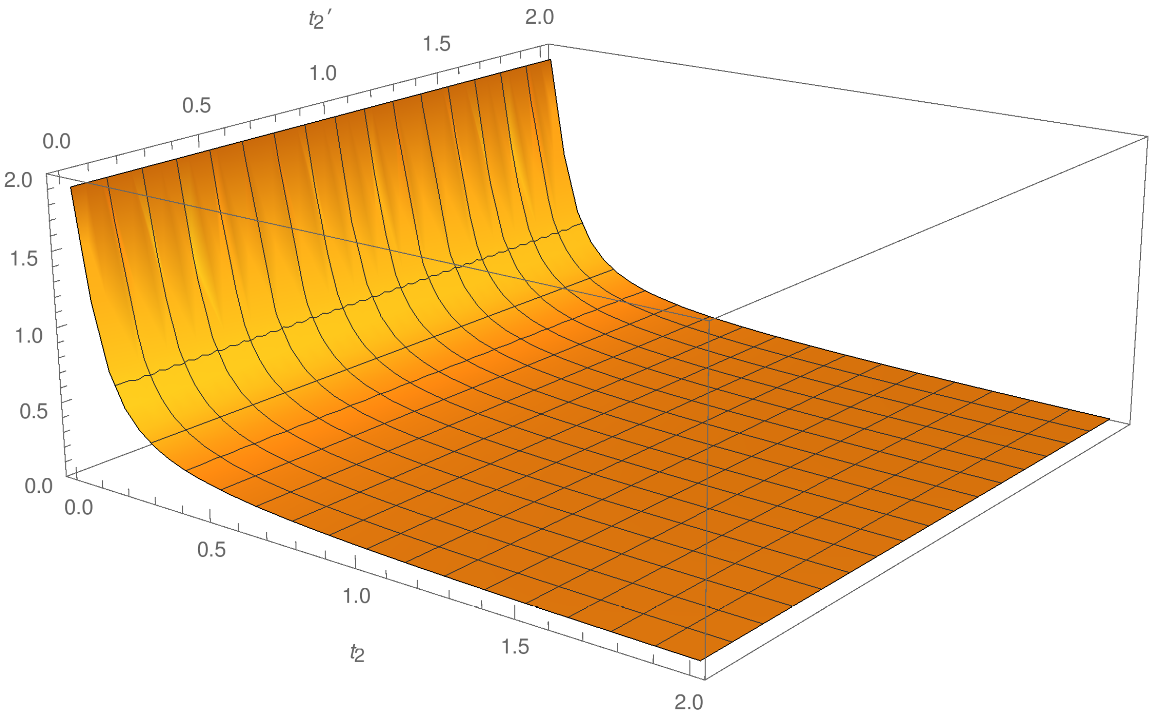
Having obtained the correlators, it is now easy to verify whether the CHSH inequality (90) is violated or not. In Figure 4, we have represented the quantity $B(0,t_2,0,t_2^{\prime })$ defined in Equation (90) and evaluated with the correlator obtained above. We see that this quantity is always smaller than two so that Bell inequality is never violated.

Therefore, we have confirmed Bell’s suggestion that the EPR state, which has a positive Wigner function, does not lead to any Bell inequality violation. This was done with a method that avoided the technical issues present in Bell’s letter. In short, we conclude that Bell calculations are problematic, but, despite those issues, the overall result, at least for the example of the EPR state, is correct.

After this description of the warm-up example in Bell’s paper, we now come to the core of it. As noticed by Bell and as we have seen in detail previously, the EPR state corresponds to a positive Wigner function. However, Bell remarks that this is not always the case and that, for other wavefunctions, the Wigner distribution can take negative values—see, for instance, the case of the Schrödinger cat state (60). The next and crucial step of Bell’s paper is then to study the CHSH inequality for states corresponding to Wigner functions that are not positive definite. In particular, Bell considers the case of the following initial wavefunction

$$\begin{array}{c}\hfill {\Psi }_{\mathrm{BELL}}(q_1,q_2)\propto \left[{\left(q_1-q_2+q_0\right)}^2-2a^2\right]e^{-{(q_1-q_2+q_0)}^2/\left(2a^2\right)},\end{array}$$

(108)

where a is a free parameter. Bell notices that this wavefunction is not properly normalized, but he suggests that it could be easily made so by including a factor $e^{{(q_1+q_2)}^2/\left(2b^2\right)}$, where b is a new parameter 5. Notice that, while only the difference $q_1-q_2$ appeared in Equation (108), considering this extra factor introduces an additional dependence in $q_1+q_2$ in the wavefunction. It can be checked that the wavefunction

$$\begin{array}{c}\hfill {\Psi }_{\mathrm{BELL}}(q_1,q_2)=\sqrt{\frac{8}{11\pi a^{5}b}}\left[{\left(q_1-q_2+q_0\right)}^2-2a^2\right]e^{-{(q_1-q_2+q_0)}^2/\left(2a^2\right)}{e}^{-{(q_1+q_2)}^2/\left(2b^2\right)}\end{array}$$

(109)

is indeed correctly normalized. However, Bells argues that the limit $b\to \infty$ can be taken from the very beginning so that we can work with (108) and ignore the more complicated form (109). The justification given by Bell is that only relative probabilities will be calculated in the rest of his article. Thus, for all practical purposes, he argues that one can work with Equation (108), replacing the proportionality symbol by a $q_1$ and $q_2$ independent “normalization constant” $N_{\mathrm{BELL}}$. In other words, $N_{\mathrm{BELL}}$ which, according to Equation (109), reads $N_{\mathrm{BELL}}=\sqrt{8/\left(11\pi a^{5}b\right)}{e}^{-{(q_1+q_2)}^2/b^2}$, is treated as a simple constant. Then, it is easy to calculate the corresponding Wigner function, which, if the choice $a=1$ is made (namely the value considered by Bell in his letter), reads

$$\begin{array}{cc}\hfill W_{\mathrm{BELL}}(q_1,q_2,p_1,p_2,0,0)& =\frac{N_{\mathrm{BELL}}^2}{\sqrt{\pi }}{e}^{-{(q_1-q_2+q_0)}^2}{e}^{-{(p_1-p_2)}^2/4}[\frac{11}{4}-5{(q_1-q_2+q_0)}^2+{\left(\frac{p_1-p_2}{2}\right)}^2\hfill \\ & +2{\left(\frac{p_1-p_2}{2}\right)}^2{(q_1-q_2+q_0)}^2+{\left(\frac{p_1-p_2}{2}\right)}^4+{(q_1-q_2+q_0)}^4]\delta (p_1+p_2).\hfill \end{array}$$

(110)

This equation is in perfect agreement with Equation (13) of Bell’s letter [27] and, in addition, allows us to identify “K” the “unimportant constant” introduced by Bell in the above equation. Comparing with Equation (13) of Ref. [27], we have $K=N_{\mathrm{BELL}}^2/\sqrt{\pi }$. The main point of this example is that the Wigner function (110) can be negative in some region as can be seen in Figure 5.

Then, we follow the same procedure as the one already used and explained for the EPR wavefunction: the next step consists of calculating the distribution $\rho$. Using the definition of this quantity, see below Equation (93), one arrives at

$$\begin{array}{cc}\hfill {\rho }_{\mathrm{BELL}}(q_1,q_2,t_1,t_2)& =N_{\mathrm{BELL}}^2{(1+{\tau }^2)}^{-5/2}{e}^{-{(q_1-q_2+q_0)}^2/(1+{\tau }^2)}\hfill \\ & \times \left[{(q_1-q_2+q_0)}^4+(2{\tau }^2-4){(q_1-q_2+q_0)}^2+{\tau }^4+5{\tau }^2+4\right],\hfill \end{array}$$

(111)

where $\tau \equiv t_1+t_2$. This expression coincides with Equation (15) of Ref. [27] and, again, we can identify the constant $K^{\prime }$ in Ref. [27], namely $K^{\prime }=N_{\mathrm{BELL}}^2$. The final step consists of using the distribution ${\rho }_{\mathrm{BELL}}$ in Equation (94) in order to calculate the two-point correlators of the pseudo spin operators. This leads to

$$\begin{array}{c}\hfill E_{\mathrm{BELL}}(t_1,t_2)=1-5N_{\mathrm{BELL}}^2{(1+{\tau }^2)}^{-1/2}\left({\tau }^2+\frac{2}{5}\right).\end{array}$$

(112)

This expression is identical to Equation (18) of Ref. [27] and, therefore, is in perfect agreement with Bell calculations. Once more, this allows us to identify the constant called $K^{″}$ by Bell and we have $K^{″}=5N_{\mathrm{BELL}}^2$. Finally, one can compute the quantity $B(t_1,t_2,t_1^{\prime },t_2^{\prime })$ given in Equation (90). One arrives at

$$\begin{array}{cc}\hfill B_{\mathrm{BELL}}(t_1,t_2,t_1^{\prime },t_2^{\prime })& =2-5N_{\mathrm{BELL}}^2{\left[1+{\left(t_1+t_2\right)}^2\right]}^{-1/2}\left[{\left(t_1+t_2\right)}^2+\frac{2}{5}\right]\hfill \\ & -5N_{\mathrm{BELL}}^2{\left[1+{\left(t_1+t_2^{\prime }\right)}^2\right]}^{-1/2}\left[{\left(t_1+t_2^{\prime }\right)}^2+\frac{2}{5}\right]\hfill \\ & -5N_{\mathrm{BELL}}^2{\left[1+{\left(t_1^{\prime }+t_2\right)}^2\right]}^{-1/2}\left[{\left(t_1^{\prime }+t_2\right)}^2+\frac{2}{5}\right]\hfill \\ & +5N_{\mathrm{BELL}}^2{\left[1+{\left(t_1^{\prime }+t_2^{\prime }\right)}^2\right]}^{-1/2}\left[{\left(t_1^{\prime }+t_2^{\prime }\right)}^2+\frac{2}{5}\right],\hfill \end{array}$$

(113)

which is our final result. We have an explicit form of the Bell operator mean value which allows us to test the CHSH inequality.

In his paper, Bell calculates $B_{\mathrm{BELL}}(t_1,t_2,t_1^{\prime },t_2^{\prime })$ for $t_1=-2x$, $t_2=x$, $t_1^{\prime }=0$ and $t_2^{\prime }=3x$. If, given Equation (112), one writes, as Bell does, $E_{\mathrm{BELL}}(t_1,t_2)=1-F_{\mathrm{BELL}}\left(\tau \right)$, which defines $F_{\mathrm{BELL}}\left(\tau \right)=-5N_{\mathrm{BELL}}^2{(1+{\tau }^2)}^{-1/2}({\tau }^2+2/5)$, then one has $B_{\mathrm{BELL}}(-2x,x,0,3x)=2-F_{\mathrm{BELL}}(-x)-F_{\mathrm{BELL}}\left(x\right)-F_{\mathrm{BELL}}\left(x\right)+F_{\mathrm{BELL}}\left(3x\right)$. In fact, since $F_{\mathrm{BELL}}\left(\tau \right)$ is a function of ${\tau }^2$ only, the previous equation reduces to $B_{\mathrm{BELL}}(-2x,x,0,3x)=2-[3F_{\mathrm{BELL}}\left(x\right)-F_{\mathrm{BELL}}\left(3x\right)]$ or, more explicitly,

$$\begin{array}{c}\hfill B_{\mathrm{BELL}}(-2x,x,0,3x)=2-5N_{\mathrm{BELL}}^2\left[3{(1+x^2)}^{-1/2}\left(x^2+\frac{2}{5}\right)-{(1+9x^2)}^{-1/2}\left(9x^2+\frac{2}{5}\right)\right].\end{array}$$

(114)

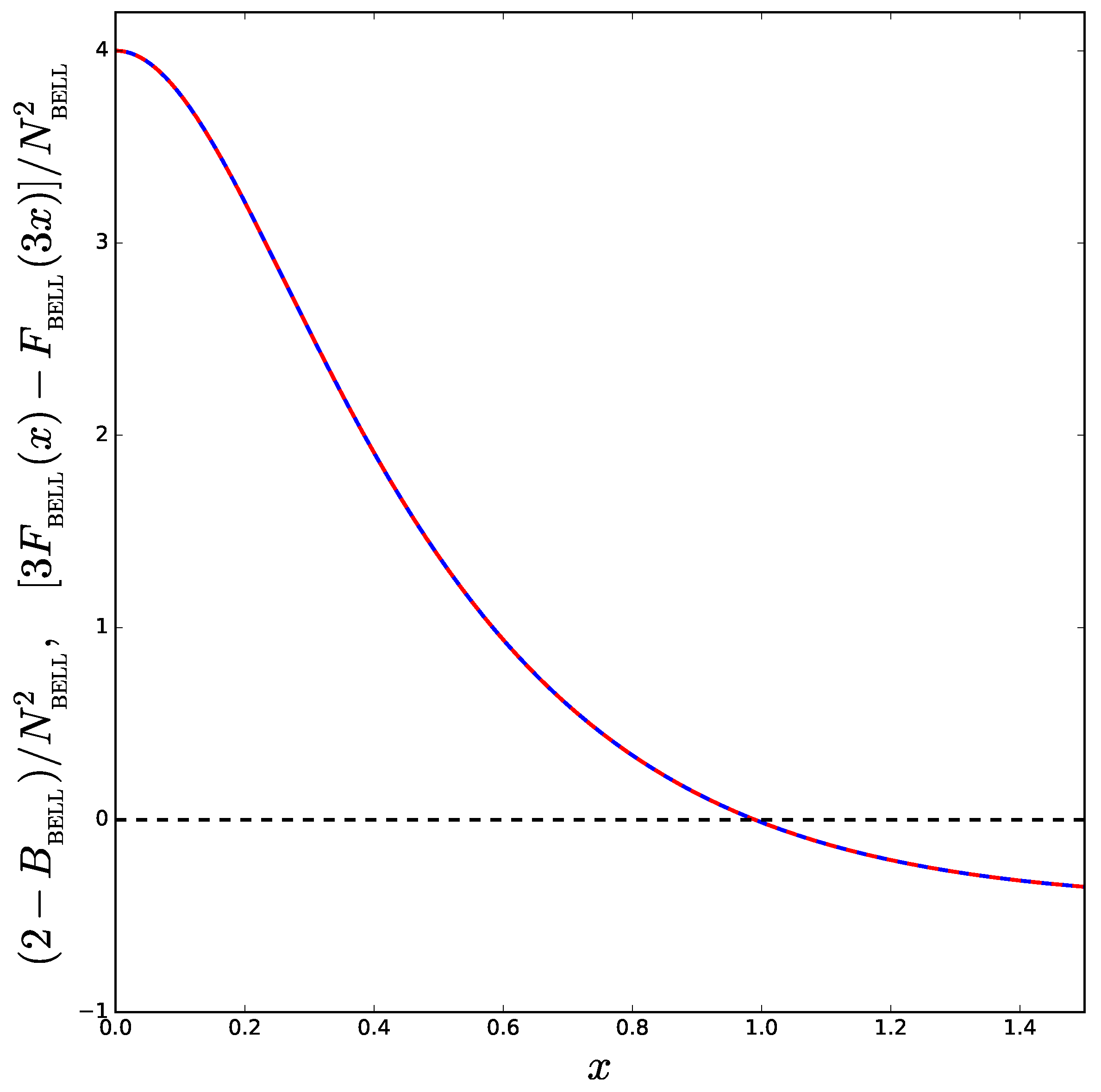
In Figure 6, we have have plotted the quantity $[2-B_{\mathrm{BELL}}(-2x,x,0,3x)]/N_{\mathrm{BELL}}^2$ (solid blue line). When this quantity is negative, the CHSH inequality is violated. We see on the plot that this is indeed the case provided $x>0.989761$, a conclusion also reached by Bell. Notice that one can obtain this result regardless of the value of $N_{\mathrm{BELL}}$. In Figure 6, we have also represented the quantity $[3F_{\mathrm{BELL}}\left(x\right)-F_{\mathrm{BELL}}\left(3x\right)]/N_{\mathrm{BELL}}^2$ (dashed red line), where $F_{\mathrm{BELL}}$ has been defined above. Evidently, according to the previous considerations, it should exactly coincide with $[2-B_{\mathrm{BELL}}(-2x,x,0,3x)]/N_{\mathrm{BELL}}^2$ and one checks that this is indeed the case. The condition $3F_{\mathrm{BELL}}\left(x\right)-F_{\mathrm{BELL}}\left(3x\right)\ge 0$ for a non violation of the CHSH inequality is Equation (25) of Bell’s paper.

Based on the previous considerations, Bell concludes that the non-positivity of the Wigner function (110) implies a violation of the CHSH inequality. He also adds that “I do not know that the failure of W to be non-negative is a sufficient condition in general for a locality paradox”. Although it is fair to say that the main message is not explicitly expressed in this way, it is however clear that Bell’s letter suggests a (one-to-one?) correspondence between a violation of the CHSH inequality and the non-positivity of the Wigner distribution. This argument seems to be supported by the EPR example (positive Wigner function and no violation of CHSH) and by the example we have just studied (no positive definite Wigner function and violation of CHSH). After all, the non-positivity of the Wigner function certainly signals that some genuine quantum effects are at play and, when this is the case, it is natural to think that Bell inequality could be violated. Therefore, at first sight, this conclusion appears to be meaningful and correct. It has very important consequences for Cosmology. Indeed, as we have already seen, cosmological perturbations are placed in a two-mode squeezed state, which is a Gaussian state, and, therefore, has a positive definite Wigner function. As a consequence, Bell’s result, if true, would imply that no violation of his inequality can be observed in the CMB.

4.4. Is Bell’s Paper Wrong?

In 1997, the article [30] was published by L. Johansen in Physics Letters A. In brief, this article claims that Bell’s paper is wrong. The main argument is that working with Equation (108), namely with a wave function ${\Psi }_{\mathrm{BELL}}(q_1,q_2)=N_{\mathrm{BELL}}\left[{\left(q_1-q_2+q_0\right)}^2-2a^2\right]e^{-{(q_1-q_2+q_0)}^2/\left(2a^2\right)}$, where $N_{\mathrm{BELL}}$ is just viewed as a constant, is incorrect because, as we have already noticed in the previous section, this wavefunction is not correctly normalized. Ref. [30] quotes the book by A. Peres, “Quantum Theory: Concepts and Methods” where, on p. 80, one is warned that not normalizing properly the wavefunction can lead to negative probabilities or to probabilities larger than one.

Then, Ref. [30] makes his argument more precise and states that Bell’s mistake is in fact to treat the normalization factor $N_{\mathrm{BELL}}$ as time independent. However, what Ref. [30] does in practice is in fact much more interesting for the question discussed here. The idea is to consider a Wigner function which is positive definite, then use Bell’s mathematical trick described above and, finally, show that this implies of violation of the CHSH inequality. Since, according to Ref. [30], one cannot have a CHSH inequality violation if the Wigner function is positive definite, it follows that Bell’s mathematical trick and, therefore, Bell’s result must be incorrect. This is a reductio ad absurdum proof. What is especially interesting is the fact that the correspondence positivity of the Wigner distribution versus impossibility to violate Bell inequality is taken for granted or is considered as obvious by the author.

Let us now study in detail the results of Ref. [30]. The starting point is the following Wigner function

$$\begin{array}{c}\hfill W_{\mathrm{J}}(q_1,q_2,p_1,p_2)=\frac{1}{{\pi }^2}{e}^{-{[(q_1-q_2)/\sqrt{2}-q_0]}^2-{[(p_1-p_2)/\sqrt{2}-p_0]}^2}{e}^{-s^2{(q_1+q_2)}^2/2-{(p_1+p_2)}^2/\left(2s^2\right)},\end{array}$$

(115)

which is obviously positive definite. In fact, this is the product of the Wigner function of a coherent state with the Wigner function of a squeezed state. One can also check that this Wigner function is correctly normalized. Then, Ref. [30] proceeds and applies Bell’s trick consisting in working with unnormalized states to the Wigner function (115). In order to see what it means in the present context, the best is to calculate the Wigner function associated with the wavefunction (109). Recall that the wavefunction (109) is the correctly normalized version of the unnormalized wavefunction (108) considered before and used by Bell to show that a non-positive Wigner function may cause a CHSH inequality violation. Assuming the wavefunction (109), the corresponding Wigner function reads

$$\begin{array}{cc}\hfill W_{\mathrm{BELL}}(q_1,q_2,p_1,p_2)& =\frac{4}{11{\pi }^3{a}^{5}b}b\sqrt{\pi }{e}^{-b^2{(p_1+p_2)}^2/4-{(q_1+q_2)}^2/b^2}\sqrt{\pi }{a}^5{e}^{-a^2{(p_1-p_2)}^2/4-{(q_1-q_2+q_0)}^2/a^2}\hfill \\ & \left\{\frac{11}{4}+{\left[\frac{{(q_1-q_2+q_0)}^2}{a^2}+\frac{a^2}{4}{(p_1-p_2)}^2\right]}^2+\frac{a^2}{4}{(p_1-p_2)}^2-5\frac{{(q_1-q_2+q_0)}^2}{a^2}\right\}.\hfill \end{array}$$

(116)

As discussed before, Bell claims that one can take the limit $b\to \infty$ from the very beginning, which consists of killing the term proportional to ${(q_1+q_2)}^2$ and boosting the term proportional to ${(p_1+p_2)}^2$ in the argument of the first exponential. In the limit $b\to \infty$, one has $b\sqrt{\pi }{e}^{-b^2{(p_1+p_2)}^2/4}\to 2\pi \delta (p_1+p_2)$ and recalling that $N_{\mathrm{BELL}}^2=8/\left(11\pi a^{5}b\right)e^{-{(q_1+q_2)}^2/b^2}$, we see that we exactly arrive at the Wigner function considered by Bell in his article, namely Equation (110) (for $a=1$, which is the choice made in Bell’s article). The conclusion is that Bell’s limit or trick is equivalent to killing the term proportional to ${(q_1+q_2)}^2$ and boosting the term $\propto {(p_1+p_2)}^2$ in the Wigner function.

Therefore, coming back to Equation (115) and to the article [30], this corresponds to taking the limit $s\to 0$, leading to

$$\begin{array}{c}\hfill W_{\mathrm{J}}(q_1,q_2,p_1,p_2)=\frac{K}{\pi }{e}^{-{[(q_1-q_2)/\sqrt{2}-q_0]}^2-{[(p_1-p_2)/\sqrt{2}-p_0]}^2}\delta (p_1+p_2),\end{array}$$

(117)

where $K=\sqrt{2/\pi }s{e}^{-s^2{(q_1+q_2)}^2/2}$. We see that this Wigner function also contains a Dirac function of $p_1+p_2$ as in Equation (110), which confirms that Bell’s limit has indeed been correctly implemented in Equation (115). As already noticed before, Ref. [30] remarks that K is what Bell calls an “an unimportant constant”. Here, we have calculated K in term of s, which is not done in Ref. [30].

Then, we repeat once more the standard procedure. We first calculate ${\rho }_{\mathrm{J}}(q_1,q_2,t_1,t_2)$ by integrating the Wigner function over $p_1$ and $p_2$. We find

$$\begin{array}{c}\hfill {\rho }_{\mathrm{J}}(q_1,q_2,t_1,t_2)=\frac{K}{\sqrt{2\pi }}\frac{1}{\sqrt{1+{\tau }^2}}{e}^{-{[(q_1-q_2)/\sqrt{2}-q_0\left(\tau \right)]}^2/(1+{\tau }^2)},\end{array}$$

(118)

where $\tau \equiv (t_1+t_2)/2$ (recall that Bell defines $\tau$ as $t_1+t_2$) and $q_0\left(\tau \right)\equiv q_0+p_0\tau$. This expression exactly coincides with Equation (10) of Ref. [30]. The only difference is that the constant K is divided by $\sqrt{\pi }$ instead of $\sqrt{2\pi }$ in the above expression. This factor $\sqrt{2}$ is just due to the fact that Ref. [30] has a slightly different definition of K: according to its Equation (3), it is indeed the overall constant for the Wigner function (117) if the Dirac function appearing is written as $\delta [(p_1+p_2)/\sqrt{2}]$, while in our case the Dirac function is simply written $\delta (p_1+p_2)$. This difference accounts for the $\sqrt{2}$ between the two expressions.

Although Ref. [30] is supposed to mimic Bell’s paper exactly, there are other differences between the two articles. One, which is only a detail, is that Ref. [30] defines the sign operators, or pseudo spin operators, with $q_0=0$, namely ${\widehat{S}}_1\left(t_1\right)=\mathrm{sgn}\left({\widehat{q}}_1,t_1\right)$ and ${\widehat{S}}_2\left(t_2\right)=\mathrm{sgn}\left({\widehat{q}}_2,t_2\right)$. However, this does not affect the discussion since it was shown before that Bell’s result does not depend on $q_0$. This also means that Equation (94) now reads $E_{\mathrm{J}}(t_1,t_2)=1-2[{\int }_0^{+\infty }\mathrm{d}{q}_1{\int }_{-\infty }^0\mathrm{d}{q}_2\rho \left(q_1,q_2,t_1,t_2\right)+{\int }_{-\infty }^0\mathrm{d}{q}_1{\int }_0^{+\infty }\mathrm{d}{q}_2\rho \left(q_1,q_2,t_1,t_2\right)]$. Inserting Equation (118) in this last expression, one finds that

$$\begin{array}{c}\hfill E_{\mathrm{J}}(t_1,t_2)=1-2\sqrt{2}K\left\{\frac{\sqrt{1+{\tau }^2}}{\sqrt{\pi }}{e}^{-q_0^2\left(\tau \right)/(1+{\tau }^2)}+q_0\left(\tau \right)\mathrm{erf}\left[\frac{q_0\left(\tau \right)}{\sqrt{1+{\tau }^2}}\right]\right\},\end{array}$$

(119)

which coincides with Equation (14) of Ref. [30] (up to the factor $\sqrt{2}$ already mentioned above). Following Bell, Ref. [30] simply defines $F_{\mathrm{J}}\left(\tau \right)$ by $E_{\mathrm{J}}(t_1,t_2)=1-F_{\mathrm{J}}\left(\tau \right)$, which means that

$$\begin{array}{c}\hfill F_{\mathrm{J}}\left(\tau \right)=2\sqrt{2}K\left\{\frac{\sqrt{1+{\tau }^2}}{\sqrt{\pi }}{e}^{-q_0^2\left(\tau \right)/(1+{\tau }^2)}+q_0\left(\tau \right)\mathrm{erf}\left[\frac{q_0\left(\tau \right)}{\sqrt{1+{\tau }^2}}\right]\right\},\end{array}$$

(120)

in agreement with Equation (14) of this paper.

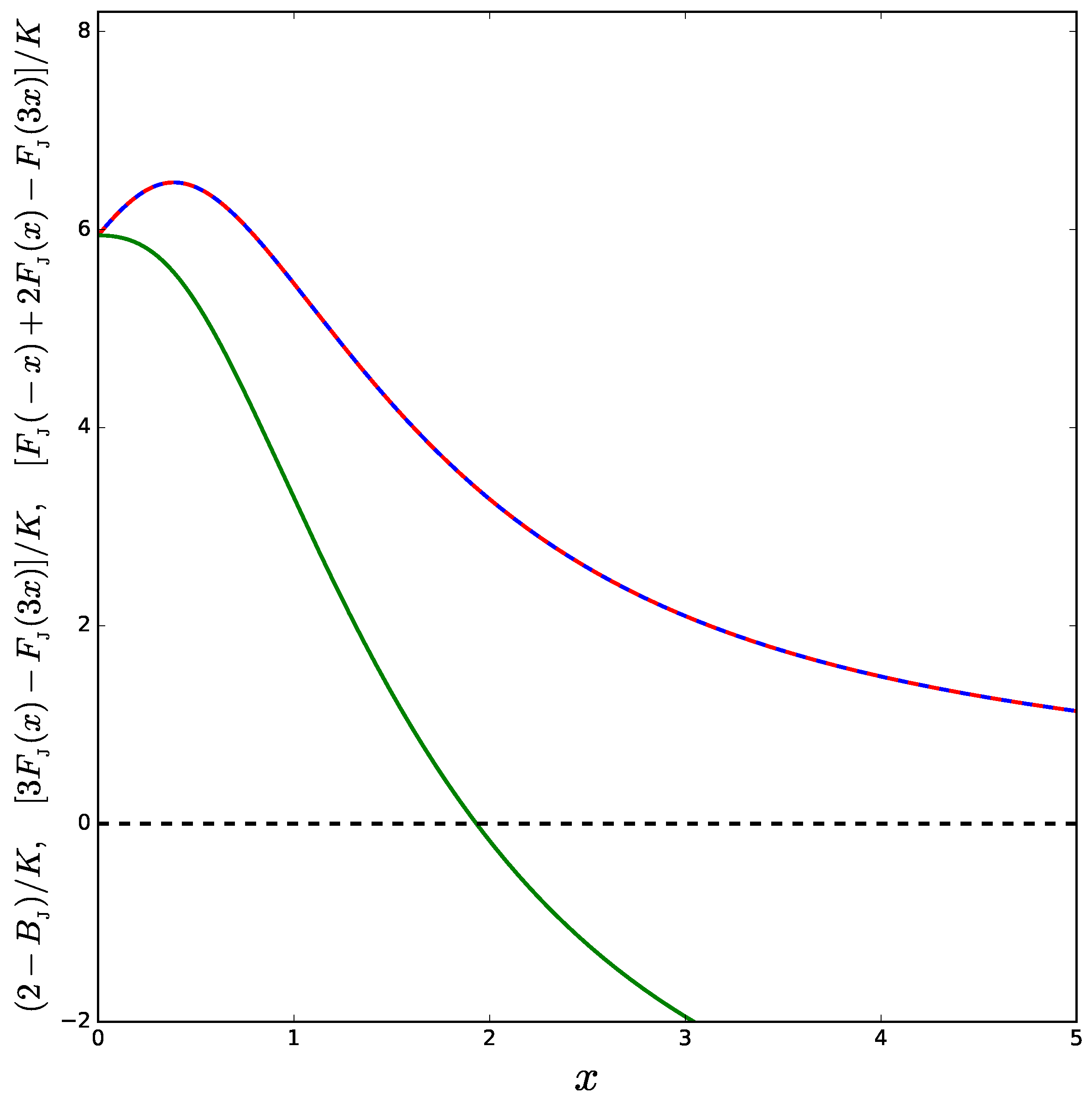
Finally, Ref. [30] computes the mean value of the Bell operator given in Equation (114), namely for $t_1=-2x$, $t_2=x$, $t_1^{\prime }=0$, $t_2^{\prime }=3x$. Following Bell, Ref. [30] studies the function $3F_{\mathrm{J}}\left(x\right)-F_{\mathrm{J}}\left(3x\right),$ which, if it takes negative values, signals a violation of the CHSH inequality—see the discussion around Equation (114). Ref. [30] notices that, if, for instance, one chooses $q_0=1$ and $p_0=-1$, this is precisely the case in the limit $x\gtrsim 1$—see Figure 1 of this article. In Figure 7, we have checked that, indeed, the function $3F_{\mathrm{J}}\left(x\right)-F_{\mathrm{J}}\left(3x\right)$ can be negative—see the green solid line. Notice that the scales in Figure 7 and in Figure 1 of Ref. [30] do not coincide because of the slight difference in the definition of $\tau$ already signaled before.

Therefore, by using Bell’s trick, Ref. [30] arrives at a violation of the CHSH inequality starting with a Wigner function which is positive definite. According to this paper, this is impossible because a positive Wigner function necessarily implies that the CHSH inequality cannot be violated. As a consequence, Ref. [30] concludes that the only way out is that Bell’s trick, and therefore his entire paper, is incorrect. The deep reason for this mistake is that “one is not allowed to assume that K is time independent”.

4.5. Are Criticisms against Bell’s Paper Wrong?

Let us now examine in more details the considerations of Ref. [30] presented in the previous section.

A first remark is that Ref. [30] has $p_0\ne 0$ while there is no $p_0$ in Bell’s article. This difference turns out to be crucial because, if Bell’s function $F_{\mathrm{BELL}}$ defined in Equation (112) only depends on ${\tau }^2$, $F_{\mathrm{J}}$ in Ref. [30] defined in Equation (119) depends on $\tau$ precisely because of the presence of $p_0$ [since $q_0\left(\tau \right)=q_0+p_0\tau$]. Only when $p_0=0$ does this become a function of ${\tau }^2$ only. This turns out to have drastic consequences. Indeed, since $F_{\mathrm{J}}(-x)\ne F_{\mathrm{J}}\left(x\right)$, one cannot say that $F_{\mathrm{J}}(-x)+2F_{\mathrm{J}}\left(x\right)-F_{\mathrm{J}}\left(3x\right)=3F_{\mathrm{J}}\left(x\right)-F_{\mathrm{J}}\left(3x\right)$ and a signature of a CHSH inequality violation is $F_{\mathrm{J}}(-x)+2F_{\mathrm{J}}\left(x\right)-F_{\mathrm{J}}\left(3x\right)\le 0$ and no longer $3F_{\mathrm{J}}\left(x\right)-F_{\mathrm{J}}\left(3x\right)\le 0$; and it turns out that if $3F_{\mathrm{J}}\left(x\right)-F_{\mathrm{J}}\left(3x\right)$ does become negative (see the solid green line in Figure 7, this is not the case for $F_{\mathrm{J}}(-x)+2F_{\mathrm{J}}\left(x\right)-F_{\mathrm{J}}\left(3x\right)$ as shown in Figure 7 (see the dashed red line). This clearly invalidates the whole reasoning of Ref. [30]: Bell’s mathematical trick has not led to a fake CHSH violation for the Wigner function (115).

Second, Ref. [30] claims that Bell’s mistake is to have ignored the time dependence of the constant K. However, the constant K was calculated before and reads $K=\sqrt{2/\pi }s{e}^{-s^2{(q_1+q_2)}^2/2}$. It does not contain any time dependence so this argument is incorrect as well.

Third, let us notice that the Wigner function considered in Ref. [30], namely Equation (115), is nothing but a special case of the EPR Wigner function (97) considered in Section 4.3. Indeed, if one takes $b=2/s$, $\epsilon =2$, $q_0\to \sqrt{2}{q}_0$, then Equation (97) becomes identical to Equation (115) with $p_0=0$. However, we have established before that, if the state of the system is the EPR state, then no CHSH violation can occur. This means that, if we had found a violation of the CHSH inequality starting from the Wigner function (115), this would have indeed indicated a mathematical inconsistency somewhere, as argued by Ref. [30]. However, this is not the case since the CHSH inequality is never violated as can be seen in Figure 7 where $(2-B_{\mathrm{J}})/K$ is represented (solid blue line) and is always positive, a conclusion already obtained before from the plot of the combination $[F_{\mathrm{J}}(-x)+2F_{\mathrm{J}}\left(x\right)-F_{\mathrm{J}}\left(3x\right)]/K$ represented by the dashed red line. Therefore, this is an additional reason why the argument of Ref. [30], which is entirely based on this belief, would have remained, in any case, problematic. We therefore conclude that the criticisms put forward in Ref. [30] against Bell’s paper are incorrect.

4.6. Correct or Not Correct?

Before closing this section, let us examine again Bell results. After all, the fact that the criticisms against them are wrong does not mean that Bell’s paper is correct. As guessed in Ref. [30], we believe that Bell’s treatment of the wavefunction normalization is problematic. We have established before that

$$\begin{array}{c}\hfill N_{\mathrm{BELL}}=\sqrt{\frac{8}{11\pi a^{5}b}}{e}^{-{(q_1+q_2)}^2/b^2}.\end{array}$$

(121)

Bell’s main idea is to ignore the dependence in $q_1+q_2$ by sending b to infinity in the argument of the exponential. However, we see in the above expression that, in fact, this sends the whole normalization factor, and therefore the whole wavefunction to zero! The same remark of course applies to the exact Wigner function calculated in Equation (116). Therefore, this procedure cannot be correct. Moreover, $N_{\mathrm{BELL}}$ is a function of $q_1$ and $q_2$ and, as a consequence, when one integrates ${\rho }_{\mathrm{BELL}}$ over ${\overline{q}}_1$ and ${\overline{q}}_2$ in Equation (112), it is simply incorrect to treat $N_{\mathrm{BELL}}$ as a constant. Therefore, we also reach the conclusion that Bell’s article is incorrect even if for completely different reasons from those put forward in Ref. [30].

4.7. Revzen’s Theorem

We are apparently in a complex situation: we have found that Bell’s paper establishing a connection between the non-positivity of the Wigner function and a CHSH inequality violation is incorrect, but we have also reached the conclusion that the criticisms expressed against that paper are wrong as well! Moreover, all these authors seem to agree that, if the Wigner function is positive definite, then no CHSH inequality violation can occur, which, we recall, would have important conceptual consequences for Cosmology.

In fact, the situation was clarified in 2004 in Refs. [60,61]. In these papers, Revzen establishes that, under certain conditions that we are going to describe, Bell inequality can be violated even if the Wigner distribution is positive definite. Notice that this both invalidates Bell’s paper [27], since Revzen’s result shows that a Bell inequality violation is not necessarily associated with a negative Wigner function, but also Ref. [30] since its reasoning was entirely based on the fact that violating Bell’s inequality is impossible if the Wigner function is positive. In his paper, Revzen mentions Bell’s paper [27] but says that “Bell’s original argument that nonnegativity of Wigner’s function suffices to preclude Bell inequality violation was shown to be inaccurate” in Ref. [30]. He adds that “Difficulties in handling normalization of the EPR state considered by Bell were shown to involve a misleading factor”. As explained in the last section, this description is not very accurate since we have just shown that the criticisms of Ref. [30] are in fact not valid.

Let us now come to the main result obtained by Revzen. In brief, Revzen shows that Bell inequality can be violated even if the Wigner function is positive definite provided the variables considered are “improper”, namely if the Weyl transform (defined in Equation (42)) of an operator takes different values than the spectrum of that operator. Let us give an example of a proper and improper operators. First, let us consider the pseudo spin operators used by Bell, namely $\widehat{S}=\mathrm{sgn}(\widehat{q},t)$. Its Weyl transform is given by

$$\begin{array}{cc}\hfill \tilde{S}& =\int \mathrm{d}x{e}^{-i\pi x}〈q+\frac{x}{2}\left|\mathrm{sgn}\left(\widehat{q}\right)\right|q-\frac{x}{2}〉=\int \mathrm{d}x{e}^{-i\pi x}\mathrm{sgn}\left(q-\frac{x}{2}\right)〈q+\frac{x}{2}|q-\frac{x}{2}〉\hfill \\ & =\int \mathrm{d}x{e}^{-i\pi x}\mathrm{sgn}\left(q-\frac{x}{2}\right)\delta \left(x\right)=\mathrm{sgn}\left(q\right).\hfill \end{array}$$

(122)

Therefore, this operator is proper since its Weyl transform takes values $\pm 1$ which are exactly the values taken by the spectrum of the operator. This explains why, in the EPR state, Bell inequality was not violated in Section 4.3. This was a situation where the Wigner function was positive and the operator used to construct the Bell operator was proper.

Let us now give an example of an improper operator. Let us consider the following operator

$$\begin{array}{c}\hfill {\widehat{s}}_z={\displaystyle \sum _{n=0}^{\infty }}\left(|2n+1\rangle \langle 2n+1|-|2n\rangle \langle 2n|\right).\end{array}$$

(123)

The reason for the notation ${\widehat{s}}_z$ will be clarified below. Here, $|n\rangle$ is an eigenvector of the number operator. It is easy to show that the spectrum of this operator is $\pm 1$ because ${\widehat{s}}_z^2=\widehat{\mathbb{I}}$. The matrix element of ${\widehat{s}}_z$ is given by $\langle m|{\widehat{s}}_z|m^{\prime }\rangle =\pm {\delta }_{m{m}^{\prime }}$ with a plus sign if m is odd and a minus sign if m is even. This allows us to rewrite ${\widehat{s}}_z$ as

$$\begin{array}{c}\hfill {\widehat{s}}_z=-{\int }_{-\infty }^{\infty }\mathrm{d}q|q\rangle \langle -q|.\end{array}$$

(124)

Indeed, one can show that this leads to the same matrix element, namely

$$\begin{array}{c}\hfill \langle m|{\widehat{s}}_z|m^{\prime }\rangle =-{\int }_{-\infty }^{+\infty }\mathrm{d}q\langle m|q\rangle \langle -q|m^{\prime }\rangle =\frac{-{(-1)}^{m^{\prime }}}{\sqrt{\pi 2^{m+m^{\prime }}m!m^{\prime }!}}{\int }_{-\infty }^{+\infty }\mathrm{d}q{H}_m\left(q\right)H_{m^{\prime }}\left(q\right)e^{-q^2}=-{(-1)}^m{\delta }_{m{m}^{\prime }},\end{array}$$

(125)

where $H_m$ is a Hermite polynomial of order n [52]. It follows that

$$\begin{array}{cc}\hfill \widetilde{s_z}& =-\int \mathrm{d}x{e}^{-i\pi x}〈q+\frac{x}{2}|\int \mathrm{d}\overline{q}\left|\overline{q}\right.〉\left.〈-\overline{q}\right|q-\frac{x}{2}〉=-\int \mathrm{d}x\int \mathrm{d}\overline{q}{e}^{-i\pi x}\delta \left(q+\frac{x}{2}-\overline{q}\right)\delta \left(-\overline{q}-q+\frac{x}{2}\right)\hfill \\ & =-\delta (-2q)\int \mathrm{d}x{e}^{-i\pi x}=-\pi \delta \left(q\right)\delta \left(\pi \right).\hfill \end{array}$$

(126)

Clearly, the Weyl transform of ${\widehat{s}}_z$ does not take values $\pm 1$ and, as a consequence, this operator is improper.

The Revzen theorem rests on Equations (43) and (44). Indeed, according to these equations, the mean value of an operator is the average of its Weyl transform weighted by the Wigner function. If the Weyl transform takes the same values as the spectrum of the operator, it means that any quantum average can be obtained through the usual, classical, laws of random variables. However, if this is so, Bell’s theorem precisely tells us that its inequality cannot be violated.

We conclude that the history of the relationship between the possibility of violating Bell inequality and the positivity of the Wigner function is a long, chaotic and rich one. For Cosmology, this question is absolutely crucial since the Wigner function is, in this case, positive definite. The Revzen theorem establishes the possibility of a Bell inequality violation in the sky, a fascinating possibility indeed. In his paper, Revzen precisely discusses his theorem with the help of a two-mode squeezed state. What was not realized before is that Cosmology provides a perfect situation to illustrate this problem. It was not realized by the cosmology community because the issues related to quantum foundations are, usually, far from its everyday interests and it was not realized by people working on Quantum Mechanics because the inflationary mechanism and the fact that cosmological perturbations are placed in a two-mode squeezed state was largely ignored by people working in this field. In fact, given that Cosmology is the part of physics where the largest squeezing is achieved, one can even argue that it is the most interesting situation to discuss the issues tackled in this section.

5. Bell Inequality Violation in the CMB?

We have just seen that, even if the CMB is placed in a quantum state with positive Wigner function, Revzen’s theorem is compatible with Bell inequality violation in the sky. Based on this result, the next question is of course to identify improper variables in the CMB that could be used for that purpose. In fact, it turns out that it is possible to build improper pseudo spin operators out of a continuous variable, here of course taken to be the Fourier amplitude of curvature perturbations. A first example has been considered by Banaszek and Wodkiewics (BM) in Ref. [56] and Chen, Pan, Hou and Zhang in Ref. [57]. They have defined the following operators:

$$\begin{array}{ccc}\hfill {\widehat{s}}_x\left(\mathit{k}\right)& =& {\displaystyle \sum _{n=0}^{\infty }}\left(|2n_{\mathit{k}}+1\rangle \langle 2n_{\mathit{k}}|+|2n_{\mathit{k}}\rangle \langle 2n_{\mathit{k}}+1|\right),\hfill \end{array}$$

(127)

$$\begin{array}{ccc}\hfill {\widehat{s}}_y\left(\mathit{k}\right)& =& i{\displaystyle \sum _{n=0}^{\infty }}\left(|2n_{\mathit{k}}\rangle \langle 2n_{\mathit{k}}+1|-|2n_{\mathit{k}}+1\rangle \langle 2n_{\mathit{k}}|\right),\hfill \end{array}$$

(128)

$$\begin{array}{ccc}\hfill {\widehat{s}}_z\left(\mathit{k}\right)& =& {\displaystyle \sum _{n=0}^{\infty }}\left(|2n_{\mathit{k}}+1\rangle \langle 2n_{\mathit{k}}+1|-|2n_{\mathit{k}}\rangle \langle 2n_{\mathit{k}}|\right),\hfill \end{array}$$

(129)

where $|n_{\mathit{k}}\rangle$ are the eigenvectors of the particle number operator. These operators are spin operators because they satisfy $\left[{\widehat{s}}_x,{\widehat{s}}_y\right]=2i{\widehat{s}}_z$, $\left[{\widehat{s}}_x,{\widehat{s}}_z\right]=-2i{\widehat{s}}_y$ and $\left[{\widehat{s}}_y,{\widehat{s}}_z\right]=2i{\widehat{s}}_x$ and that their spectrum is $\pm 1$. Notice that the z-component is precisely the state we discussed in Equation (123).

Another example of fictitious spin operators are those introduced by Gour, Khanna, Mann and Revzen (GKMR) in Ref. [58], which are given by

$$\begin{array}{cc}\hfill {\widehat{\mathcal{S}}}_x& ={\int }_0^{+\infty }\mathrm{d}{q}_{\mathit{k}}\left(|{\mathcal{E}}_{\mathit{k}}\rangle \langle {\mathcal{O}}_{\mathit{k}}|+|{\mathcal{O}}_{\mathit{k}}\rangle \langle {\mathcal{E}}_{\mathit{k}}|\right),\hfill \end{array}$$

(130)

$$\begin{array}{cc}\hfill {\widehat{\mathcal{S}}}_y& =i{\int }_0^{+\infty }\mathrm{d}{q}_{\mathit{k}}\left(|{\mathcal{O}}_{\mathit{k}}\rangle \langle {\mathcal{E}}_{\mathit{k}}|-|{\mathcal{E}}_{\mathit{k}}\rangle \langle {\mathcal{O}}_{\mathit{k}}|\right),\hfill \end{array}$$

(131)

$$\begin{array}{cc}\hfill {\widehat{\mathcal{S}}}_z& =-{\int }_0^{+\infty }\mathrm{d}{q}_{\mathit{k}}\left(|{\mathcal{E}}_{\mathit{k}}\rangle \langle {\mathcal{E}}_{\mathit{k}}|-|{\mathcal{O}}_{\mathit{k}}\rangle \langle {\mathcal{O}}_{\mathit{k}}|\right),\hfill \end{array}$$

(132)

where $|{\mathcal{E}}_{\mathit{k}}\rangle$ and $|{\mathcal{O}}_{\mathit{k}}\rangle$ are defined by

$$\begin{array}{cc}\hfill |{\mathcal{E}}_{\mathit{k}}\rangle & =\frac{1}{\sqrt{2}}\left(|q_{\mathit{k}}\rangle +|-q_{\mathit{k}}\rangle \right),|{\mathcal{O}}_{\mathit{k}}\rangle =\frac{1}{\sqrt{2}}\left(|q_{\mathit{k}}\rangle -|-q_{\mathit{k}}\rangle \right).\hfill \end{array}$$

(133)

Here, $|q_{\mathit{k}}\rangle$ is an eigenstate of the position operator for the mode $\mathit{k}$. Let us notice that, in principle, it is not an eigenstate of curvature perturbations—see also Equation (137) below.

There exists a third way to define fictitious spin operators as shown by Larsson in Ref. [62]. The z-component of the Larsson spin operators can be defined as

$$\begin{array}{cc}\hfill {\widehat{S}}_z(\ell )& ={\displaystyle \sum _{n=-\infty }^{\infty }}{(-1)}^n{\int }_{n\ell }^{(n+1)\ell }\mathrm{d}{q}_{\mathit{k}}|q_{\mathit{k}}\rangle \langle q_{\mathit{k}}|,\hfill \end{array}$$

(134)

where ℓ is a free parameter that can be arbitrarily chosen. The other components can then be introduced once the step operator

$$\begin{array}{c}\hfill {\widehat{S}}_{+}(\ell )={\displaystyle \sum _{n=-\infty }^{\infty }}{\int }_{2n\ell }^{(2n+1)\ell }\mathrm{d}{q}_{\mathit{k}}\left|q_{\mathit{k}}\rangle \langle q_{\mathit{k}}+\ell \right|\end{array}$$

(135)

has been defined and ${\widehat{S}}_{-}(\ell )={\widehat{S}}_{+}^{†}(\ell )$. They are given by ${\widehat{S}}_x(\ell )={\widehat{S}}_{+}(\ell )+{\widehat{S}}_{-}(\ell )$, ${\widehat{S}}_y(\ell )=-i\left[{\widehat{S}}_{+}(\ell )-{\widehat{S}}_{-}(\ell )\right]$.

It can be checked that, among each set of fictitious spin operators, there are at least two spin components that are improper operators [24,25,26]. As discussed before, this implies that, despite the positivity of the Wigner function, they can be used to define a quantity that violates Bell inequality. What should be done is just to follow the pioneering ideas of Bell’s paper and implement Bell inequality with the pseudo spin operators in its CHSH version.

In practice, this is done as follows. First, we view the CMB has a bipartite system made of two sub-systems corresponding to mode $\mathit{k}$ and $-\mathit{k}$. Second, we calculate the following quantity

$$\begin{array}{c}\hfill \langle {\Psi }_{2\mathrm{sq}}|\widehat{\mathcal{B}}\left(\mathit{k},-\mathit{k}\right)|{\Psi }_{2\mathrm{sq}}\rangle =E\left({\theta }_n,{\theta }_m\right)+E\left({\theta }_n,{\theta }_{m^{\prime }}\right)+E\left({\theta }_{n^{\prime }},{\theta }_m\right)-E\left({\theta }_{n^{\prime }},{\theta }_{m^{\prime }}\right),\end{array}$$

(136)

where the two-point correlation function $E(\mathit{n},\mathit{m})$ is defined by $E(\mathit{n},\mathit{m})=\langle {\Psi }_{2\mathrm{sq}}|\mathit{n}·\widehat{\mathfrak{S}}\left(\mathit{k}\right)\otimes \mathit{m}·\widehat{\mathfrak{S}}\left(-\mathit{k}\right)|{\Psi }_{2\mathrm{sq}}\rangle$, $\widehat{\mathfrak{S}}$ denoting a spin operator of one of the three types introduced before. The vector $\mathit{n}$ is a unit vector that can be written as $\mathit{n}=\left(sin{\theta }_{n}cos{\phi }_n,sin{\theta }_{n}sin{\phi }_n,cos{\theta }_n\right)$ (in the following, we choose vanishing azimuthal angles). We have calculated the mean of the Bell operator for the three sets of pseudo spin operators introduced before, see Refs. [25,26], and the result is displayed in Figure 8. For each of them, we find that Bell inequality can be violated (and, as a consistency check, we find that $|\langle {\Psi }_{2\mathrm{sq}}|\widehat{\mathcal{B}}\left(\mathit{k},-\mathit{k}\right)|{\Psi }_{2\mathrm{sq}}\rangle |<2\sqrt{2}$, the Cirel’Son bound [63]).

6. Discussion

Let us recap what has been achieved. According to inflation, curvature perturbations that source CMB anisotropies are placed in a two-mode squeezed state. This state has a positive Wigner function, but, nevertheless, is highly non-classical. One way to highlight this non-classical nature is by studying the Bell inequality. It turns out that, from the curvature perturbation, which is a continuous variable, one can extract dichotomic spin operators (following Bell’s paper), which allows us to study the Bell inequality in its CHSH incarnation. We have checked that, if the system is placed in a two mode squeezed state, then this inequality is indeed violated. Observing this violation would be the definitive proof that CMB anisotropies are of quantum mechanical origin. Is it possible in practice?

The first question is what it means to “measure” the spin operators. Concretely, we measure the temperature anisotropy. However, through the so-called Sachs–Wolfe effect, $\delta T/T$ is in fact a direct measurement of curvature perturbation, as explained in Equation (4). The definition of the spin operators introduced before, however, involves ${\widehat{q}}_{\mathit{k}}$ and not ${\widehat{\zeta }}_{\mathit{k}}$. These two quantities are related by

$$\begin{array}{c}\hfill {\widehat{q}}_{\mathit{k}}=\frac{z}{2}\left({\widehat{\zeta }}_{\mathit{k}}+{\widehat{\zeta }}_{-\mathit{k}}\right)+\frac{z}{2k}\left({\widehat{\zeta }}_{\mathit{k}}^{\prime }-{\widehat{\zeta }}_{-\mathit{k}}^{\prime }\right).\end{array}$$

(137)

We see that the knowledge of ${\widehat{\zeta }}_{\mathit{k}}$ is not sufficient to infer ${\widehat{q}}_{\mathit{k}}$. However, the amplitude of ${\widehat{\zeta }}_{\mathit{k}}^{\prime }$ is in fact related to the decaying mode as was established before in Equation (7). Since the curvature perturbation is conserved on large scale, this decaying mode is in fact negligible. If one accepts this reasoning, then a measurement of ${\widehat{\zeta }}_{\mathit{k}}$ is equivalent to a measurement of ${\widehat{q}}_{\mathit{k}}$.

The next question is whether this allows us to measure the spin operators? Let us discuss this question for the GKMR operators defined in Equations (130)–(132) (the same conclusion applies to the two other sets). It is interesting to notice that

$$\begin{array}{c}\hfill 〈q_{\mathit{k}}\left|\left[{\widehat{\mathcal{S}}}_x\left(\mathit{k}\right),{\widehat{q}}_{\mathit{k}}\right]\right|q_{\mathit{k}}^{\prime }〉=0,\end{array}$$

(138)

which means that ${\widehat{\mathcal{S}}}_x\left(\mathit{k}\right)$ can be, in principle, inferred from a measurement of ${\widehat{q}}_{\mathit{k}}$. However, for ${\widehat{\mathcal{S}}}_y$, one has

$$\begin{array}{cc}\hfill \langle q_{\mathit{k}}\left|\left[{\widehat{\mathcal{S}}}_y\left(\mathit{k}\right),{\widehat{q}}_{\mathit{k}}\right]\right|q_{\mathit{k}}^{\prime }\rangle & =\left(q_{\mathit{k}}-q_{\mathit{k}}^{\prime }\right)\langle -q_{\mathit{k}}|q_{\mathit{k}}^{\prime }\rangle +q_{\mathit{k}}^{\prime }\langle q_{\mathit{k}}|-q_{\mathit{k}}^{\prime }\rangle +q_{\mathit{k}}\langle q_{\mathit{k}}|q_{\mathit{k}}^{\prime }\rangle \hfill \\ & =q_{\mathit{k}}\left[\delta \left(q_{\mathit{k}}+q_{\mathit{k}}^{\prime }\right)+\delta \left(q_{\mathit{k}}-q_{\mathit{k}}^{\prime }\right)\right]\ne 0.\hfill \end{array}$$

(139)

This means that measuring ${\widehat{q}}_{\mathit{k}}$ is not sufficient to measure the y-component. This implies that we would need to measure another non commuting operator that can only be ${\widehat{\zeta }}_{\mathit{k}}^{\prime }$. There are two problems with this idea. First, we would need to measure the system again and it is not clear what it means when what is measured is the Universe itself! Maybe, by applying some ergodic reasoning, this would mean measuring different horizon patch on the last scattering surface? However, even if we succeed in doing so, measuring the derivative of curvature perturbation means measuring the decaying mode. Although it is a priori possible in principle, it practices it is clearly impossible. Recall that its amplitude is typically of the order $e^{-50}$, which seems out of reach for ever.

7. Conclusions

Let us now present our conclusions. In this article, we have studied the quantum mechanical aspects of inflationary perturbations. According to inflation, CMB anisotropies and large scale structures are nothing but quantum fluctuations amplified by gravitational instability and stretched to cosmological scales by the cosmic expansion. This raises two questions: first, data analysis in Cosmology is usually done without any reference to the quantum origin of the perturbations since these ones look classical to us. Then, how can we understand this quantum-to-classical transition? Second, if the perturbations are really of quantum-mechanical origin, is there a signature of this origin left over somewhere in the cosmological data?

It seems fair to acknowledge the frustrating aspect of the results established above. We have shown that the quantum mechanical origin of the perturbations is still encoded in the CMB map which, in some sense, contains many Schrödinger cats, a fascinating conclusion indeed! However, highlighting this signature essentially appears to be impossible in practice due to the smallness of the signal. We have therefore to find another method to check the quantum origin of the galaxies. A suggestion recently made in Ref. [24] is to use Leggett–Garg inequality rather than Bell inequality since the former one only requires the measurement of a single spin component. The price to pay, however, is that it should be done at different times, that is to say, at different redshifts. Maybe a future experiment such as Euclid [64] could be useful for that purpose since it plans to perform a “tomography” of the power spectrum. The quest continues!

To address these tricky questions, we have also shown that the ideas and questions that John Bell discusses in his letter “EPR correlations and EPW distributions”, despite the technical problems of his paper, are crucial to investigate these issues. They allow us to better understand the quantum-to-classical transition of the fluctuations and they help us to imagine what could be an unambiguous signature of their origin.

The contribution of John Bell to Cosmology is usually summarized by his letter “Quantum mechanics for cosmologists” (this is chapter 15 of the book “Speakable and unspeakable in quantum mechanics”) where he emphasizes that the interpretational issues of Quantum Mechanics are exacerbated in the context of Cosmology—see the famous quote “Was the world wavefunction waiting to jump for thousands of millions of years until a single-celled living creature appeared? Or did it have to wait a little longer for some more highly qualified measurer—with a Ph.D.?”. Here, we have argued that the article “EPR correlations and EPW distributions” is another, unrecognized, Bell’s contribution to Cosmology and to the theory of inflation which is probably even more important than “Quantum mechanics for cosmologists”. The intriguing point is that Bell’s contribution was written before the cosmology community, thanks to Grishchuk and Sidorov, realized that the inflationary perturbations are placed in a two-mode squeezed state, namely an entangled state with positive definite Wigner function.

Once more, John Bell has been a precursor!

References

- Starobinsky, A.A. A new type of isotropic cosmological models without singularity. Phys. Lett. 1980, B91, 99–102. [Google Scholar] [CrossRef]
- Starobinsky, A.A. Dynamics of phase transition in the new inflationary universe scenario and generation of perturbations. Phys. Lett. 1982, B117, 175–178. [Google Scholar] [CrossRef]
- Guth, A.H. Inflationary universe: A possible solution to the horizon and flatness problems. Phys. Rev. 1981, D23, 347. [Google Scholar] [CrossRef]
- Linde, A.D. A new inflationary universe scenario: A possible solution of the horizon, flatness, homogeneity, isotropy and primordial monopole problems. Phys. Lett. 1982, B108, 389–393. [Google Scholar] [CrossRef]
- Albrecht, A.; Steinhardt, P.J. Cosmology for grand unified theories with radiatively induced symmetry breaking. Phys. Rev. Lett. 1982, 48, 1220. [Google Scholar] [CrossRef]
- Linde, A.D. Chaotic inflation. Phys. Lett. 1983, B129, 177–181. [Google Scholar] [CrossRef]
- Chowdhury, D.; Martin, J.; Ringeval, C.; Vennin, V. Inflation after Planck: Judgment Day. arXiv, 2019; arXiv:1902.03951. [Google Scholar]
- Martin, J. Cosmic Inflation: Trick or Treat? arXiv, 2019; arXiv:1902.05286. [Google Scholar]
- Starobinsky, A.A. Spectrum of relict gravitational radiation and the early state of the universe. JETP Lett. 1979, 30, 682–685. [Google Scholar]
- Mukhanov, V.F.; Chibisov, G. Quantum fluctuations and a nonsingular universe. JETP Lett. 1981, 33, 532–535. [Google Scholar]
- Mukhanov, V.F.; Chibisov, G. Vacuum energy and large-scale structure of the universe. Sov. Phys. JETP 1982, 56, 258–265. [Google Scholar]
- Guth, A.H.; Pi, S. Fluctuations in the new inflationary universe. Phys. Rev. Lett. 1982, 49, 1110. [Google Scholar] [CrossRef]
- Hawking, S. The development of irregularities in a single bubble inflationary universe. Phys. Lett. 1982, B115, 295–297. [Google Scholar] [CrossRef]
- Bardeen, J.M.; Steinhardt, P.J.; Turner, M.S. Spontaneous creation of almost scale-free density perturbations in an inflationary universe. Phys. Rev. 1983, D28, 679. [Google Scholar] [CrossRef]
- Martin, J. Inflationary cosmological perturbations of quantum-mechanical origin. Lect. Notes Phys. 2005, 669, 199. [Google Scholar]
- Martin, J. Inflationary perturbations: The cosmological Schwinger effect. Lect. Notes Phys. 2008, 738, 193. [Google Scholar]
- Ade, P.A.R.; Aghanim, N.; Arnaud, M.; Ashdown, M.; Aumont, J.; Baccigalupi, C.; Banday, A.J.; Barreiro, R.B.; Bartlett, J.G.; Bartolo, N.; et al. Planck 2015 results-XIII. Cosmological parameters. Astron. Astrophys. 2016, 594, A13. [Google Scholar]
- Ade, P.A.R.; Aghanim, N.; Arnaud, M.; Arroja, F.; Ashdown, M.; Aumont, J.; Baccigalupi, C.; Ballardini, M.; Banday, A.J.; Barreiro, R.B.; et al. Planck 2015 results-XX. Constraints on inflation. Astron. Astrophys. 2016, 594, A20. [Google Scholar]
- Ade, P.A.R.; Aghanim, N.; Arnaud, M.; Arroja, F.; Ashdown, M.; Aumont, J.; Baccigalupi, C.; Ballardini, M.; Banday, A.J.; Barreiro, R.B.; et al. Planck 2015 results-XVII. Constraints on primordial non-Gaussianity. Astron. Astrophys. 2016, 594, A17. [Google Scholar]
- Aghanim, N.; Akrami, Y.; Ashdown, M.; Aumont, J.; Baccigalupi, C.; Ballardini, M.; Banday, A.J.; Barreiro, R.B.; Bartolo, N.; Basak, S.; et al. Planck 2018 results. VI. Cosmological parameters. arXiv, 2018; arXiv:1807.06209. [Google Scholar]
- Aghanim, Y.; Arroja, F.; Ashdown, M.; Aumont, J.; Baccigalupi, C.; Ballardini, M.; Banday, A.J.; Barreiro, R.B.; Bartolo, N.; Basak, S.; et al. Planck 2018 results. X. Constraints on inflation. arXiv, 2018; arXiv:1807.06211. [Google Scholar]
- Martin, J.; Vennin, V.; Peter, P. Cosmological inflation and the quantum measurement problem. Phys. Rev. 2012, D86, 103524. [Google Scholar] [CrossRef]
- Martin, J.; Vennin, V. Quantum discord of cosmic inflation: Can we show that CMB anisotropies are of quantum-mechanical origin? Phys. Rev. 2016, D93, 023505. [Google Scholar] [CrossRef]
- Martin, J.; Vennin, V. Leggett-Garg inequalities for squeezed states. Phys. Rev. 2016, A94, 052135. [Google Scholar] [CrossRef]
- Martin, J.; Vennin, V. Bell inequalities for continuous-variable systems in generic squeezed states. Phys. Rev. 2016, A93, 062117. [Google Scholar] [CrossRef]
- Martin, J.; Vennin, V. Obstructions to Bell CMB experiments. Phys. Rev. 2017, D96, 063501. [Google Scholar] [CrossRef]
- Bell, J.S. EPR Correlations and EPW Distributions. Ann. N. Y. Acad. Sci. 1986, 480, 263. [Google Scholar] [CrossRef]
- Bell, J.S. Speakable and Unspeakable in Quantum Mechanics. Collected Papers on Quantum Philosophy; Cambridge University Press: Cambridge, UK, 1987. [Google Scholar]
- Grishchuk, L.; Sidorov, Y. Squeezed quantum states of relic gravitons and primordial density fluctuations. Phys. Rev. 1990, D42, 3413. [Google Scholar] [CrossRef]
- Johansen, L.M. EPR correlations and EPW distributions revisited. Phys. Lett. 1997, A236, 173–176. [Google Scholar] [CrossRef]
- Peter, P.; Uzan, J.P. Primordial Cosmology; Oxford University Press: Oxford, UK, 2013. [Google Scholar]
- Mukhanov, V.F.; Feldman, H.; Brandenberger, R.H. Theory of cosmological perturbations. Phys. Rept. 1992, 215, 203–333. [Google Scholar] [CrossRef]
- Bennett, C.L.; Halpern, M.; Hinshaw, G.; Jarosik, N.; Kogut, A.; Limon, M.; Meyer, S.S.; Page, L.; Spergel, D.N.; Tucker, G.S.; et al. First-Year Wilkinson Microwave Anisotropy Probe (WMAP)* Observations: Preliminary Maps and Basic Results. Astrophys. J. Suppl. 2003, 148, 1. [Google Scholar] [CrossRef]
- Sachs, R.K.; Wolfe, A.M. Perturbations of a cosmological model and angular variations of the microwave background. Astrophys. J. 1967, 147, 73. [Google Scholar] [CrossRef]
- Seljak, U.; Zaldarriaga, M. A Line of Sight Approach to Cosmic Microwave Background Anisotropies. Astrophys. J. 1996, 469, 437–444. [Google Scholar] [CrossRef]
- Schwinger, J.S. On gauge invariance and vacuum polarization. Phys. Rev. 1951, 82, 664. [Google Scholar] [CrossRef]
- Lvovsky, A.I. Squeezed light. arXiv, 2014; arXiv:1401.4118. [Google Scholar]
- Schnabel, R. Squeezed states of light and their applications in laser interferometers. Phys. Rept. 2017, 684, 1–51. [Google Scholar] [CrossRef]
- Vahlbruch, H.; Mehmet, M.; Chelkowski, S.; Hage, B.; Franzen, A.; Lastzka, N.; Goßler, S.; Danzmann, K.; Schnabel, R. Observation of Squeezed Light with 10-dB Quantum-Noise Reduction. Phys. Rev. Lett. 2008, 100, 033602. [Google Scholar] [CrossRef]
- Vahlbruch, H.; Mehmet, M.; Danzmann, K.; Schnabel, R. Detection of 15 dB Squeezed States of Light and their Application for the Absolute Calibration of Photoelectric Quantum Efficiency. Phys. Rev. Lett. 2016, 117, 110801. [Google Scholar] [CrossRef]
- Hudson, R. When is the wigner quasi-probability density non-negative? Rep. Math. Phys. 1974, 6, 249. Available online: http://www.sciencedirect.com/science/article/pii/003448777490007X (accessed on 10 April 2019). [CrossRef]
- Hall, B. Quantum Theory for Mathematicians; Springer: New York, NY, USA, 2013; ISBN 9781461471165. Available online: https://books.google.fr/books?id=bYJDAAAAQBAJ (accessed on 10 April 2019).
- Einstein, A.; Podolsky, B.; Rosen, N. Can Quantum-Mechanical Description of Physical Reality Be Considered Complete? Phys. Rev. 1935, 47, 777. [Google Scholar] [CrossRef]
- Ollivier, H.; Zurek, W.H. Quantum discord: A measure of the quantumness of correlations. Phys. Rev. Lett. 2001, 88, 017901. [Google Scholar] [CrossRef] [PubMed]
- Henderson, L.; Vedral, V. Classical, quantum and total correlations. J. Phys. A Math. Gen. 2001, 34, 6899. [Google Scholar] [CrossRef]
- Kullback, S.; Leibler, R.A. On Information and Sufficiency. Ann. Math. Stat. 1951, 22, 79–86. [Google Scholar] [CrossRef]
- Kenfack, A.; Zyczkowski, K. Negativity of the Wigner function as an indicator of non-classicality. J. Opt. B Quantum Semiclass. Opt. 2004, 6, 396. [Google Scholar] [CrossRef]
- Berry, M.V. Semi-classical mechanics in phase space: A study of Wigner’s function. Philos. Trans. R. Soc. Lond. A 1977, A287, 237–271. [Google Scholar] [CrossRef]
- Halliwell, J.J. Correlations in the wave function of the universe. Phys. Rev. 1987, D36, 3626. [Google Scholar] [CrossRef]
- Habib, S. Classical limit in quantum cosmology: Quantum mechanics and the Wigner function. Phys. Rev. 1990, D42, 2566. [Google Scholar] [CrossRef]
- Anderson, A. On predicting correlations from Wigner functions. Phys. Rev. 1990, D42, 585. [Google Scholar] [CrossRef]
- Abramowitz, M.; Stegun, I.A. (Eds.) Handbook of Mathematical Functions with Formulas, Graphs, and Mathematical Tables, 10th ed.; U.S. Government Printing Office: Washington, DC, USA, 1972.
- Albrecht, A.; Ferreira, P.; Joyce, M.; Prokopec, T. Inflation and squeezed quantum states. Phys. Rev. 1994, D50, 4807. [Google Scholar] [CrossRef]
- Barnett, S.; Radmore, P. Methods in Theoretical Quantum Optics; Oxford Series in Optical and Imaging Sciences; Clarendon Press: Oxford, UK, 2002; ISBN 9780198563617. [Google Scholar]
- Clauser, J.F.; Horne, M.A.; Shimony, A.; Holt, R.A. Proposed Experiment to Test Local Hidden Variable Theories. Phys. Rev. Lett. 1970, 24, 549. [Google Scholar] [CrossRef]
- Banaszek, K.; Wódkiewicz, K. Testing Quantum Nonlocality in Phase Space. Phys. Rev. Lett. 1999, 82, 2009. [Google Scholar] [CrossRef]
- Chen, Z.-B.; Pan, J.-W.; Hou, G.; Zhang, Y.-D. Maximal violation of Bell’s inequalities for continuous variable systems. Phys. Rev. Lett. 2002, 88, 040406. [Google Scholar] [CrossRef] [PubMed]
- Gour, G.; Khanna, F.C.; Mann, A.; Revzen, M. Optimization of Bell’s inequality violation for continuous variable systems. Phys. Lett. A 2004, 324, 415–419. [Google Scholar] [CrossRef]
- Maudlin, T. What bell did. J. Phys. 2014, A47, 424010. [Google Scholar] [CrossRef]
- Revzen, M.; Mello, P.A.; Mann, A.; Johansen, L.M. Bell’s inequality violation with non-negative Wigner functions. Phys. Rev. 2005, A71, 022103. [Google Scholar] [CrossRef]
- Revzen, M. The Wigner Function as Distribution Function. Found. Phys. 2006, 36, 546–562. [Google Scholar] [CrossRef]
- Larsson, J.-Å. Bell inequalities for position measurements. Phys. Rev. 2004, A70, 022102. [Google Scholar] [CrossRef]
- Cirel’Son, B.S. Quantum generalizations of Bell’s inequality. Lett. Math. Phys. 1980, 4, 93–100. [Google Scholar] [CrossRef]
- Laureijs, R.; Amiaux, J.; Arduini, S.; Auguères, J.-L.; Brinchmann, J.; Cole, R.; Cropper, M.; Dabin, C.; Duvet, L.; Ealet, A.; et al. Euclid Definition Study Report. arXiv, 2011; arXiv:1110.3193. [Google Scholar]