The ATLAS Fast TracKer—Architecture, Status and High-Level Data Quality Monitoring Framework ^†

Abstract

The Fast Tracker (FTK) is a highly parallel processor dedicated to a quick and efficient reconstruction of tracks in the Pixel and Semiconductor Tracker (SCT) detectors of the ATLAS experiment at LHC. It is designed to identify charged particle tracks with transverse momentum above 1 GeV and reconstruct their parameters at an event rate of up to 100 kHz. The average latency of the processing is below 100 μs at the expected collision intensities. This performance is achieved by using custom ASIC chips with associative memory for pattern matching, while modern FPGAs calculate the track parameters. This paper describes the architecture, the current status and a High-Level Data Quality Monitoring framework of the FTK system. This monitoring framework provides an online comparison of the FTK hardware output with the FTK functional simulation, which is run on the pixel and SCT detector data at a low rate, allowing the detection of non-expected outputs of the FTK system.

1. Introduction

ATLAS [1] is one of the two general-purpose detectors of the Large Hadron Collider (LHC), built for precision tests of the Standard Model (SM), as well as searching for physics beyond the SM at TeV energy scales. Since the LHC start up, ATLAS has produced many physics results, with the big highlight being the discovery of the Higgs boson [2].

To increase the number of interesting events produced in proton-proton (p-p) collisions per unit time, the LHC increases the instantaneous luminosity of the colliding beams, yielding an ever increasing number of p-p interactions in the same bunch crossing. Therefore, along with the p-p interaction of interest, additional p-p interactions (pile-up) are practically coincident in time for the detector. In 2015, the LHC started colliding protons at a centre-of-mass energy of 13 TeV and, as shown in Figure 1a, the delivered integrated luminosity per year rose from around 4 fb${}^{-1}$ in 2015 to around 65 fb${}^{-1}$ in 2018. As a consequence of the increased instantaneous luminosity, there is a growth in the number of multiple proton-proton interactions per bunch crossing, as shown in Figure 1b, which makes the distinction between signal and background difficult and reduces the resolution of the detector. In 2015 the average number of pile-up events was ∼13 while in 2018, it reached ∼37. From 2021 to 2023, during Run III of the LHC, there will be a further increase in the luminosity as well as in the average number of pile-up events, which are estimated to be approximately 1.5 times larger with respect to the previous run. In these environments, the effective selection of interesting physics events by the ATLAS trigger system will be a big challenge.

2. The ATLAS Fast Tracker

To reduce the huge flow of data for permanent storage, the ATLAS Trigger and Data Acquisition System (Figure 2) selects events with characteristics that make them interesting for physics analyses. For this purpose, a two-stage system is used. At the first stage, custom hardware called Level-1 Trigger (L1) [4] checks the information from the calorimeters and the muon system and reduces the event rate from 40 MHz to 100 kHz. If the event is interesting, the L1 system sends an acceptance signal to all Front-End (FE) electronics, resulting in the relevant data being pushed via the Read-Out Drivers (ROD) to the Read-Out System (ROS) where they are buffered. At the second stage, the High-Level Trigger (HLT) [5] pulls data on-demand from these buffers in order to complete the online selection. The HLT is implemented as a farm of commodity PCs. The processing starts from the “Regions of Interest” (ROIs) in the event, as they are identified by the L1 trigger. The HLT uses the information from all sub-detectors in their full granularity, including the Inner Detector [6] (Insertable B-layer [7], Pixel Detector, Semiconductor Tracker, Transition Radiation Tracker). Adding the track information in the trigger decision can significantly improve the efficiency for retaining interesting physics signals (e.g., $H\to \tau \tau$ or $H\to b\overline{b}$ events), while at the same time gives more handles to reject background. However, as the instantaneous luminosity increases, the higher detector occupancies makes the task of track reconstruction more difficult, requiring longer times to complete. Thus, while the HLT needs to employ significantly more sophisticated algorithms to deal with these conditions, it is left with potentially little time to execute them. To remove this burden from the HLT, a dedicated hardware system, called the Fast TracKer [8] (FTK) recognizes and reconstructs all tracks with transverse momentum ($p_T$) above 1 GeV and provides them to the HLT before it starts processing the event.

The FTK uses the hits of the twelve silicon layers of the Inner Detector to calculate the track parameters. A “Hit”, as used here, refers to the cluster centroid of the particle’s energy deposition, as it traverses a silicon layer. The track information is written into dedicated buffers in the Read Out System (ROS), where it is kept until requested for by the HLT. Upon the acceptance of the event, the full information produced so far (i.e., full-granularity detector information, as well as the information produced by the Trigger system, including the FTK) is built into a complete “event”, which is written to local disks by the System Farm Output. These events are then shipped off-site to the Tier0 computer farm for permanent storage and subsequent offline analysis.

2.1. Operational Principle

The FTK operates in two stages. At the first stage, information from eight out of the twelve silicon layers is used to perform pattern recognition and initial track finding. At the second stage, information from the additional four layers is used to perform a final track fit with improved quality and the tracks are organized and sent to the HLT.

As a preparation for the track-finding stages, the first operation of the FTK, after receiving the data from the silicon detectors, is to identify clusters of neighboring detector cells and calculate their centroid. Using these centroids to indicate the points of passage of the charged particles traversing the various silicon layers, reduces the data volume propagated to the rest of the system. These hits are then sorted into 64 $\eta$-$\varphi$ regions (16 $\varphi$ and 4 $\eta$ regions of the detector) to facilitage parallel processing by the corresponding Processing Units (PUs). For eight of the twelve layers, the hits are re-grouped as coarser resolution segments, called “Super Strips” (SS), and a map associating Super Strips and hits is kept. A large number of track patterns (>${10}^9$) with Super Strip resolution have been simulated [10] and pre-stored in dedicated ASIC chips for later comparison with the patterns in the real data. When a pre-stored pattern is found to be contained in the real data, the ASIC chip returns it and calls it a “road”. For each road (a collection of matched Super Strips), the full-resolution hits are retrieved and are used to calculate a chi-square for each possible combination of 8 hits, one hit per layer. The eight-layer tracks satisfying a minimum chi-square value are then extrapolated into the four additional layers and a full twelve-layer fit is performed. The twelve-layer tracks are then sent to the HLT. The layout of the FTK dataflow is presented in Figure 3.

2.2. The FTK Architecture

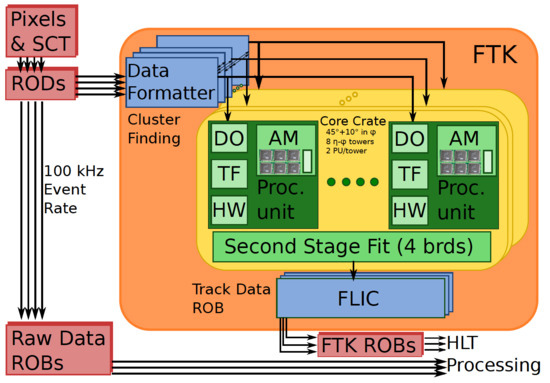
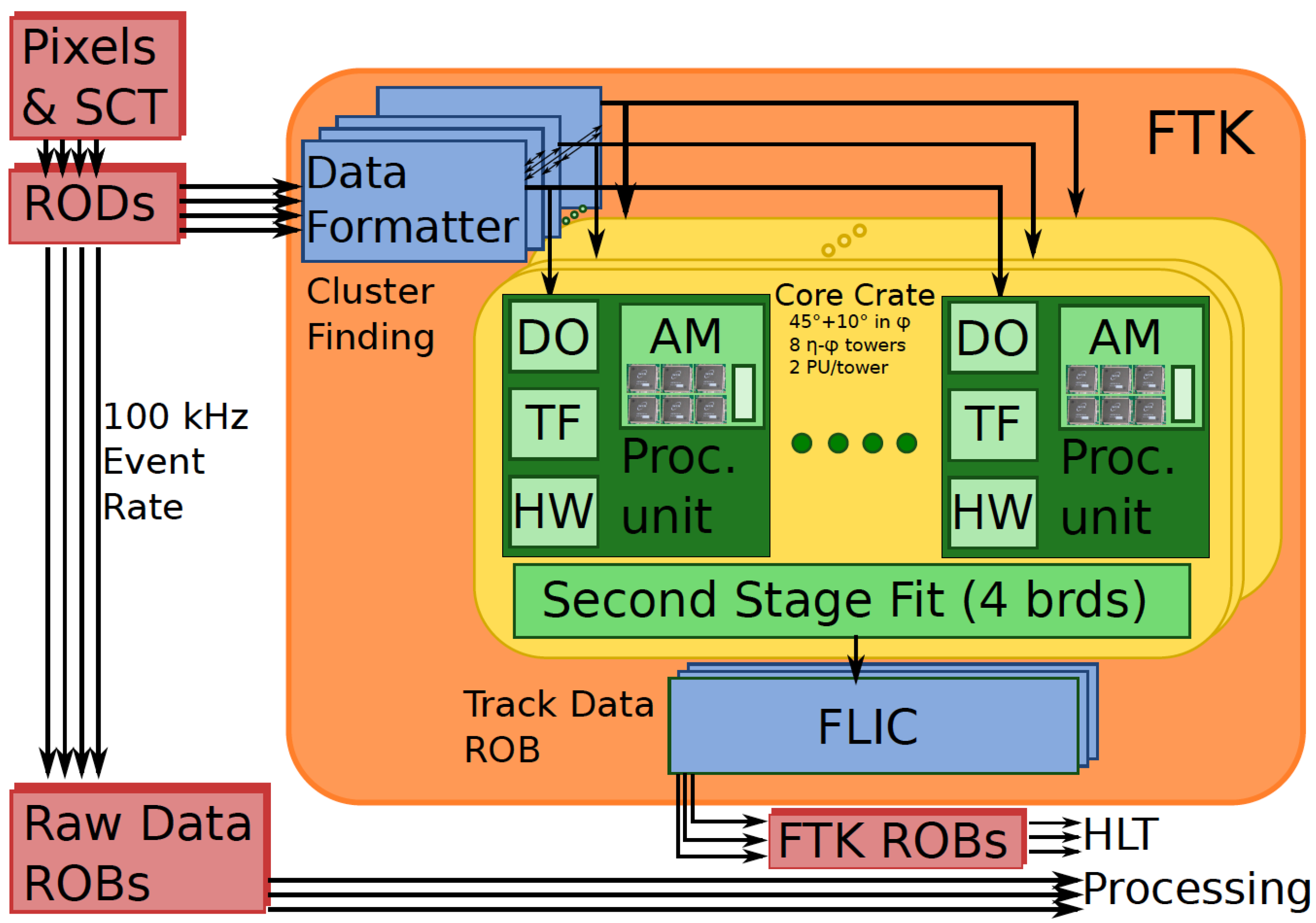
Figure 4 depicts a functional sketch of the FTK architecture. The large amount of data that the FTK receives from the silicon detectors, necessitates organizing the FTK as a set of independent processing engines, so that each engine corresponds to a different region of the silicon tracker. This organization is achieved with the segmentation of the tracker in 64 $\eta$-$\varphi$ regions, which are called “towers”.

The Pixel and Strip data are transmitted from the RODs to the Data Formatters (DF), through S-LINK fibers. Input Mezzanine (IM) boards, located on the DF, perform cluster finding (2-dimensional for the pixel layers; 1-dimensional for the strips). Clusters consist of neighboring pixels, linked diagonally or side-by-side. The DF groups the data based on the 64 $\eta$-$\varphi$ map of the silicon detector regions and transfers the cluster centroids (hits) to the corresponding Processing Unit (PU), which contains the AUXiliary board and the Associative Memory Board (AMB). Specifically, the hits are received by the AUX board, which stores them in the Data Organizer (DO) (a database built on the fly that relates the hits with the lower resolution Super Strips and allows a rapid retrieval of the hits in a Super Strip) and sends them to the AMB.

The AMB contains a large number of simulated Monte-Carlo patterns (> 10${}^9$), corresponding to all the relevant combinations of Super Strips. Each combination defines a possible track path through eight silicon layers—3 pixel layers (the B-layer and two outer pixel layers) and five SCT layers (four axial layers and one stereo layer). The simulated patterns are determined from a full simulation of the ATLAS detector with single tracks and are stored in Associative Memory chips [11] (AM chips) which hold 128k patterns each. Due to the fact that AM chips work in parallel, the pattern recognition in FTK finishes shortly after the last hit of the 8-layers is received from the silicon RODs. A pattern, which is matched in the data in all 8 or just 7 of the layers, defines a road containing a possible track. The AMB sends the road ID number to the DO, which sends this road ID number along with the full resolution hits to the Track Fitter (TF). The TF has access to a database which contains sets of pre-calculated constants, linearized by using a Principal Component Analysis (PCA) technique, for each detector sector. By using these constants, both the track helix parameters and the ${\chi }^2$, can be calculated as linear functions of the local hit coordinates. Nevertheless, in order to decide which track should be passed to the second stage, the first stage only calculates the ${\chi }^2$, not the helix parameters. Since in the first-stage there are 8 layers with a maximum of 11 measured coordinates (6 of them coming from the 3 pixel layers) and there are 5 helix parameters, the fit has 6 degrees of freedom and the ${\chi }^2$ is calculated as:

$${\chi }^2=\sum _{i=1}^6{\left(\sum _{j=1}^{11}{S}_{ij}{x}_j+h_i\right)}^2$$

(1)

where $S_{ij}$ and $h_i$ are the pre-calculated constants for this detector sector and $x_j$ are the local hit coordinates. To reduce the data sent to the second stage, the Hit Warrior (HW) removes the duplicate tracks which have already passed a ${\chi }^2$ requirement. Subsequently, the Second Stage Board (SSB) receives from the AUX board, the road ID number and the full resolution hits. The first-stage track is extrapolated to the additional 4 layers by the Extrapolator function of the SSB, where a minimum of 3 hits in the 4 layers is required, before a full 12-layer fit is performed. Both the ${\chi }^2$ and the helix parameters are determined this time. The track fitting is performed rapidly by the Track Fitter function of the SSB by using a simple linear calculation according to the following formula:

$$\widetilde{p_i}=\sum _{l=1}^N{c}_{il}{x}_l+q_i,\forall l=1\dots 5,$$

(2)

where, $\widetilde{p_i}$ are the 5 helix parameters, $c_{il}$ and $q_i$ are the pre-calculated constants for this detector sector and $x_l$ are the local hit coordinates.

After the second-stage fitting, a removal of duplicate tracks is carried out again for those tracks that passed a ${\chi }^2$ cut. There are two types of SSB, the preliminary (pSSB) and the final (fSSB), which have identical Extrapolator and Track Fitter functions, but only the fSSB performs removal of the duplicate tracks. The pSSB sends its tracks to the +$\varphi$-neighboring fSSB and the fSSB performs overlap removal for its own tracks and those received from the -$\varphi$-neighboring pSSB. The output of the fSSB contains the 12-layer hit tracks, the helix parameters, the ${\chi }^2$, and a word regarding the track quality which includes the layers with a hit. This output is received by the FTK-to-Level2 Interface Crate (FLIC) which organizes the tracks using the standard ATLAS protocols and sends them to the FTK ROSs.

2.3. FTK Infrastructure and Status

The FTK is currently being installed in the electronics room beside the ATLAS cavern. It is composed of 13 crates, consisting of 8 Versa Module Europa (VME) core crates and 5 Advanced Telecommunications Computing Architecture (ATCA) shelves.

The eight 9U VME core crates contain the AMBs, the AUX cards, and the SSBs. The four ATCA shelves with full-mesh backplanes carry the DF boards, while one ATCA shelf, with a dual-star backplane, contains the FLIC cards. The layout and the organization of an FTK core crate are shown in Figure 5. Each VME crate covers 45${}^{°}$ of the ATLAS detector in azimuth. There are 16 Processor Units (PU), 2 per FTK $\eta$-$\varphi$ tower, each consisting of an AMB with an AUX board connected behind it. Four PUs send eight-layer tracks to a common SSB. Each pair of SSBs transmits the twelve-layer tracks to the FLIC crate, which then sends them to the FTK ROSs.

Currently, FTK has integrated two “slices” into the ATLAS detector, and they regularly take data. Each slice corresponds to one $\eta$-$\varphi$ tower. The first slice, contains boards of each type, (four IMs on a DF, one AUX, one AMB, one SSB, one FLIC), fitting 12-layer tracks and the second slice contains the first half of the FTK chain (four IMs on a DF, one AUX, one AMB) giving 8-layer tracks as output. The FTK commissioning is on-going and data-taking is limited to the two slices mentioned above. In the 2-year LHC shutdown (2019–2020), FTK will continue the preparations for Run III of the LHC, when it should deliver tracks from the whole silicon detector region to the HLT. In parallel to the commissioning of the FTK hardware, the HLT infrastructure and algorithms are being prepared to make use of the FTK tracks. It is expected that the FTK will significantly enhance the physics potential of the ATLAS experiment. As an example, the use of FTK tracks in the HLT will drastically improve the efficiency of identifying taus from $H\to \tau \tau$ decays in the low-$p_T$ region below 30 GeV, where the current calorimeter-based HLT algorithms have a slow efficiency turn-on (for a collection of FTK results and performance expectations see [12]).

3. High-Level Data Quality Monitoring Framework

In the offline environment, Tier0 monitoring can perform a comparison between FTK tracks and offline tracks, or also compare HLT objects reconstructed with FTK tracks to those reconstructed with offline tracks. For online monitoring, FTK hardware specific information and physics event data in various processing stages, stored in the Spy Buffers of the FTK boards, are gathered, processed and presented by the monitoring facilities. However, there is a need to independently verify that the twelve-layer track outputs are functioning as expected on a track-by-track basis. The FTK High-Level Data Quality monitoring framework is used in order to confirm that the 12-layer tracks, produced by the FTK system, agrees with the expected tracks resulting from the FTK Simulation [13]. To achieve this, a comparison between these two output streams is performed and the histograms of this comparison are published to the Online Histogramming Service (OHS). This comparison is a simple way to detect non-expected output tracks from the FTK hardware. A general picture of this monitoring framework is presented in Figure 6.

A full event fragment is sampled by the Data Collection Manager (DCM) and acquired through the Event Monitoring (EMON) [14] service. The silicon detector data of this event serves as input for the FTK Simulation. The simulation dataflow processes the input event by following four basic algorithms. First, the clustering algorithm identifies the hit coordinates based on the firing pixels and strips of the detector and produces the list of clusters. Then, the data distribution algorithm simulates the Data Formatter hardware by geometrically distributing the clusters to the 64 FTK towers in order to be matched with the track patterns stored in AMBs. Next, the pattern matching algorithm reads these patterns and finds coincidences with clusters of the events. Finally, the track fitting reads the track candidates and searches for good tracks among the clusters. It extrapolates the good tracks into the additional four-layers and the tracks are collected and merged into a full event. After the FTK Simulation has finished, a comparison tool gets the simulated FTK tracks, extracts the real FTK hardware tracks, and performs a comparison between the parameters of these tracks. Based on the difference between the track parameters, four classes of histograms are created (completely matched tracks, slightly different tracks, tracks only in the FTK hardware stream, tracks only in the FTK simulation stream). After the comparison, the histograms are published to the OHS.

4. Conclusions

The ATLAS FTK is expected to provide high quality tracks to the HLT at the rate of 100 kHz. This will reduce the pile-up dependency of the system and improve the efficiency in the collection of interesting p-p collision events. It will also allow HLT to use more complex algorithms to look for particular signatures in the search for physics beyond the Standard Model. The integration with the ATLAS detector has already begun and the FTK is expected to fully operate during Run III of the LHC.

References

- ATLAS Collaboration. The ATLAS Experiment at the CERN Large Hadron Collider. J. Instrum. 2008, 3, S08003. [Google Scholar]
- ATLAS Collaboration. Observation of a new particle in the search for the Standard Model Higgs boson with the ATLAS detector at the LHC. Phys. Lett. B 2012, 716, 1–29. [Google Scholar] [CrossRef] [Green Version]
- ATLAS EXPERIMENT—Luminosity Public Results Run 2. Available online: https://twiki.cern.ch/twiki/bin/view/AtlasPublic/LuminosityPublicResultsRun2 (accessed on 30 November 2018).
- ATLAS Collaboration. ATLAS Level-1 Trigger: Technical Design Report; CERNLHCC-98-014, ATLAS-TDR-12. Available online: https://cds.cern.ch/record/381429 (accessed on 30 November 2018).
- ATLAS Collaboration. ATLAS High-Level Trigger, Data-Acquisition and Controls: Technical Design Report; CERN-LHCC-2003-022, ATLAS-TDR-16. Available online: https://cds.cern.ch/record/616089 (accessed on 30 November 2018).
- ATLAS Collaboration. ATLAS Inner Detector: Technical Design Report, 2; CERN-LHCC-97-017, ATLAS-TDR-5. Available online: https://cds.cern.ch/record/331064 (accessed on 30 November 2018).
- ATLAS IBL Collaboration. Production and Integration of the ATLAS Insertable BLayer. J. Instrum. 2008, 13, T05008. [Google Scholar]
- ATLAS Collaboration. Fast TracKer (FTK) Technical Design Report; CERN-LHCC-2013-007, ATLAS-TDR-025. Available online: https://cds.cern.ch/record/1552953 (accessed on 30 November 2018).
- Vazquez, W.P.; ATLAS Collaboration. The ATLAS Data Acquisition System in LHC Run 2. J. Phys. Conf. Ser. 2017, 898, 032017. [Google Scholar] [CrossRef] [Green Version]
- Annovi, A.; Castegnaro, A.; Giannetti, P.; Jiang, Z.; Luongo, C.; Pandini, C.; Roda, C.; Shochet, M.; Tompkins, L.; Volpi, G. Variable resolution Associative Memory optimization and simulation for the ATLAS FastTracker project. Proc. Sci. 2013, 13, 14. [Google Scholar] [CrossRef]
- Annovi, A.; Beretta, M.M.; Calderini, G.; Crescioli, F.; Frontini, L.; Liberali, V.; Shojaii, S.R.; Stabile, A. AM06: The Associative Memory chip for the Fast TracKer in the upgraded ATLAS detector. J. Instrum. 2017, 12, C04013. [Google Scholar] [CrossRef]
- ATLAS EXPERIMENT—FTK Public Results. Available online: https://twiki.cern.ch/twiki/bin/view/AtlasPublic/FTKPublicResults (accessed on 30 November 2018).
- Adelman, J.; Ancu, L.S.; Annovi, A.; Baines, J.; Britzger, D.; Ehrenfeld, W.; Giannetti, P.; Luongo, C.; Schmitt, S.; Stewart, G.; et al. ATLAS FTK Challenge: Simulation of a Billion-Fold Hardware Parallelism, ATL-DAQ-PROC-2014-030. Available online: https://cds.cern.ch/record/1951845 (accessed on 30 November 2018).
- Scholtes, I.; Kolos, S.; Zema, P.F. The ATLAS Event Monitoring Service—Peer-to-Peer Data Distribution in High-Energy Physics. IEEE Trans. Nucl. Sci. 2008, 55, 1610–1620. [Google Scholar] [CrossRef]
Figure 1.
(a) Cumulative luminosity versus day for 2011-2018 delivered to ATLAS during stable beams for high energy p-p collisions [3]. (b) Mean number of Interactions per Crossing, showing the 13 TeV data from 2015–2018 [3].
Figure 2.
The ATLAS DAQ System in LHC Run 2 [9].
Figure 3.
The FTK receives raw hits from the Inner Detector and provides to HLT reconstructed 12-layer tracks.
Figure 4.
Functional sketch of FTK. AM is the Associative Memory, DO is the Data Organizer, FLIC is the FTK-to-Level-2 Interface Crate, HW is the Hit Warrior, ROB is the ATLAS Read Out input Buffer, ROD is a silicon detector Read Out Driver, and TF is the Track Fitter. Second Stage Fit is referred to as the Second Stage Board elsewhere in the document.
Figure 5.
Layout of an FTK core crate and the interboard and intercrate data flow.
Figure 6.
Layout of the High-Level Data Quality Monitoring Framework.
© 2019 by the author. Licensee MDPI, Basel, Switzerland. This article is an open access article distributed under the terms and conditions of the Creative Commons Attribution (CC BY) license (http://creativecommons.org/licenses/by/4.0/).
Share and Cite
MDPI and ACS Style
Marantis, A., on Behalf of the ATLAS Collaboration. The ATLAS Fast TracKer—Architecture, Status and High-Level Data Quality Monitoring Framework. Universe 2019, 5, 32. https://doi.org/10.3390/universe5010032
AMA Style
Marantis A on Behalf of the ATLAS Collaboration. The ATLAS Fast TracKer—Architecture, Status and High-Level Data Quality Monitoring Framework. Universe. 2019; 5(1):32. https://doi.org/10.3390/universe5010032
Chicago/Turabian StyleMarantis, Alexandros, on Behalf of the ATLAS Collaboration. 2019. "The ATLAS Fast TracKer—Architecture, Status and High-Level Data Quality Monitoring Framework" Universe 5, no. 1: 32. https://doi.org/10.3390/universe5010032
Note that from the first issue of 2016, this journal uses article numbers instead of page numbers. See further details here.