Quantum Cramer–Rao Bound for a Massless Scalar Field in de Sitter Space

Department of Physics, Graduate School of Science, Nagoya University, Chikusa, Nagoya 464-8602, Japan
*
Author to whom correspondence should be addressed.
Universe 2017, 3(4), 71; https://doi.org/10.3390/universe3040071
Submission received: 31 July 2017
/
Revised: 6 October 2017
/
Accepted: 10 October 2017
/
Published: 13 October 2017
Abstract
:How precisely can we estimate cosmological parameters by performing a quantum measurement on a cosmological quantum state? In quantum estimation theory, the variance of an unbiased parameter estimator is bounded from below by the inverse of measurement-dependent Fisher information and ultimately by quantum Fisher information, which is the maximization of the former over all positive operator-valued measurements. Such bound is known as the quantum Cramer –Rao bound. We consider the evolution of a massless scalar field with Bunch–Davies vacuum in a spatially flat FLRW spacetime, which results in a two-mode squeezed vacuum out-state for each field wave number mode. We obtain the expressions of the quantum Fisher information as well as the Fisher informations associated to occupation number measurement and power spectrum measurement, and show the specific results of their evolution for pure de Sitter expansion and de Sitter expansion followed by a radiation-dominated phase as examples. We will discuss these results from the point of view of the quantum-to-classical transition of cosmological perturbations and show quantitatively how this transition and the residual quantum correlations affect the bound on the precision.
1. Introduction
Particle creation associated with cosmological expansion is a long-studied topic in the literature [1]. Special attention has been paid to the case of the FLRW metrics used in cosmology [2]—in particular to the maximally symmetric case of the de Sitter spacetime for its role in modeling the early inflationary phase of the universe and the dark-energy-dominated expansion at late times. We would like to consider the evolution of such quantum cosmological states from the point of view of cosmological parameter estimation. Previous work on parameter estimation in cosmological models has been carried out for example in [3] for a Milne universe described by an expansion law with flat limit in the asymptotic past and asymptotic future regions [4]. Nevertheless, while entropic properties of scalar and spinor fields in FLRW metric have been considered in works such as [5,6], an analysis of information about the parameters of the cosmological information is still missing. Furthermore, while the effect of the quantum-to-classical transition of cosmological perturbations has been widely discussed [7,8,9,10], its effect on the information we can retrieve from them about cosmological parameters has not yet been considered.
The main focus of the present work is to study the higher bound put on how precisely we are allowed to estimate a generic cosmological parameter by performing a chosen quantum measurement on the out-state of a massless scalar Bunch–Davies vacuum in FLRW space-time. In the specific de Sitter case, we might identify the scalar field with perturbations of the inflaton field. In parameter estimation theory, the lower bound for the variance of an unbiased parameter estimator for a given measurement is provided by the Cramer–Rao bound as the inverse of the Fisher information. In the context of quantum estimation, quantum Fisher information is defined as the maximization of the Fisher information over all choices of quantum measurements. We obtain and discuss the expressions of the quantum Fisher information and the Fisher informations for the occupation number measurement and the power spectrum measurement, with special emphasis on the behavior in the pure de Sitter expansion and de Sitter phase followed by a radiation-dominated phase for the estimation of the Hubble parameter. Furthermore, we will provide some considerations on how the results can be considered from the point of view of how the quantum-to-classical transition of the inflaton field perturbations affects the estimation precision.
The paper is structured as follows. In Section 2, we quickly review the solution of the equation of motion for a massless scalar field in de Sitter space with Bunch–Davies vacuum and introduce the Wigner function description of the resulting two-mode squeezed vacua. In Section 3, we remind the reader of the definition of Fisher information in classical and quantum estimation theory [11], and we provide its evaluation for the measurement of the occupation number and the field mode amplitude of the scalar field, together with its maximization over all quantum measurements. In Section 4 we show the specific results for the Hubble parameter estimation in the pure de Sitter case and for the case of de Sitter expansion followed by a radiation-dominated phase, which show significant differences. Finally, in Section 5, we address the relation of the results for the Fisher information with the quantum-to-classical transition of cosmological perturbations, providing final observations and conclusions in Section 6.
2. Massless Scalar Field in an Expanding Universe
Consider a massless minimally coupled scalar field in a spatially flat FLRW universe of metric
with the scale factor a and the conformal time . The Lagrangian for this field, rescaled as , is given by
where . This Lagrangian leads to equations of motion of the form
We introduce the Fourier mode of the field and its conjugate momentum as
where . Following the usual quantization procedure, we express the field mode and conjugate momentum in terms of the time-dependent creation and annihilation operators and
so that we can express the Hamiltonian as
where in order to treat and modes as independent variables, integral over is performed in half the Fourier space, . The Heisenberg equations of motion for the operators and for the modes are
where . In the Heisenberg formalism, the relation between operators at a given conformal time and at a later time is given by the Bogoliubov transformation
where and are the Bogoliubov coefficients satisfying with initial conditions and . The time evolution of these coefficients is obtained straightforwardly from (8)
We define the vacuum state as the eigenstate of the annihilation operator at time
Introducing the Schrödinger picture of the state at , the transformation (9) gives the vacuum condition
the solution of which provides the the out-state
In the following, we will consider only the component for a fixed value of k, as different modes do not interact with each other in the linear order. For each value of k, components of (13) are two-mode () squeezed vacuum states, with squeezing parameters related to the Bogoliubov coefficients by
being a free phase. For simplicity of notation, in the following we will omit the index k in the parameters.
The squeezing magnitude r and phase follow the evolution equations
In the basis that diagonalizes , the vacuum condition (12) provides the Gaussian wave function
where . In order to deal with real coordinates, in the following we will introduce Hermitian field mode variables and as
and analogously for the variables in . In the basis that diagonalizes , the wave function reads
It is convenient to consider the Wigner function associated to the wave function of the pure state for which explicit calculation gives the Gaussian distribution
where we have defined and is the covariance matrix, which specifies completely the state and can be expressed in the block form as
and being Pauli matrices and the identity matrix.
3. Fisher Information of the Scalar Field
In order to discuss the bound on the estimation precision, we consider the Fisher information. In the classical case, let be the probability distribution to obtain a certain measurement result x, parametrized by a single scalar . The Cramer–Rao bound provides a lower bound for the variance of the estimator of the parameter through the single measurement of a variable x
where and is the Fisher information defined by
For simplicity, we consider a single scalar parameter , but the extension to the multiparameter case is straightforward.
In the context of quantum estimation theory [11], the Fisher information can be expressed in terms of a positive operator-valued measurement . For a state parametrized by the quantity , the result of the measurement has probability distribution and the Fisher information is
where one makes use of the symmetric logarithmic derivative (SLD) , a self-adjoint operator implicitly defined by
The Fisher information can be shown to be maximized over all positive operator-valued measurements by the quantum Fisher information
which provides the ultimate quantum Cramer–Rao bound
with the equality being satisfied when the measurement projects over the eigenstates of the SLD operator. For a pure state , and
Hence, the SLD operator takes the simple form
Therefore, for the pure state, the quantum Fisher information can be expressed as
For our purposes, we can restrict ourselves to consider a pure Gaussian state (i.e., a quantum state with Gaussian Wigner function) whose wave function and Wigner function are given by (19) and (20), respectively (for a reference on quantum estimation theory using single-mode Gaussian states, see e.g., [12]). By taking derivative of the Wigner function W with respect to a parameter ,
it is possible to show that
and the quantum Fisher information can be expressed in terms of the covariance matrix as
For the covariance matrix (21), we obtain
Let us now consider specific measurements of the scalar field. A first natural choice could be to evaluate the Fisher information for the projective measurement of the occupation number,
The state after the measurement is
with measurement outcome probability
We found that the Fisher information associated to (37) is simply
This shows that the number measurement is allowed to access the part of quantum Fisher information associated to the parameter-dependency of the squeezing magnitude, but not that associated to the parameter-dependency of the squeezing phase. In other words, the number measurement allows the highest precision for the estimation of a cosmological parameter as long as the squeezing phase of the state does not depend on that parameter, which generally does.
To have a better insight into the effect of decoherence on the allowed estimation precision, which we will discuss in Section 5, let us consider also the measurement of the power spectrum of the field (i.e., the modulus squared of the amplitude of its modes). For this purpose, we introduce new variables as
The original field mode is expressed as
From the Wigner function (20), by integrating over , the marginal probability distribution for variables is obtained
As the operators associated to commute, it is possible to measure these variables simultaneously by homodyne detection for the quadratures (notice that choice of variables corresponds to the measurement of conjugate momentum amplitude). The Fisher information for the probability distribution (41) is
where the contributions from parameter-dependency of the squeeze magnitude and squeeze phase are now mixed.
Notice that the Fisher information for the power spectrum measurement is related to the strength of correlations between the and modes, which are given by the expectation value for the field mode amplitude
since . By writing explicitly the wave function in the representation, it is possible to show that these correlations can be expressed in terms of the Bogoliubov coefficients simply as
and therefore from (42) one has
The correlations (43) may be compared to the ones associated to the projection of the state on the number basis
In the limit of large squeezing, these correlations are related as
The correlations (43) and (46) are related to the Shannon entropy of the respective measurement distributions as follows. The probability density function of the power spectrum of the field is
which has the following Shannon entropy
This provides us with the simple relation between the Fisher information and the Shannon entropy for field mode amplitude
The entropy for the number state projection is
which coincides with the entropy of entanglement between and modes. In the large squeezing limit, we then have
As we will explain in Section 5, the value corresponds to the maximal attainable value of the entropy via coarse graining of the state with complete randomization. Notice that the result (50) is exact and directly relates the Fisher information for the power spectrum measurement to the field entropy.
4. Fisher Information in de Sitter Universe
As an example of the results of the previous section, let us consider a pure de Sitter space-time with conformal factor . For the Bunch–Davies vacuum, the Bogoliubov coefficients are
The squeezing parameters are
Fisher informations are given by
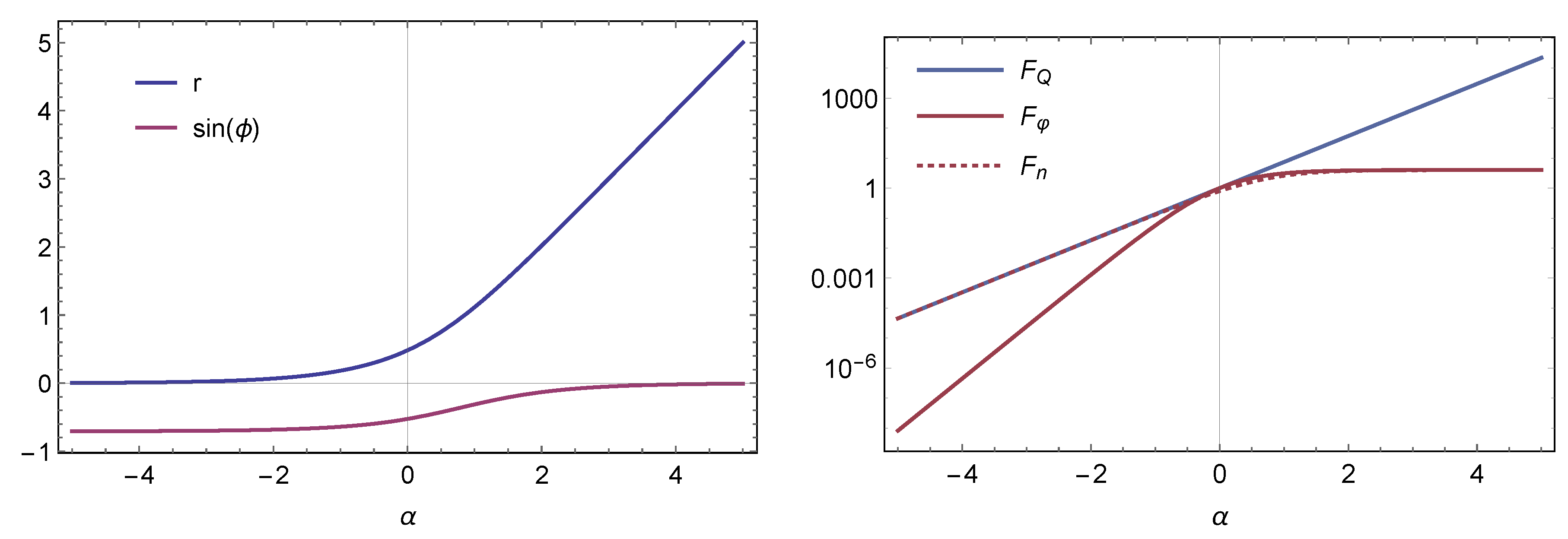
where is the e-foldings of cosmic expansion and represents the parameter dependence of the e-foldings. Figure 1 (left panel) shows the evolution of the squeezing parameter and squeezing phase. When the physical wavelength is smaller than the Hubble horizon (i.e., for modes inside the Hubble horizon), the squeezing parameter and phase are constant. After the horizon exit at , we have and r grows while approaches zero.
In the super-horizon scale , these Fisher informations behave as
On the other side, in the small scale , we have
Thus, we obtain the relation
As the state is squeezed more and more in the super horizon scale, most of the quantum Fisher information becomes inaccessible to either of the measurements. As we discussed before, the difference between and is due to the parameter dependency of the squeezing phase . As one may notice by looking at the covariance matrix (21), obtaining such information requires a measurement that properly accesses the correlations between the and modes, represented by the off-diagonal blocks of the matrix. Notice that for any given k-mode, the squeezing phase is related to the quantum phases of the two modes of the squeezed vacuum in the number representation by , where is the operator appearing at exponent in the Pegg–Barnett phase operator, acting on the modes [13].
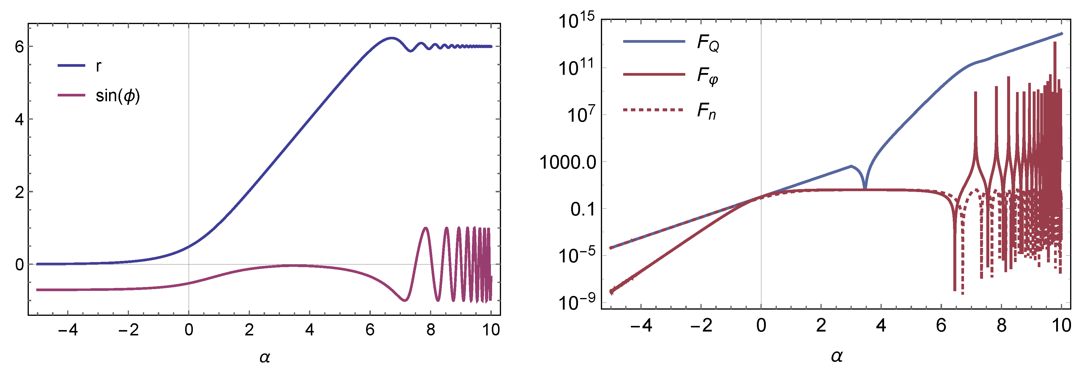
Now let us consider a cosmological model with transition from de Sitter expansion to decelerated expansion (radiation-dominated phase). The scale factor in this case is
Figure 2 shows the evolution of squeezing parameters and Fisher informations for the mode. The transition from de Sitter expansion to decelerated expansion is at , which corresponds to .
During the de Sitter phase, the physical wavelength of this mode exceeds the Hubble horizon length. After , the wavelength again becomes smaller than the Hubble horizon length, and after this time, the squeezing magnitude and phase start to oscillate, as already observed in [14]. After the reentry of the mode in the Hubble horizon, Fisher informations and also oscillate. In particular, the Fisher information reaches the same values as for some values of . This means that there is the possibility that the estimation through measurement of the power spectrum can attain the quantum Cramer–Rao bound. The reason for this is that in the radiation-dominated era, a contour of the Wigner function becomes an elongated ellipse with fixed hlaxes (since r approaches a constant value) and rotates in the phase space in such a way that at some point it becomes completely accessible to the measurement of quadratures . The equality holds for
Thus, if we consider the homodyne measurement of the field quadrature, we have a chance to attain the quantum Cramer–Rao bound periodically in time. On the other hand, the amplitude of keeps the same maximal value when the mode is outside of the Hubble horizon, and this value is far smaller than the value of in the radiation-dominated era.
5. Quantum-to-Classical Transition of Cosmological Perturbations
In the previous sections, we have considered the amount of quantum Fisher information of a cosmological parameter that is accessible by performing two different projective measurements on the pure cosmological state. In this case, the fact that not all of the quantum Fisher information for the parameter can be accessed is ascribed to the fact that the choice of measurement is non-optimal, in the sense that it does not satisfy the equality in the quantum Cramer–Rao bound (27). Now, we would like to adopt a different point of view and see the projection over the chosen set of states as representing the interaction of the cosmological state with an external environment rather than with an observer. From this point of view, the fact that quantum Fisher information becomes partially inaccessible is ascribed to the entanglement of the initially pure state with the degrees of freedom of the environment, which are inaccessible to the observer. As a consequence, to such an observer the state will appear not pure but mixed.
The motivation behind this slight change of perspective is that the field mode amplitude states that we considered can be taken approximatively as the pointer basis of the evolution of cosmological perturbations; i.e., the basis “naturally chosen” by the interaction with the environment leading from quantum perturbations to classical ones [14]. This environment-induced interpretation of the information loss requires the interaction to be strong enough as to be analogous to an instantaneous projective measurement. Such interaction of the cosmological system with the environment is a realistic consideration, in particular when one takes into account the frailty of squeezing [8]. The interaction with the environment can be generically modeled by attaching a dumping factor to the initial pure state
being a parameter that encodes the details of the interaction. The decoherence from the initial pure state to the final mixed state can be quantified by the von Neumann entropy of the total state (61). In the limit , [14] found
when expressed in the present notation. By substituting (49), taking the limit for large squeezing, we have the following relation:
where represents the maximum value of the entropy for this bipartite system. In terms of the Wigner function, this value is obtained by smearing the Wigner ellipse to become a circle. As discussed in [14], such a bound shows that the reduction over the field amplitude pointer states does not lead to complete quantum decoherence but retains some amount of “quantumness”.
From the point of view of decoherence, as a result of the quantum-to-classical transition of cosmological perturbations, the quantum Fisher information for the local system is reduced from the initial to a lower value after the transition, power spectrum becoming the optimal measurement in terms of parameter estimation. Corresponding to this decrease in quantum Fisher information, there is an increase in the von Neumann entropy from its minimal value of zero for the initial pure state to its maximal value of . Notwithstanding this cosmological decoherence, the interaction with the environment does not lead to total loss of quantum correlations, whose contribution to the final quantum Fisher information can be determined as . In the radiation-dominated case, such contributions periodically allow access to all of the Fisher information of the cosmological parameter that presented before the quantum-to-classical transition through a measurement of power spectrum, while this information is lost in the limit of pure de Sitter space. Notice that in the large squeezing limit, the entropy consistently shows log-periodic fluctuations due to the factor in (47), and such fluctuations disappear in the large squeezing limit of the de Sitter case, where and .
One may observe then that the fact that the mechanism of cosmological decoherence is not perfectly efficient turns out to be extremely important from the point of view of observation, not only for generating observable features such as the acoustic peaks in the anisotropy spectrum of the CMB (as observed in [10]), but also for being determinant in how well we can estimate cosmological parameters from our observations by accessing quantum correlations by a proper choice of the measurement.
6. Conclusions
In conclusion, constraining ourselves to the case of the massless Bunch–Davies scalar vacuum in a FLRW metric parametrized by some scalar cosmological parameter, we found the explicit expressions for the quantum Fisher information and the Fisher informations associated to the measurement of the power spectrum and occupation number, both in terms of the Bugoliubov coefficients of the cosmological unitary transformation and in terms of the squeezing magnitude and phase of the two-mode squeezed out-vacuum state. While quantum Fisher information cannot be accessed completely by the two chosen measurements in the pure de Sitter case, it can be accessed periodically by the power spectrum measurement when we introduce a radiation-dominated phase, such periodicity being related to the rotation of the Wigner function in the quantum phase space. In the context of the quantum-to-classical transition of cosmological perturbations, we have shown quantitatively how the transition affects the value of the quantum Fisher information before and after the cosmological decoherence, as well as how the residual quantumness of the correlations of the final state contribute to it.
Notice that the periodicity of the saturation of the quantum Cramer–Rao bound is both in conformal time and field wavenumber. That is, for a fixed conformal time we can find a specific value of the field mode that satisfies (60), preserves the total quantum Fisher information, and whose observation allows the highest estimation precision. These results can be straightforwardly extended to the multi-parameter case and model-specific conformal factors. From a more theoretical point of view, since bosonic and fermionic cosmological particle creation show qualitatively different entanglement behaviors, it could be interesting to study the same problem for fermionic fields.
Acknowledgments
Y.N. was supported in part by JSPS KAKENHI Grant Number 16H01094. M.R. gratefully acknowledges support from the Ministry of Education, Culture, Sports, Science and Technology (MEXT) of Japan.
Author Contributions
Both authors contributed equally to this work. Both authors have read and approved the final manuscript.
Conflicts of Interest
The authors declare no conflict of interest.
References
- Birrell, N.D.; Davies, P.C.W. Quantum Fields in Curved Space; Cambridge University Press: Cambridge, UK, 1982. [Google Scholar]
- Liddle, A.R.; Lyth, D.H. Cosmological Inflation and Large-Scale Structure; Cambridge University Press: Cambridge, UK, 2000. [Google Scholar]
- Wang, J.; Tian, Z.; Jing, J.; Fan, H. Parameter estimation for an expanding universe. Nucl. Phys. B 2015, 892, 390–399. [Google Scholar] [CrossRef]
- Duncan, A. Explicit dimensional renormalization of quantum field theory in curved space-time. Phys. Rev. D 1978, 17, 964. [Google Scholar] [CrossRef]
- Ball, J.L.; Fuentes-Schuller, I.; Schuller, F.P. Entanglement in an expanding spacetime. Phys. Lett. A 2006, 359, 550–554. [Google Scholar] [CrossRef]
- Fuentes, I.; Mann, R.B.; Martin-Martinez, Y.; Moradi, S. Entanglement of Dirac fields in an expanding spacetime. Phys. Rev. D 2010, 82, 045030. [Google Scholar] [CrossRef]
- Zeh, H.D. Decoherence and the Appearance of a Classical World in Quantum Theory; Springer: Berlin, Germany, 1996. [Google Scholar]
- Polarski, D.; Starobinsky, A. Semiclassicality and decoherence of cosmological perturbations. Class. Quantum Gravity 1996, 13, 377–391. [Google Scholar] [CrossRef]
- Campo, D.; Parentani, R. Inflationary spectra and partially decohered distributions. Phys. Rev. D 2005, 72, 045015. [Google Scholar] [CrossRef]
- Kiefer, C.; Polarski, D. Why do cosmological perturbations look classical to us? Adv. Sci. Lett. 2009, 2, 164. [Google Scholar] [CrossRef]
- Paris, M.G.A. Quantum estimation for quantum technology. Int. J. Quantum Inf. 2009, 7 (Suppl. 1), 125–137. [Google Scholar] [CrossRef]
- Pinel, O.; Jian, P.; Treps, N.; Fabre, C.; Braun, D. Quantum parameter estimation using general single-mode Gaussian states. Phys. Rev. A 2013, 88, 040102. [Google Scholar] [CrossRef]
- Gantsog, Ts.; Tanaś, R. Phase properties of the two-mode squeezed vacuum states. Phys. Lett. A 1991, 152, 251–256. [Google Scholar] [CrossRef]
- Kiefer, C.; Lohmar, I.; Polarski, D.; Starobinsky, A. Pointer states for primordial fluctuations in inflationary cosmology. Class. Quantum Gravity 2007, 24, 1699–1718. [Google Scholar] [CrossRef]
Figure 1.
(Left) Evolution of squeezing parameter and squeezing phase for ; (Right) Evolution of Fisher informations divided by for .
Figure 1.
(Left) Evolution of squeezing parameter and squeezing phase for ; (Right) Evolution of Fisher informations divided by for .

Figure 2.
(Left) Evolution of squeezing parameters for ; (Right) Evolution of Fisher informations divided by for .
Figure 2.
(Left) Evolution of squeezing parameters for ; (Right) Evolution of Fisher informations divided by for .

© 2017 by the authors. Licensee MDPI, Basel, Switzerland. This article is an open access article distributed under the terms and conditions of the Creative Commons Attribution (CC BY) license (http://creativecommons.org/licenses/by/4.0/).
Share and Cite
MDPI and ACS Style
Rotondo, M.; Nambu, Y. Quantum Cramer–Rao Bound for a Massless Scalar Field in de Sitter Space. Universe 2017, 3, 71. https://doi.org/10.3390/universe3040071
AMA Style
Rotondo M, Nambu Y. Quantum Cramer–Rao Bound for a Massless Scalar Field in de Sitter Space. Universe. 2017; 3(4):71. https://doi.org/10.3390/universe3040071
Chicago/Turabian StyleRotondo, Marcello, and Yasusada Nambu. 2017. "Quantum Cramer–Rao Bound for a Massless Scalar Field in de Sitter Space" Universe 3, no. 4: 71. https://doi.org/10.3390/universe3040071
Note that from the first issue of 2016, this journal uses article numbers instead of page numbers. See further details here.