Baryon Number Transfer Could Delay Quark–Hadron Transition in Cosmology

Abstract

In the early Universe, strongly interacting matter was a quark–gluon plasma. Both lattice computations and heavy ion collision experiments, however, tell us that, in the absence of chemical potentials, no plasma survives at $T<\sim 150$ MeV. The cosmological Quark–Hadron transition, however, seems to have been a crossover; cosmological consequences envisaged when it was believed to be a phase transition no longer hold. In this paper, we discuss whether even a crossover transition can leave an imprint that cosmological observations can seek or, vice versa, if there are questions cosmology should address to QCD specialists. In particular, we argue that it is still unclear how baryons (not hadrons) could form at the cosmological transition. A critical role should be played by diquark states, whose abundance in the early plasma needs to be accurately evaluated. We estimate that, if the number of quarks belonging to a diquark state, at the beginning of the cosmological transition, is $<\sim 1:{10}^6$, its dynamics could be modified by the process of B-transfer from plasma to hadrons. In turn, by assuming B-transfer to cause just mild perturbations and, in particular, no entropy input, we study the deviations from the tracking regime, in the frame of SCDEW models. We find that, in some cases, residual deviations could propagate down to primeval nuclesynthesis.

1. Introduction

The number of strongly interacting (s.i.) particles in the present Universe appears negligible. They are mostly protons and neutrons, sometimes embedded in nuclides, whose mutual distance, on average, exceeds 1m. For the sake of comparison, in a cubic cm, there are more than 400 photons.

The drastic decline of s.i. particle number density occurred at $T\sim 150$ MeV, when the primeval Quark–Gluon (QG) plasma ceased to make part of the thermal soup. In the 1980s, when early lattice results on QG plasma (see, e.g., [1,2]) seemed to indicate that the transition from plasma to hadron gas was a real first order phase transition, and a large number of papers was devoted to study this transition in the cosmological context. A comprehensive list can be found in the review paper [3].

Attention then declined when lattice computations, including three quark flavors and tentatively considering also dynamical fermions, begun to make clear that, in the cosmological context, we had a crossover transition. As a consequence, most of the envisaged observational consequences on DM nature [4] and, namely, on Big-Bang-Nucleosynthesis (BBN; see [5,6]), loosed their motivation.

We do not intend to revitalize these arguments here. The central point of this paper will concern the B transfer from primeval plasma to hadronic gas, focusing on problems this could cause and formulating a question that lattice computations, hopefully, can answer. In spite of this, it is useful to recall why BBN was believed to be potentially affected by the QH transition: the point is that BBN occurs when the scale factor has increased less than a factor ${10}^3$ from the time of the transition. If the transition had been first order, according to Witten evaluations [4], the baryon number B could have tended to remain in the plasma bubbles which finally shrank into quark nuggets, surviving until now and yielding DM. It soon became clear, however, that even such remnants could not escape a final transition into hadron matter; the process, however, yielded a strong B concentration in the nugget sites. According to [5], the resulting B inhomogeneities could yield proton peaks, lasting until BBN, while residual neutrons reached homogenity by then.

In spite of the present common wisdom on the nature of QH transition, the option of an inhomogeneous BBN has also often been considered in recent literature, meaning that, at the opening of the so-called deuterium bottleneck, proton distribution was still inhomogeneous, so that neutrons had to flow back in proton concentration sites before being able to yield ${}^2$H nuclides (see, e.g., [7]).

Altogether, let us outline that there exist at least four contexts in which the QH transition is debated. Besides the cited cosmological and computational lattice contexts, there exists another astrophysical possibility, the transition of neutron stars into quark stars (e.g., [8,9]), although no conclusive word has ever been said on the energy gain allowed when B is carried also by strange quarks, besides $up$ and $down$ forming ordinary nucleons. Finally, a highly significant new field of research has been opened up by the study of heavy ion collisions, namely by LHC and RHIC experiments (for a discussion see, e.g., [10])

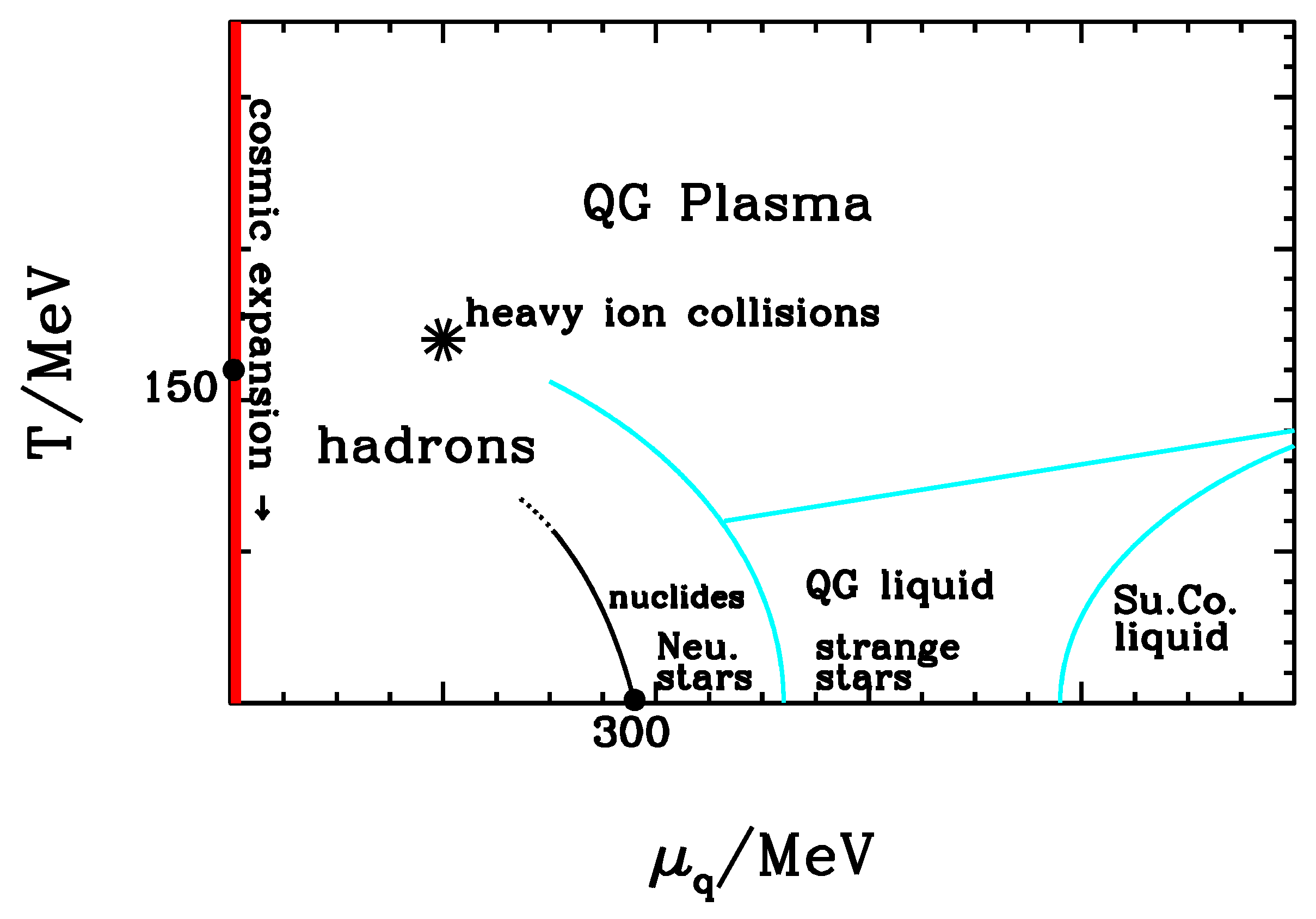
Unfortunately, however, the only tool to relate laboratory and cosmic data is numerical QCD, as each cosmic context and laboratory outputs are scarsely communicating; the very scheme in Figure 1, sometimes shown in general talks to show the connections among different contexts, is still highly hypothetical. In turn, in spite of the huge progress realized in lattice computation, they are still unable to fully meet some simple datasets.

In spite of that, we can make two points that, in our opinion, did not receive enough attention in previous literature, while being potentially significant. In the next section, we shall deal with the former of these points, concerning the transfer of B from primeval plasma to confined baryons; this will enable us to formulate specific questions, concerning diquark states, that lattice computations and heavy ion collision physics might try to answer. In Section 3, we shall somehow invert the perspective, and discuss the behavior of coupled DM–DE, in SCDEW models (see, e.g., [12,13]), across the cosmological QH transition. The basic merit and problem of these cosmologies is that they avoid the conceptual problems of ΛCDM while keeping its successes, so that they can be hardly discriminated from them. Accordingly, the search of observables that SCDEW could affect bears a significance, even though current observational errors still cover the signals. Section 4 will be devoted to draw specific conclusions on both topics.

2. Baryon Number Transfer from Plasma to Baryons, and Likelihood of Diquark States

The nuggets of quarks envisaged by Witten, if real, would ease the transfer of the extremely diluted baryon number from QG plasma into three-quark baryons. If the QH transition is a crossover, the transfer could be more intricate.

We can, however, imagine an ideal process, allowing a smooth B-transfer. If the whole plasma could directly turn into hadron gas, ∼$5\%$–$10\%$ of the newly formed gas would be made by baryons and antibaryons, separately forming by sticking together three suitably colored quarks and antiquarks. Successively, most baryons and antibaryons mutually annihilate, thus leaving the fair amount of residual baryons. Let us address this sequence of events as “option A”.

In turn, if only quark–antiquark bosonic doublets could form and no (anti)baryonic triplets were synthetized, the transition would be simply inhibited, as the Universe cannot remain with a residual of unconfined quarks whose mutual distance is ∼1000 times the confinement distance. Let us address this ideal scenario as “option 0”.

What actually occurred is intermediate between these extreme options and, unfortunately, closer to the “option 0”. As is known, most of the entropy of the QG plasma (initially ∼$69\%$ of the total) has to turn into photon–lepton entropy, as the hadron gas will end up with <$3\%$ of the total entropy (more details on this latter estimate are provided below). The point is then that the timing of photon–lepton entropy production, far from being arbitrary, is established by Friedmann equations, requiring the main reactions occurring at the transition to be direct quark–antiquark annihilations into photon–lepton pairs.

Freshly formed photons and leptons then infiltrate in the plasma. They have no proper volume, however, and the presence of residual quarks and antiquarks is no problem unless the overall (confined and unconfined) quark number density shifts below ∼$T_c^3$. This limit, however, cannot be overcome unless B is fully transferred to baryonic triplets. This must occur while the share of reactions sticking together free (anti)quarks into (anti)baryonic triplets has reduced by 1–2 orders of magnitude, so that we approach the “option 0”.

The smooth crossover transition envisaged by lattice calculations and tested in heavy ion collisions could then not coincide with what took place in the cosmological context.

Of course, it is simply impossible that color charges become isolated. If cosmic evolution approaches such a situation, what would occur is that the color dielectric constant would reduce, so that the enlarged color electric field produces lots of soft gluons. Because of the non-abelian nature of the gluon field, they will instantly form strings connecting and neutralising the color charges. Their length being large enough, they then decay in new quark–antiquark pairs leading to a chain of hadrons. The cosmological meaning of this series of event is that the Universe has gone out of equilibrium and the final output would be a substantial entropy input.

B transfer could be, however, facilitated by the presence of di–quark states. Truly confined quark couples arise only from the union of quark and antiquark; however, besides these straight couples, we ought to believe that, at least initially, there forms some homo couples, made of two quarks or two antiquarks and that a fair amount of them survives collisions and mutual annihilation.

Similar anomalous couples, named diquarks, have indeed been widely studied in recent literature. They were originally devised by [14] but really revitalized by [15], when suggesting that they would provide an explanation for an exotic baryon antidecuplet, the ${\Theta }^{+}$, whose evidence had been reported by the LEPS collaboration [16]; objections were soon raised by [17]; meanwhile, the matter has almost been settled, and, for a general review, see, e.g., [18]). Diquark evidence in lattice QCD was then soon outlined by [19]. For a general discussion on diquark properties, see [20,21,22].

Let us add that more experimental evidence came in later years. For a recent discussion, see [23] and references therein. In turn, baryon form factor analysis also seems to indicate that protons are to be seen as quark–diquark bound states (see, e.g., [24]). In addition, diquarks are the central ingredient of the dense QG matter yielding a color superconductor (see Figure 1).

If quark–diquark collisions are the basic process responsible for B transfer, we can perform a rough estimate of which fraction f of quarks should keep a homo partner, when approaching $T_c$. In fact, the mean free path of free quarks, for collisions with diquarks, reads

$${\lambda }_2\simeq \frac{1}{\sigma n_{b}f}$$

(1)

with $n_b\simeq {10}^{-9}n$ (here, $n=(\zeta \left(3\right)/{\pi }^2)15.75T_c^3\sim T_c^3$ is the quark number density at $T_c$) and $\sigma \sim T_c^{-2}$. Accordingly, if we require ${\lambda }_2\ll {10}^3$cm (∼$1/10$ – $1/100$ of the horizon at $T_c$), we conclude that, if

$$f<\sim {10}^{-6},$$

(2)

baryon forming could significantly interfere with the dynamics of the cosmological transition. Of course, not all collisions will be effective, for energetic and/or color matching reasons. This, however, does not change the order of magnitude of the estimate. Furthermore, there will be the same rate of collisions with antiquark pairs, but they hardly matter, as they are expected to yield just a straight couple and leave a residual uncoupled B-carrying quark.

Anyhow, unless all B is transferred so that the “risk” of residual free quarks is over, the overall quark number density cannot decrease much below $T_c^3$.

Elementary processes being too slow to allow the Universe to remain in a full equilibrium state are a recurrent feature in cosmic expansion. The ${}^{4}He$ binding energy, e.g., is 28.3 MeV, but no helium can form before ${}^{2}H$ nuclides, whose binding energy is 2.2 MeV, are massively synthetized, so that they can undergo frequent collisions. An even earlier event, when the Universe is expected to abandon equilibrium, is inflation. At variance from the former example, among the effects of inflation, there is a huge input of entropy.

We can expect that confinement forces, even at the approaching of QH transition, do not allow the average inter-quark distance to shift substantially below ∼$T_c^{-1}$. This does not require all s.i. matter to remain in the plasma phase. The requirement can be fulfilled by the presence of hadronic particles, with a number density $n_h\simeq T_c^3$. At first sight, this might not seem like a strong requirement: the number density of relativistic particles at a temperature T is indeed $(\zeta \left(3\right)/{\pi }^2)\tilde{g}{T}^3$, and $\tilde{g}=3$ for pions, while, close to $T_c$, we should also consider the contribution of hadronic resonances.

However, neither pions nor resonances can be considered relativistic at $T_c$. Furthermore, standard expressions refer to a gas of point-like non–interacting particles. Mutual interaction impact was modelized by [25], while [26] and [27] outlined that particle co-volume could be even more impactant as, although πs have no real hard core, they surely have a physical size, ∼$T_c^{-1}$. Altogether, in thermodynamical equilibrium, the number density of πs, at temperatures ∼$1.1$–$1.3\times m_{\pi }$, is expected to be one order of magnitude below the expression for point-like uninteracting particles. Equations of state including a co-volume bear a complex implicit form, the key point being that $p=f(n,T)$, so that there can be different p-values at the same T, as for ordinary gases. One should then specify the process to detect equilibrium n- and p-values for a given T.

If we forget B conservation, or we suppose its transfer to occur smoothly, entropy, previously carried by s.i. matter should massively turn into lepton and photon entropy, rather than πs. Taking that into account, we can devise two kinds of violations for such equilibrium behaviour. (i) mild violations: the mutual distance between hadrons keep ∼$T_c^{-1}$ as their number density is still $T_c^3$, so that residual quarks carrying B, and not yet turned into baryons, find a target to their confinement forces; (ii) strong violations: if mutual distance between hadrons has to exceed $T_c^{-1}$ not because of their turning into photon–leptons, but just because of cosmic expansion, confinement forces could yield a negative pressure, thus causing a sort of mini-inflation able to keep a constant s.i. matter density. At variance from mild violations, this could cause an entropy input, as though we had been facing am out-of-equilibrium first order phase transition.

Bag-Like Models

All that can be modeled, by using a suitable generalization of the old MIT bag model, in a way coherent with lattice results. This subsection will be devoted to discuss such modeling, which leads to phenomenological expressions for pressure, energy and entropy densities of s.i. matter. The upcoming expressions exhibit the nice feature that they also allow us to model what might happen if B transfer causes some delay in QH transition.

Let then $p=\mathsf{\Phi }\left(T\right)T^4$, $\rho =E\left(T\right)T^4$, and $\sigma =(p+\rho )/T=\mathsf{\Sigma }\left(T\right)T^3$, and remind the relation

$$E=3\mathsf{\Phi }+Td\mathsf{\Phi }/dT,$$

(3)

easily obtainable from the thermodynamical identity. Let us then recall that

$$g_{qg}=\frac{7}{8}2\times 3\times 3+2\times 8=31.75$$

(4)

is the statistical coefficient for quark and gluons (two spin states for three colors and three flavors, for fermions, two spin states for eight bosons), and that the MIT bag model is soon obtained if we assume that

$$\mathsf{\Phi }=\frac{{\pi }^2}{90}{g}_{qg}[1-{(\tilde{T}/T)}^{\alpha }]$$

(5)

and that $\alpha =4$ (the bag term then reads $B=({\pi }^2/90)g_{qg}{\tilde{T}}^4$), but such an α-value allows no agreement with lattice outputs.

In order to compare expression (5) with lattice data, let us first outline that it yields

$$E=\frac{{\pi }^2}{30}{g}_{qg}[1-(1-\alpha /3){(\tilde{T}/T)}^{\alpha }],\mathsf{\Sigma }=4\frac{{\pi }^2}{90}{g}_{qg}[1-(1-\alpha /4){(\tilde{T}/T)}^{\alpha }],$$

(6)

so that $E\left(T\right)$ is an increasing function only for $\alpha <3$.

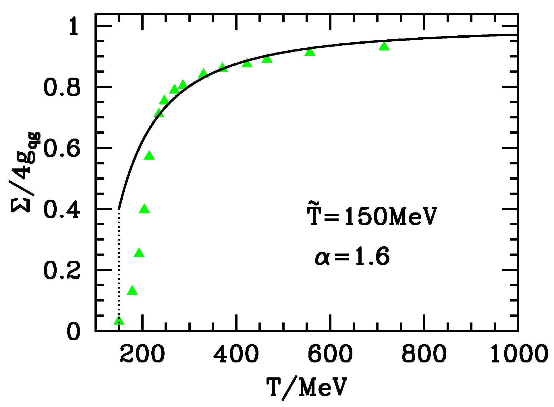
Much work has recently been done to obtain the s.i. matter state equation close to $T_c$. For a recent review, see, e.g., [28]. In Figure 1 of this paper, various outputs of lattice computations are considered. In the sequel, we shall mostly use “$p4(N_{\tau }=6)$” outputs, due to these being those that extend to the greatest value of T. In Figure 2, green triangles report lattice outputs compared with the second expression (6) for $\tilde{T}=150$ MeV and $\alpha =1.6$. The fit can be improved if more decimals are allowed, but, even so, the figure shows that expression (6) is able to meet the 10 highest–T points; although purely phenomenological, such an expression surely performs better than perturbative expression or expressions tentatively including non perturbative effects by introducing suitable mass scales and/or making recourse to effective descriptions (see, e.g., [29,30]; references related to different attempts can also be found in [31].

Let us also add that a fit of the generalized bag–model to the “$p4(N_{\tau }=8)$” leads to $\tilde{T}\simeq 160$ MeV and $\alpha \simeq 1.5$; results do not appear so impressive because the region of the two highest–T “green” points is not covered, but the comparison between $\tilde{T}$ and α values used gives us an idea of the actual uncertainty on fitting parameters. Let us add that $asqtad$ outputs are not so far from $p4$ results, but concern a lower T range, where we cannot claim expression (6) to apply. Altogether, expressions (5) and (6) appear suitable to fit only higher T points, although in a fairly wide range. On the contrary, in the region of the five lowest-T “green” points, expressions (5) and (6) are far from lattice data. In Figure 2, the plot of the analytical curve is, however, terminated at $T=\tilde{T}$; below such a temperature, expression (5) would return a negative pressure.

Let us now outline how we intend to interpret the fit to these data. The region where the fit nicely meets green points should account for a gradual passage from QG plasma to a gas of confined hadrons. The sixth green point region (from low T), below which the fit no longer works so nicely, locates crossover completion: at lower T, no free quarks remain; since then, confinement forces act only inside hadrons. Accordingly, at smaller temperatures, the density can decrease quickly, and fits could only be attempted, perhaps, with expression based on hadron behavior, as those considered by [26].

However, within such a context, the analytic curve does not totally loose significance even in the low-T region. It could be interpreted as an upper limit to the entropy content in s.i. matter form at such T, still allowing for a fluid where quarks (confined or unconfined), however, lay at distances $<\sim T_c^{-1}$, so that gluons arising from residual free quarks can still be reabsorbed “in time”. This would be the region of mild violations of the equilibrium entropy sharing among cosmic components, possibly required by the persistence of B carrying free quarks. On the contrary, once attaining a negative pressure, we approach a regime where a sort of mini-inflation would occur, with creation of quark–antiquark pairs by confinement forces, so that the overall quark number density does not shift below a limiting value. This would be the region of strong violations.

Of course, all of this is just a tentative modeling for situations still out from full numerical control. However, it lends us a tool to model what happen in the case of delayed baryon formation, according to the value of the abovementioned parameter f.

We believe that suitable lattice computations can provide f-values with a fair approximation. Being still unavailable, we shall consider here the reasonably worst option: that cosmic evolution occurs along the analytical curve until $p=0$. By then, the B transfer is completed, so that no mini-inflation and entropy input occur, while the following expansion takes place with a rapid transformation of s.i. matter entropy into photon–lepton entropy. For what concerns cosmic evolution, this is similar to what was found to occur in a first order phase transition occurring exactly at $T_c$ and, therefore, without entropy input. The above expressions (5) and (6) will then enable us to integrate cosmic expansion equations during such an epoch.

In the next section, we shall reconsider such problems in the frame of SCDEW cosmologies.

3. An Analytical Description of the Cosmological QH Transition, and Coupled DM-DE Equilibrium Recovery in SCDEW Models

Wishing now to consider the transition within a cosmological context, let us recall the cosmic background metric if (almost) flat, even today, while the density parameter of matter (baryons plus DM) is ${\mathsf{\Omega }}_m\simeq 0.3$; detailed values can be found, e.g., in the recent report of the Planck collaboration [32]. This suggests the existence of a component or phenomenon, denominated as DE, filling the gap. To be also consistent with SNIa data (see, e.g., [33]), it should also cause cosmic expansion to accelerate.

The ΛCDM model, initially revived to meet acceleration data, has then become a sort of standard cosmology, not only because it fulfills the above requirements, but also for meeting much more data well beyond cosmological acceleration and background composition, which can be suitably accommodated inside it. However, such a model, assuming that DE has a state equation $p=w\rho$ with $w\equiv -1$ ($p,\rho$: average cosmic pressure and energy density), implies a mess of paradoxes and conundrums, so that it is mostly considered just a sort of effective model, hiding a deeper physical reality that present data are insufficiently detailed to discriminate.

While new experiments are running to enrich the datasets (see, e.g., LSST (http://www.lsst.otg/lsst/) and Euclid [34], much work has been devoted to forge cosmological models, overcoming ΛCDM conundrums while being indistinguishable from it, within the context of available datasets.

3.1. SCDEW Cosmologies

Cosmologies involving Strongly Coupled DM and DE, plus warm DM (SCDEW), are a possible option among them. They start from the discovery of an attractor solution for a Friedman equation in the early radiation-dominated Universe, which, at variance from any other models, involves early non–radiative components. Let us summarise how this works.

The energy density of non-relativistic uninteracting DM and a purely kinetic scalar field Φ, in a radiatively expanding environment, dilute as $a^{-3}$ and $a^{-6}$, respectively. Here, a is the scale factor and

$$d{s}^2=a^2\left(\tau \right)(d{\tau }^2-d{\lambda }^2)$$

(7)

is the background metric, τ and $d\lambda$ being the conformal time and the comoving distance element, respectively. However, if DM and Φ are coupled and energy flows from DM to Φ, both of the above components could be led to dilute as $a^{-4}$, just as background radiation.

This expectation is confirmed by precise calculations, showing that the Lagrangian coupling needed to obtain this result bears a Yukawa-like form

$${\mathcal{L}}_I=-g{m}_{p}exp(-b\mathsf{\Phi }/m_p)\overline{\psi }\psi .$$

(8)

Here: ψ is a spinor field yielding DM; $m_p$ is the Planck mass; and g and b are suitable constants, the former one being subject to loose constraints, while the latter one can be used to define the coupling constant

$$\beta =b\sqrt{3/16\pi }.$$

(9)

It can then be shown that, if DM and Φ have density parameters

$${\mathsf{\Omega }}_c=1/2{\beta }^2\mathrm{and}{\mathsf{\Omega }}_{\mathsf{\Phi }}=1/4{\beta }^2,$$

(10)

the cosmic expansion proceeds along an attractor, i.e., both radiation and the coupled $DM$-Φ component keep stable proportions, all diluting as $a^{-4}$. Notice that all this implies that ${\beta }^2>3/4$, and this is why this approach implies a strong coupling between DM and Φ. Of course, if $\beta \equiv \sqrt{3}/2=0.8660$, there is no room for ordinary radiation. 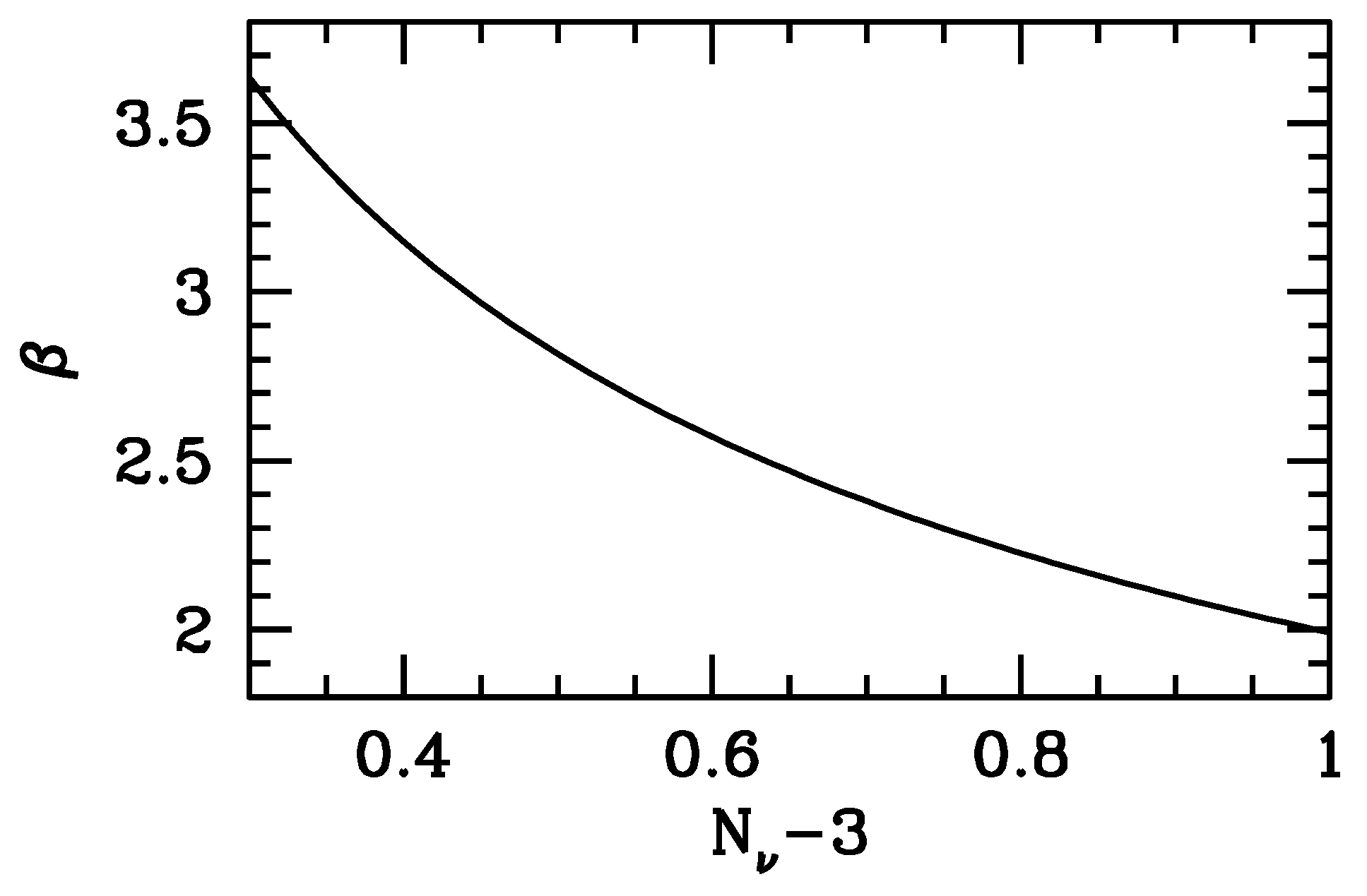At the passage through big–bang nucelosynthesis (BBN) and at the last scattering band (LSB), the coupled $DM$–Φ component is a sort of dark radiation (DR). In Figure 3, we plot the values of β corresponding to a given amount of DR, expressed in terms of extra neutrino species.

BBN is consistent with data even if DR accounts for up to about one extra neutrino species. Accordingly, β values as low as two appear acceptable. A stronger constraint comes from CMB data. As shown by [12], the actual amount of DR has (slightly) increased, at the passage through the LSB, because of the end of the self-similar expansion regime after matter–radiation equivalence. At the LSB, one extra neutrino species corresponds then to $\beta =2.5$. According to [32], at the 95 $\%$ confidence level, the number of extra neutrino species allowed are ≃$0.7$. Taking one extra neutrino species exceeds this limit. However, besides being clearly consistent with data within three σs, such a greater value of $N_{\nu }$ would favor Hubble constant values ∼$0.72$, consistent with direct observations. On the contrary, the best fit of the Planck collaboration data disagrees with them. Therefore, we can set the lower limit to coupling at $\beta =2.5.$

Here below, most results will be shown for $\beta =8$. However, when considering the impact of QH transition on BBN, we shall compare results for $\beta =2.5$ and 10.

Altogether, the dynamical equations derived by the coupling Lagrangian ${\mathcal{L}}_I$ and the kinetic terms can be set in the form

$$\dot{a}={(8\pi /3)}^{1/2}{({\rho }_c+{\rho }_{\mathsf{\Phi }}+{\rho }_r)}^{1/2}a/m_p,$$

$${\dot{\rho }}_c=-3{\rho }_c/\tau -{\rho }_c{\mathsf{\Phi }}_{1}b/m_p,$$

$${\dot{\mathsf{\Phi }}}_1=-2{\mathsf{\Phi }}_1/\tau +{\rho }_c{a}^{2}b/m_p,$$

(11)

provided we assume DM to be fully non–relativistic, its density being ${\rho }_c$. Here, ${\mathsf{\Phi }}_1=\dot{\mathsf{\Phi }}$, dots yielding differentiation in respect to τ, while ${\rho }_r$ is the density of the whole thermal soup. As the decreasing cosmic temperature shifts below the mass value of any particles, the standard event is that they annihilate by keeping a constant value of cosmic entropy

$$S=\frac{4}{3}\frac{{\pi }^2}{30}g{T}^3{a}^3,$$

(12)

even though

$$g={\mathcal{N}}_b+\frac{7}{8}{\mathcal{N}}_f$$

(13)

(${\mathcal{N}}_{b,f}:$ number of independent spin states of bosons, fermions with $m<T$) has decreased. As S is constant, and $\rho =({\pi }^2/30)g{T}^4,$ it shall be

$$\rho \propto g^{-1/3}{a}^{-4},$$

(14)

so that “radiation” deviates from a pure $a^{-4}$ diluting by exhibiting an upward jump due to g decrease.

When this happens, ${\rho }_c$ and ${\rho }_{\mathsf{\Phi }}$ also should shift upward, so that ${\mathsf{\Omega }}_c$ and ${\mathsf{\Omega }}_{\mathsf{\Phi }}$ preserve the values (10). In other terms, the attractor solution, perturbed by g decrease, must rearrange; but the process may take some time and its duration can be tested just by inserting ${\rho }_r$ behavior in Equation (11).

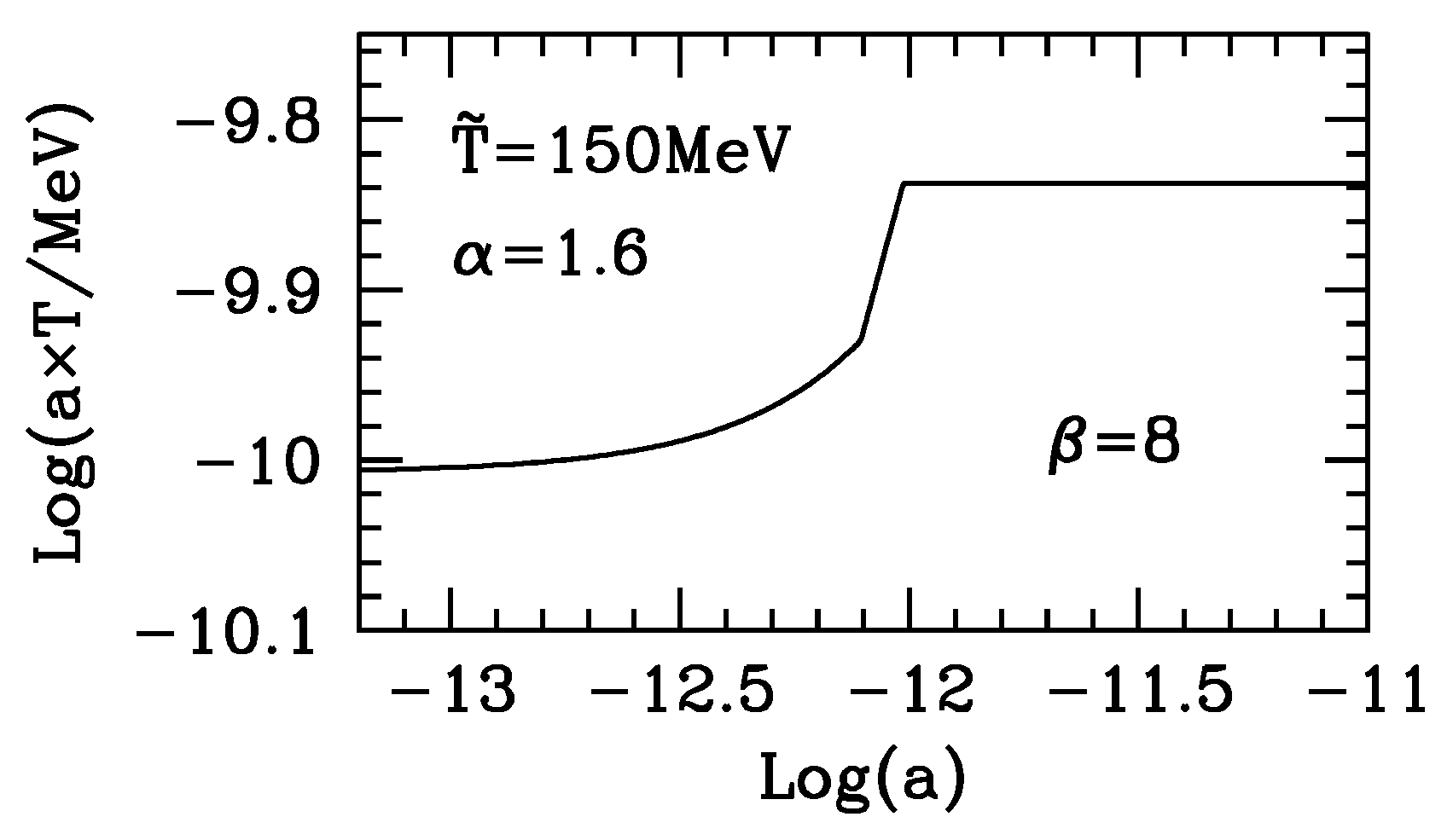
The greatest jump the attractor may then have to face is at the QH transition, when g shall exhibit a drastic decay within quite a short temperature interval. An even more drastic event will occur if the reasonably worst option, considered in the previous section, is true. In this case, the decrease of the effective g shall take place while T stays constant at $\tilde{T}$ along the dashed line in Figure 2.

Before studying the behavior of densities across such a transition, let us briefly complete the reminder on SCDEW cosmologies. The attractor solution for Equation (11) was found by Bonometto et al. (2011), who also studied the behavior of cosmic components at lower Ts, showing that it easily meets the observed proportions of background components. Of course, this requires that the Φ field shifts from kinetic to potential at a suitable time. This can be obtained without making recourse to a specific (tracker) potential, as detailed in the above paper. Bonometto and Mainini [35] then studied the evolution of density fluctuations within such cosmologies, finding that CMB anisotropies and polarization are substantially indistinguishable from ΛCDM and calculating the linear transfer function. More recently, Macció et al. [13] performed N-body simulations for some model versions, finding that it reproduces ΛCDM findings at scales above average galaxy sizes, while substantially easing long standing ΛCDM problems such as dwarf galaxy profiles, MW satellites, and galaxy concentration distribution.

Altogether, all nice ΛCDM outputs are practically overlapped by SCDEW, which, however, allows the abovementioned improvements over lower scales while eradicating all conceptual problems going with a simple-minded ΛCDM scheme. A number of subtle tests can, however, be devised, enabling us to distinguish between SCDEW and ΛCDM. As expected, they shall be possible only when a much higher level of precision will be attained by observations. It is also fair to outline that SCDEW involves a number of extra parameters, but no fine tuning is needed for any of them. A final point is that the Lagrangian ${\mathcal{L}}_I$ could also account for post-inflationary reheating and the field Φ, besides of beind today’s DE, could also play an important role in the inflationary process.

3.2. Attractor Behavior at the Cosmological QH Transition

Taking into account expressions (4) and (6), we find that, in the proximity of the QH transition, the ${\rho }_r$ term at the r.h.s. of the first Equation (11) shall read

$${\rho }_r=\frac{{\pi }^2}{30}\left\{g_{\gamma ,lep}+g_{ql}\left[1-\left(1-\frac{\alpha }{3}\right){\left(\frac{\tilde{T}}{T}\right)}^{\alpha }\right]\right\}{T}^4(\mathrm{for}T>\tilde{T}\mathrm{and}a<a_1),$$

$${\rho }_r=\frac{{\pi }^2}{90}\left[\left(4g_{\gamma ,lep}+\alpha g_{ql}\right){\left(\frac{a_1}{a}\right)}^3-g_{\gamma ,lep}\right]{\tilde{T}}^4(\mathrm{for}T\equiv \tilde{T}\mathrm{and}{a}_1<a<a_2),$$

$${\rho }_r=\frac{{\pi }^2}{90}{g}_{\gamma ,lep}{T}^4(\mathrm{for}T<\tilde{T}\mathrm{and}a>a_2).$$

(15)

Here, $g_{\gamma ,lep}$ is the statistical weight of lepton–photon spin states. Amongst leptons, we also include μ particles; their progressive annihilation, when $T<m_{\mu }$, will be disregarded, in order not to confuse its effects of QH transition.

Owing to S conservation before, during, and after the transition, the scale factor at its end shall be

$$a_2=\frac{T_0}{\tilde{T}}{a}_0\times {\left(\frac{g_0}{g_{\gamma ,lep}}\right)}^{1/3},\mathrm{with}{g}_0=2(1+2.625/{2.75}^{4/3}),$$

(16)

accounting for the effective number of spin states at the present cosmic temperature $T_0$ (scale factor $a_0$) by assuming three (∼massless) neutrino flavors. This scale factor is reached after a temperature plateau (at $\tilde{T}$), starting when the scale factor is

$$a_1=a_2{\left(\frac{g_{\gamma ,lep}}{g_{\gamma ,lep}+g_{qg}/4}\right)}^{1/3}.$$

(17)

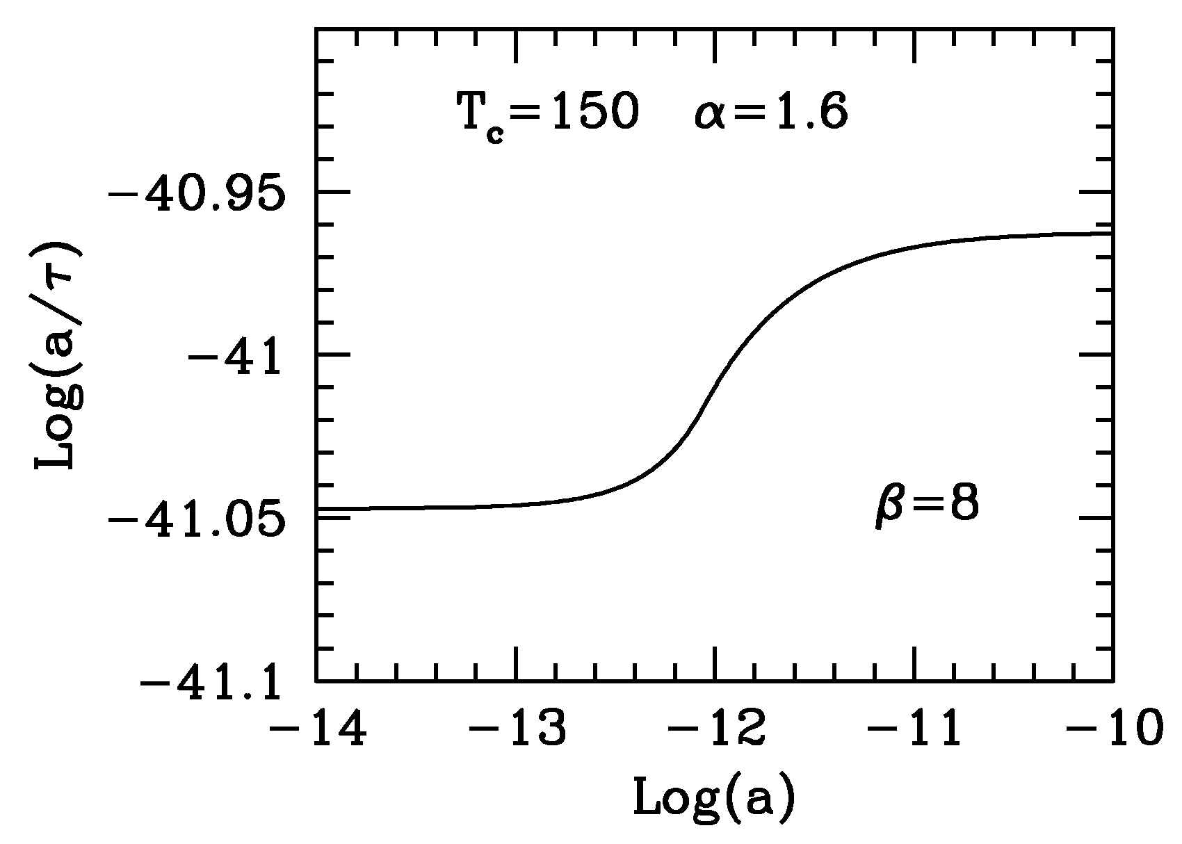
Of course, as soon as ${(\tilde{T}/T)}^{\alpha }$ acquires a significant value (in comparison with unity), the standard cosmological behavior $aT=\mathrm{const}.$ is violated. In Figure 4, we show the size of such a violation for $\alpha =1.6$ and compare it with the case $\alpha =2$. This behavior is obtainable just from S conservation and is only mildly dependent on β, provided it is not too close to its lower limit $\sqrt{3}/2$. The plot was obtained, however, for $\beta =8,$ as all plots here below.

In particular, in Figure 5, the same effect is seen in more detail all through the transition. When hadrons become substantially negligible, $aT$ recovers a fully constant behavior vs. a.

During a radiative expansion, when $\rho a^4=\mathrm{const}.$, the Friedman eq. reads

$$\frac{1}{{\tau }^2}=\frac{8\pi }{3m_p^2}\rho a^2\propto \frac{1}{a^2},$$

(18)

so that $a\propto \tau$. When $\rho a^4$ is no longer constant, as during the QH transition, this proportionality can be violated. In Figure 6, we show such violations through QH transition.

3.3. Density Anomalies Caused by QH Transition

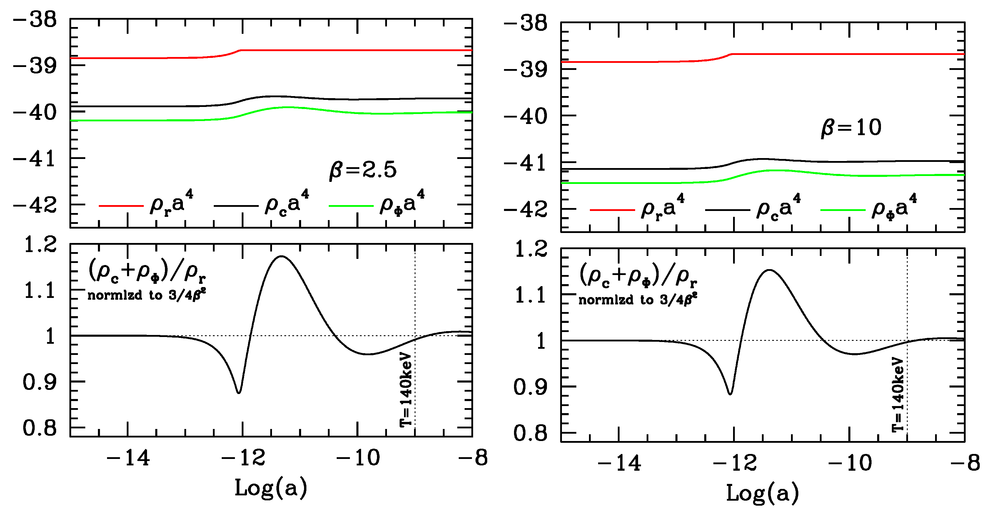
Let us finally discuss the effects of QH transition on early ${\mathsf{\Omega }}_c$ and ${\mathsf{\Omega }}_{\mathsf{\Phi }}$ values. QH transition is likely to be the greatest push out of the attractor solution that cosmic components receive during early expansion. It is shown in Figure 7 both for $\beta =2.5$ and $\beta =10.$

The initial effect of the transition is to decrease the ratio $({\rho }_c+{\rho }_{\mathsf{\Phi }})/{\rho }_r$ by ∼$12\%$, almost independently of β, showing that the increase of radiation density, at QH transition, is only partially followed by coupled DM and Φ densities. The subsequent rebounce upward, however, is wider, its amount being slightly greater for smaller β values, and occurs when the temperature has already lowered to T∼ 20 MeV.

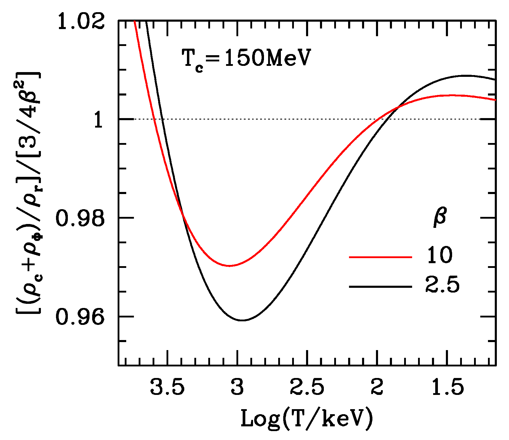
Residual perturbations at the eve of BBN depend still more on β and can be better appreciated in Figure 8. Just at the time of neutrino decoupling (∼900 keV), we have a second minimum. The fraction of cosmic materials in the radiative component is then almost steadily increasing until the reaching of deuterium bottleneck.

In general, the possible impact on BBN is obviously greater for lower β. However, even for $\beta =2.5$, the coupled DM–Φ component has a limited impact on the overall density, approximately equivalent to a half extra neutrino species, seemingly consistent with primeval abundance limits. On top of that, we have residual ${\rho }_r/{\rho }_{total}$ oscillations, so that the scale dependence of both overall and radiation expansions exhibit incoherent discrepancies in respect to a purely radiative regime. For $\beta =2.5$, discrepancies can be $\mathcal{O}(0.5\%)$ and almost steadily continue all through the period going from ν-decoupling to the synthesis of ${}^{2}H$ and other nuclides. Quantitatively, such deviation is not much less than half of what is due to electron–positron annihilation.

Of course, no major changes in BBN predictions can be expected because of these density shifts. The point is that, knowningly, this kind of deviation from the standard model were never tested in BBN numerical experiments. Even though such variations are mild, however, they would be a signature of SCDEW models in respect to ΛCDM.

In general, discrepancies between SCDEW and ΛCDM results are mild. This is a SCDEW peculiarity and a major merit. In fact, no other variations within the frame of available data is appreciable. A final word on variations in the estimated light nuclide abundances, arising from such slight deviations from a ΛCDM-like expansion regime, can hardly be said without direct inspection. It is not unreasonable to expect that this effect is also rather small, but this is the kind of discrepancy that may enable us to say a final word on SCDEW being the true underlying cosmology yielding an apparent ΛCDM.

4. Discussion

The Universe arrives at the QH transition with a tiny excess of quarks, in respect to anti-quarks. On average, then, in any volume with ∼1000 (anti)quarks across, there is one extra quark carrying B. As the direct formation of quark triplets is a rare process, when most quark–antiquark pairs undergo mutual annihilation into photon–letpon pairs, in order to transfer B from the QG plasma to the hadronic gas, we should probably rely on the formation of diquark couples, aside from the straight quark–antiquark proto-hadrons, when the transition has a start; i.e., statistical equilibrium should prescribe that a sufficient fraction of quarks enter homo rather than hetero couples at the beginning of the transition. Then, baryons can form through ordinary two-body collisions between quark and diquark, provided that the center-of-mass energy is sufficiently high and there is correct color matching. We estimated that the minimal requirement to allow this to happen is that the fraction f of quarks embedded in diquarks at the beginning of the QH transition is not less than $1:{10}^6$.

This, however, pushes us to consider the possibility that, until B has not fully transferred from QG plasma to hadron gas, s.i. materials could not dilute to densities significantly <$T_c^3$, in order to maintain mutual inter-quark distances ∼$T_c^{-1}$. This requirement could cause a deviation of s.i. matter and entropy densities (${\rho }_{qg}$ and ${\sigma }_{qg}$) from straightforward lattice predictions.

Lattice computation shows that the inter-quark distance gradually increases at the approaching of a suitable temperature $T_c$, in order to then undergo a faster decrease about such $T_c$. We showed that the expressions

$${\rho }_{qg}=\frac{{\pi }^2}{30}{g}_{qg}\left[1-(1-\frac{\alpha }{3}){\left(\frac{\tilde{T}}{T}\right)}^{\alpha }\right]T^4,{\sigma }_{qg}=4\frac{{\pi }^2}{90}{g}_{qg}\left[1-(1-\frac{\alpha }{4}){\left(\frac{\tilde{T}}{T}\right)}^{\alpha }\right]T^3,$$

(19)

for energy and entropy density, provide a fair fit to higher–T lattice outputs with $\alpha =1.5$–1.6 and $\tilde{T}\sim 150$ MeV. These expressions are a generalization of the old MIT bag model, which is obtained again if $\alpha =4$. They, however, cease to meet lattice results in the fast decreasing regions. In turn, the related pressure expression

$$p_{qg}=\frac{{\pi }^2}{90}{g}_{qg}\left[1-{\left(\frac{\tilde{T}}{T}\right)}^{\alpha }\right]T^4,$$

(20)

yields a faster decrease of pressure p, implying a negative pressure at $T<\tilde{T}$.

It should be outlined that this somehow strengthens the significance of expressions (19) and (20). In the cosmological context, a negative pressure could lead to a sort of mini-inflation—s.i. matter being produced by confinement forces, rather than allowing for a plasma with mutual particle distances ≫$T_c^{-1}$. However, even without considering such an extreme option in the temperature interval between $T_c$ and $\tilde{T}$, these expressions are still useful to model equilibrium deviations if and when B-transfer is delayed. This is what we did in this work in order to estimate the cosmological effects of a possible diquark fraction $f<{10}^{-6}$.

In more detail, we considered a specific example of the transition being delayed just until $\tilde{T}$ is reached, considering it as the worst reasonable option. Then, in the frame of SCDEW models, the delay yields significant oscillations in the ratio between radiative materials and the coupled DM-Φ component. We provide a numerical solution of the three-equation system yielding these oscillations, showing that they may propagate down to BBN.

We then showed that we can expect a (mild) deviation from a purely radiative expansion between neutrino annihilation and ${}^{2}H$ synthesis. Quantitatively, it can reach half of the deviation due to electron–positron annihilation. However, to our knowledge, such a kind of deviation from standard ΛCDM models was never numerically tested.

Readers should be reminded, however, that, at present, no available data allow us to discriminate between SCDEW and ΛCDM, the main merit of SCDEW being its capacity to faithfully reproduce ΛCDM data by avoiding its conceptual problems while also relating the inflationary field with DE (as a matter of fact, SCDEW also eases some ΛCDM problems below the galactic scale; Macció et al. [13]).

It is therefore important to devise the areas where more refined data could allow us to finally discriminate between these two sets of cosmologies. In this paper, we outlined that QH transition could be entangled with finding one such area.

5. Conclusions

In summary, we are led to ask QCD specialists and BBN cosmologists two separate questions: (i) is it possible to provide a really reliable estimate of the fraction of quarks in diquark couples along the crossover transition? (ii)electron–positron annihilation causes a deviation from radiative matter dilution $\propto a^{-4}$ during BBN. How much smaller can a further deviation be during the same period in order to be appreciable through observational light nuclide abundances? As a matter of fact, we can expect that the QH transition causes an echo extending down to BBN, with significant deviations from radiative matter dilution $\propto a^{-4}$, ranging between 1/4 and 1/2 of what is due to electron–positron annihilation.