Starobinsky-Like Inflation and Running Vacuum in the Context of Supergravity

Abstract

We describe the primeval inflationary phase of the early Universe within a quantum field theoretical (QFT) framework that can be viewed as the effective action of vacuum decay in the early times. Interestingly enough, the model accounts for the “graceful exit” of the inflationary phase into the standard radiation regime. The underlying QFT framework considered here is supergravity (SUGRA), more specifically an existing formulation in which the Starobinsky-type inflation (de Sitter background) emerges from the quantum corrections to the effective action after integrating out the gravitino fields in their (dynamically induced) massive phase. We also demonstrate that the structure of the effective action in this model is consistent with the generic idea of re-normalization group (RG) running of the cosmological parameters; specifically, it follows from the corresponding RG equation for the vacuum energy density as a function of the Hubble rate, ${\rho }_{\Lambda }\left(H\right)$. Overall, our combined approach amounts to a concrete-model realization of inflation triggered by vacuum decay in a fundamental physics context, which, as it turns out, can also be extended for the remaining epochs of the cosmological evolution until the current dark energy era.

1. Introduction

In the last two years, we have witnessed extraordinary developments on experimental tests of inflationary models [1], based on studies of photons in the Cosmic Microwave Background radiation. In particular, the results of Planck collaboration [2,3,4] and the associated non-observation of B-mode polarizations of primordial light fluctuations have imposed very stringent restrictions on single scalar-field models of slow-roll inflation, allowing basically models with a very low tensor-to-scalar fluctuation ratio $r=n_T/n_s\ll 1$, with a scalar spectral index $n_s\simeq 0.96$ and no appreciable running. In fact, the upper bound set by Planck collaboration [2,3,4] on this ratio, as a consequence of the non-observation of B-modes, is $r<0.11$, but their favoured regions point towards $r\le {10}^{-3}$. This is a feature that characterizes the so-called Starobinsky-type (or $R^2$-inflation, with R denoting the scalar spacetime curvature) inflationary models [5]. The estimated energy scale $E_I$ of inflation, which in inflaton-type models is related to the, approximately constant, scalar potential during inflation through $E_I=V_I^{1/4}$, reads [1]:

$$E_I={\left(3H_I^2{M}_{\mathrm{Pl}}^2\right)}^{1/4}\simeq 2.1\times {10}^{16}\times {\left(\frac{r}{0.20}\right)}^{1/4}\mathrm{GeV},$$

(1)

where $M_{\mathrm{Pl}}=1/\sqrt{8\pi G}\simeq 2.43\times {10}^{18}\mathrm{GeV}$ is the reduced Planck mass (G being the Newtonian constant). The upper bound $r<0.11$ placed by the Planck collaboration implies:

$$H_I=1.05{\left(\frac{r}{0.20}\right)}^{1/2}\times {10}^{14}\mathrm{GeV}\le 0.78\times {10}^{14}\mathrm{GeV}.$$

(2)

The above can be rephrased as $H_I/m_P⩽6.39\times {10}^{-6}$, where $m_P=1/G^{1/2}=\sqrt{8\pi }{M}_{\mathrm{Pl}}\simeq 1.22\times {10}^{19}$ GeV is the Planck mass in natural units. This result is consistent with the well-known CMB bound $H_I/m_P\lesssim {10}^{-5}$ on the temperature fluctuations induced by the tensor modes. As we will see, the actual value of H during inflation for the class of models under study satisfies $H\lesssim H_I$, and hence, the CMB bound is preserved by them.

The recent joint BICEP2-Planck analysis [6] confirmed the early Planck result, namely the likelihood curve for r yields an upper limit $r<0.12$ at $95\%$. Moreover, the present BICEP2-Planck data are consistent with a scalar spectral index $n_s\simeq 0.96$ and no appreciable running, in agreement with the previous Planck data [2,3,4]. Using the aforementioned new upper limit $r_{\max }=0.12$, the Hubble parameter during slow-roll inflation $H_I$ is estimated to be below:

$$H_I^{\mathrm{Bicep}2+\mathrm{Planck}}\le 0.81\times {10}^{14}\mathrm{GeV},$$

(3)

and hence, $H_I/m_P⩽6.64\times {10}^{-6}$. Because of the low significance of the new limit on r, the possibility that r is actually much smaller than the current upper limit $r_{\max }$ remains as natural as it was before. In fact, nothing actually prevents at present that the typical value of the tensor to scalar ratio can be, for example, $r=\mathcal{O}\left({10}^{-3}\right)$, and in this sense, the Starobinsky-type scenarios can still be considered as a serious possibility to describe the inflationary Universe. Following this point of view, we continue in this paper with the investigation of Starobinsky-like models as potential candidates for the realistic implementation of inflation compatible with the data.

In previous publications one of us (Nick E. Mavromatos) with collaborators [7,8] discussed the dynamical breaking of supergravity (SUGRA) theories via gravitino condensation and demonstrated [9] the compatibility of this scenario with Starobinsky-like [5] inflationary scenarios. As we discussed, this phase is characterized by the dynamical emergence of a de Sitter background. As argued in [7,8], the Starobinsky-type inflation appears much more natural (from the point of view of the order of the parameters involved) than a hill-top inflation scenario [10] in which the gravitino condensate itself is the inflaton field. In the latter, very large values of the wave function re-normalization of the condensate field are required to ensure slow-roll inflation if one insists on (phenomenologically realistic) sub-Planckian supersymmetry breaking scales. It is important to notice at this point that in the original Starobinsky model [5], the $R^2$ terms crucial for inflation arise from the conformal anomaly in the path integral of massless (conformal) matter in a de Sitter background, and thus, their coefficient is arbitrary and can only be fixed phenomenologically. A similar, although not identical, situation occurs in the context of anomaly-induced inflation [11,12,13], where the term $R^2$ is absent at the classical level, but is generated from the conformal anomaly. In this case, however, the coefficient of $\square R$ (entering the β-functions and controlling the stability of inflation) presents also some arbitrariness, which can only be fixed by a special re-normalization condition. Par contrast, in the considered SUGRA scenario, such terms arise in the one-loop effective action of the gravitino condensate field, evaluated in a de Sitter background, after integrating out massive gravitino fields, whose mass was generated dynamically. The order of the de Sitter cosmological constant, $\Lambda >0$, that breaks supersymmetry and the gravitino mass are all evaluated dynamically (self-consistently) in our approach from the minimization of the effective potential. Thus, the resulting $R^2$ coefficient, which determines the phenomenology of the inflationary phase, is calculable [9].

Also very important for our considerations is the framework of the running vacuum model (RVM) [13,14,15,16,17,18,19]; see [20,21,22] and the references therein for a recent detailed exposition. The implications of these dynamical vacuum models have recently been analysed both for the early Universe [22,23,24,25,26,27,28], as well as for the phenomenology of the current Universe [29,30,31]; see also [32,33,34,35,36,37,38,39,40] for previous analyses.

In regard to the early Universe, we emphasize that the RVM defines a class of non-singular inflationary scenarios with graceful exit into the standard radiation regime. These models are related to Starobinsky inflation models, although they are not equivalent. We will discuss in this paper the correspondence between them and most particularly with the dynamically-broken SUGRA model with gravitino condensation that we have mentioned above. It is especially remarkable that such a specific implementation of the SUGRA model leads, as we will show in this paper, to the effective behaviour of the RVM with calculable coefficients. In this way, the former automatically benefits from the successful consequences of the latter. Let us mention that the RVM also provides some important clues for alleviating the cosmological constant problem [20,21].

Finally, we would like to mention that the RVMs have been tested against the wealth of accurate SNIa + BAO + $H\left(z\right)$ + LSS + BBN + CMB data (see [41] for a recent summary review), and they turn out to provide a quality fit that is significantly better than the ΛCDM. This fact has become especially prominent in light of the most recent works [42,43]. Therefore, there is every motivation for further investigating these dynamical vacuum models from different perspectives, with the hope of finding possible connections with fundamental aspects of the cosmic evolution. In point of fact, this is the main aim of this work.

The structure of the article is as follows. The general framework of the RVM is introduced in Section 2. The basic theoretical elements of the Starobinsky inflation are presented in Section 3. The main properties of the dynamical breaking of local SUGRA theory and its connection to Starobinsky-type inflation are reviewed in Section 4. In Section 5, we demonstrate how the RVM describes the effective framework of the Starobinsky [5] and the dynamically-broken SUGRA [10] models at the inflationary epoch. Finally, our conclusions are summarized in Section 6.

2. Running Vacuum: A Natural Arena for Vacuum Decay in Cosmology

It is the purpose of this work to go one step further from demonstrating the compatibility of the dynamically-broken SUGRA scenario [7,8,9] with inflation and to discuss the possibility of a dynamical evolution of the inflationary phase ground state to the standard radiation regime within the context of the running vacuum model (RVM) of the cosmic evolution utilizing an effective “re-normalization group (RG) approach”; see [13,14,15] and [20,21,22] for comprehensive expositions. Specifically, we wish to show that the behaviour of the aforementioned SUGRA scenario effectively mimics the RVM. Once this link is elucidated, the general “decaying” vacuum description inherent to the RVM formulation allows one to smoothly connect inflation to the standard Fridman–Lemaître–Robertson–Walker (FLRW) radiation era, which subsequently proceeds into a matter and dark energy domination in the present era, in which it still carries a mild dynamical behaviour compatible with the current cosmological data [29,30]. Such an expansion history of the Universe has been put forward in previous works by the authors in various collaborations and contexts, e.g., non-equilibrium string-inspired cosmologies [44,45,46] or conventional field-theoretic cosmologies in which the above-mentioned RVM is extensively applied for the study of the early cosmic history [23,24,25,26,28].

In the effective RG approach underlying the RVM, one can write down an evolution equation for the effective vacuum energy density ${\rho }_{\Lambda }\left(t\right)={\rho }_{\Lambda }\left({\mu }_c\left(t\right)\right)$, treated as a dynamical quantity whose cosmic time evolution is inherited from its dependence on a characteristic cosmic scale variable ${\mu }_c={\mu }_c\left(t\right)$. This variable plays the role of the running (mass) scale of the re-normalization group approach, and a natural candidate for such a scale in FLRW cosmology is the Hubble parameter $H\left(t\right)$. Therefore, the proposed RG equation is [20,21]:

$$\frac{d{\rho }_{\Lambda }\left(t\right)}{d\ln H^2}=\frac{1}{{\left(4\pi \right)}^2}\sum _i\left[a_i{M}_i^2{H}^2+b_i{H}^4+c_i\frac{H^6}{M_i^2}+\cdots \right].$$

(4)

In general, ${\mu }_c^2$ can be associated with a linear combination of $H^2$ and $\dot{H}$, and the variety of terms appearing on the r.h.s. of (4) can be richer [22]; however, the canonical possibility is the previous one, and hereafter, we restrict to it. The coefficients $a_i,b_i,c_i\cdots$ appearing in (4) are dimensionless and receive contributions from loop corrections of boson and fermion matter fields with different masses $M_i$. It must be stressed that the general covariance of the action [13,16,17,18,19] necessitates the appearance of only even powers of the (cosmic-time t dependent) Hubble parameter $H\left(t\right)$ on the right-hand-side of (4). For a specific framework where the above RG is concretely realized and the β-function coefficients can be computed, see [13].

We note at this stage that, if the evolution of the Universe is restricted to eras below the grand unified theory (GUT) scale, then for all practical purposes, it is at most the $H^4$ terms (those with dimensionless coefficients $b_i$) that can contribute significantly. The $H^2$ term is of course negligible at this point, and the higher powers of $H^n$ for $n=6,8,..$ are suppressed by the corresponding inverse powers of the heavy masses $M_i$, which go to the denominator, as required by the decoupling theorem. In the scenarios of the dynamical breaking of local supergravity discussed in [7,8,9,10], the breaking and the associated inflationary scenarios could occur around the GUT scale, in agreement with the inflationary phenomenology suggested by the Planck satellite data [2,3,4], provided Jordan-frame supergravity models (with broken conformal symmetry) are used, in which the conformal frame function acquired, via appropriate dynamics, some non-trivial vacuum expectation value. For these situations, therefore, corrections in (4) involving higher powers than $H^4$ will be ignored.

In the next sections, after revising the general framework of Starobinsky inflation, we shall compute ${\rho }_{\Lambda }$ in such supergravity models and study their evolution from the exit from the Starobinsky inflationary phase that occurs in the massive gravitino phase until today. The computation of ${\rho }_{\Lambda }$ will be made via the corresponding calculation of the one-loop effective action after massive gravitinos are integrated out in a path integral. Then, an identification of the effective equation of state can be derived by integrating (4), following the approach of [23,24,25,26,28]. Before doing so, it is instructive to review first the emergence of Starobinsky-type inflation.

3. Generic Starobinsky Inflation

Starobinsky inflation is the oldest model of inflation [5], prior to the traditional, scalar-field-based, inflaton models. It is characterized for being able to realize the de Sitter (inflationary) phase from the gravitational field equations derived from a four-dimensional action that includes higher curvature terms, specifically of the type involving the quadratic curvature correction $\sim R^2$ [5]:

$$\begin{array}{c}\hfill \mathcal{S}=\frac{1}{2{\kappa }^2}\int d^{4}x\sqrt{-g}\left(R+\beta R^2\right),\beta \equiv \frac{8\pi }{3{\mathcal{M}}^2}.\end{array}$$

(5)

Our metric signature is $(-,+,+,+)$, and the definitions of the Ricci and Riemann curvature tensors are $R_{\mu \nu }=R_{\mu \lambda \nu }^{\lambda }$ and $R_{\mu \nu \rho }^{\lambda }={\partial }_{\nu }{\Gamma }_{\mu \rho }^{\lambda }-\cdots$, respectively, i.e., we follow the exact three-sign conventions $(+,+,+)$ of Misner–Thorn–Wheeler [47]).

In the above equation, ${\kappa }^2=8\pi G=1/M_{\mathrm{Pl}}^2$ (in the units of $\hslash =c=1$ we are working on), $\mathrm{G}=1/m_P^2$ is Newton’s (gravitational) constant in four spacetime dimensions, with $m_P$ the Planck mass, and $\mathcal{M}$ is a constant of mass dimension one, characteristic of the model. Notice that the curvature terms in the action are just the dimension-four combination $m_P^{2}R/16\pi +R^2{m}_P^2/\left(6{\mathcal{M}}^2\right)$. With this normalization, $\mathcal{M}$ gives the value of the so-called scalaron mass. The smaller is $\mathcal{M}$ in Planck mass units (i.e., the larger is the dimensionless parameter $m_P^2/{\mathcal{M}}^2$ in front of $R^2$), the longer is the inflationary time (cf. Figure 2 of [22]). Of course, $\mathcal{M}$ cannot be much below the natural scale of inflation, and in fact, it should be of the same order, i.e., $\mathcal{M}\sim M_X$, where $M_X$ is some GUT scale below the Planck mass. Typically, $M_X\sim {10}^{16}\mathrm{GeV}\sim {10}^{-3}{m}_P$.

The most relevant feature of this model is that inflationary dynamics is driven by the purely gravitational sector, through the $R^2$ terms. From a microscopic point of view, these terms can be viewed as the result of quantum fluctuations (at one-loop level) of conformal (massless or high energy) matter fields of various spins, which have been integrated out in the relevant path integral in a curved background spacetime [48,49,50]. The model in fact is to be understood in the context of QFT in curved spacetime. The quantum mechanics of this model, by means of tunnelling of the Universe from a state of “nothing” to the inflationary phase of [5], has been discussed in detail in [51]. The above considerations necessitate truncation to one-loop quantum order and to curvature-square (four-derivative) terms, which implies that there must be a region of validity for curvature invariants, such that $\mathcal{O}\left(R^2/m_P^4\right)\ll 1$. Recalling that $R\sim 12H_I^2$ in the inflationary phase (where $H_I$ is the nearly constant Hubble rate in that phase), we observe that this is indeed a condition satisfied in phenomenologically-realistic scenarios of inflation [1,2], for which the inflationary Hubble scale $H_I$ is typically constrained to obey (2) (Planck data [2,3,4]) or (3) (BICEP2 data), which are at present essentially the same.

Although the inflation in this model is not driven by fundamental rolling scalar fields, nevertheless, the model (5) (and for that matter, any other model where the Einstein–Hilbert spacetime Lagrangian density is replaced by an arbitrary function $f\left(R\right)$ of the scalar curvature) is conformally equivalent to that of an ordinary Einstein-gravity coupled to a scalar field with a potential that drives inflation [52,53]. To see this, one firstly linearises the $R^2$ terms in (5) by means of an auxiliary (Lagrange-multiplier) field $\tilde{\alpha }\left(x\right)$, before rescaling the metric by a conformal transformation and redefining the scalar field (so that the final theory acquires canonically-normalised Einstein and scalar-field terms):

$$\begin{array}{c}{g}_{\mu \nu }\to g_{\mu \nu }^E=\left(1+2\beta \tilde{\alpha }\left(x\right)\right)g_{\mu \nu },\hfill \\ \tilde{\alpha }\left(x\right)\to \kappa \phi \left(x\right)\equiv \sqrt{\frac{3}{2}}\ln \left(1+2\beta \tilde{\alpha }\left(x\right)\right),\hfill \end{array}$$

(6)

where again, $\kappa =\sqrt{8\pi G}$. These steps may be understood schematically via:

$$\begin{array}{c}\int d^{4}x\sqrt{-g}\left(R+\beta R^2\right)\hfill \\ \hookrightarrow \int d^{4}x\sqrt{-g}\left(\left(1+2\beta \tilde{\alpha }\left(x\right)\right)R-\beta {\tilde{\alpha }\left(x\right)}^2\right)\hfill \\ \hookrightarrow \int d^{4}x\sqrt{-g^E}\left(R^E-g^{E\mu \nu }{\partial }_{\mu }\phi {\partial }_{\nu }\phi -V\left(\phi \right)\right),\hfill \end{array}$$

(7)

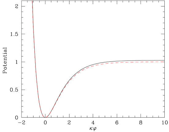
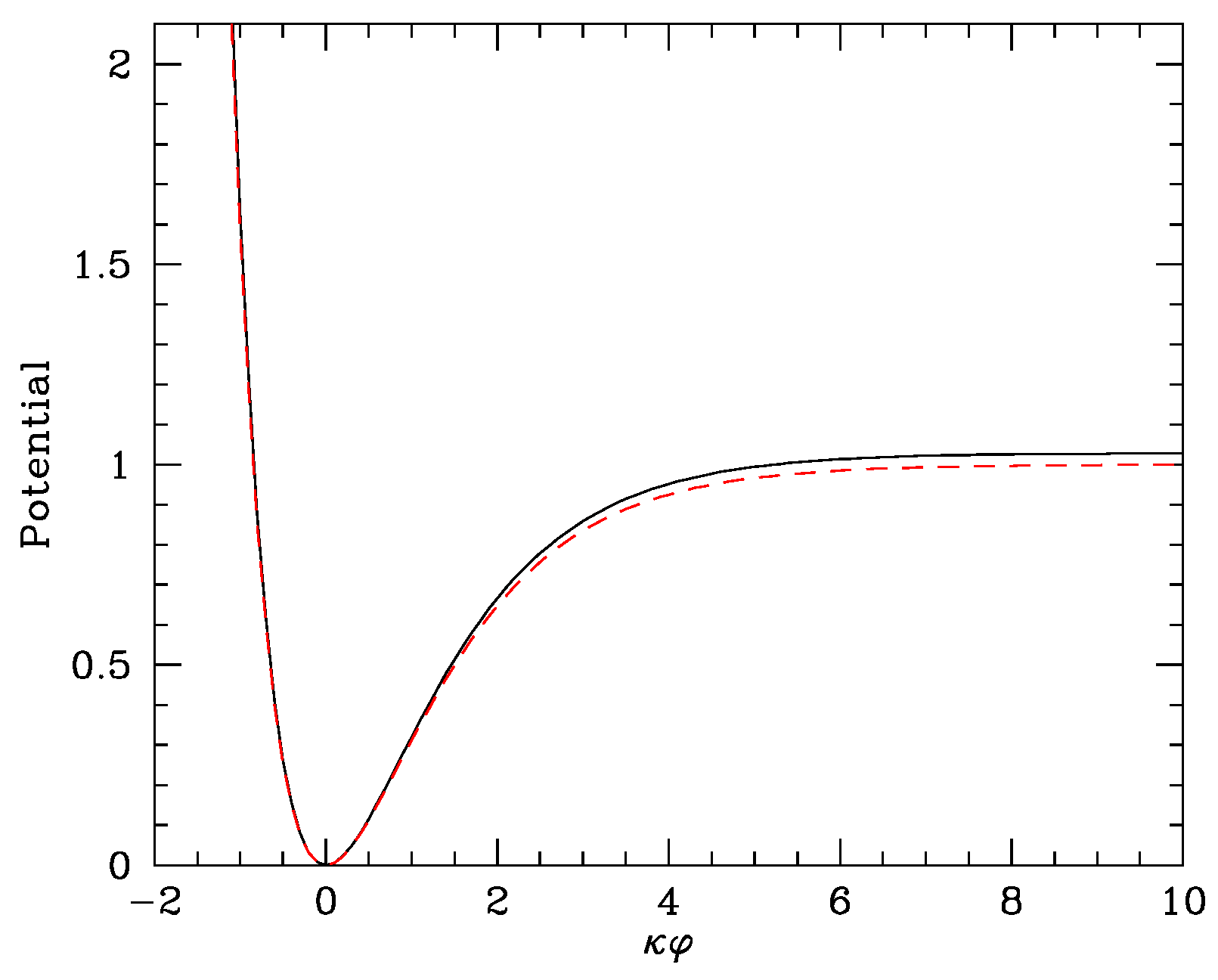
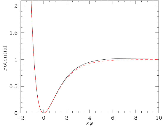
where the arrows have the meaning that the corresponding actions appear in the appropriate path integrals. The ensuing effective potential $V_{\mathrm{eff}}\left(\phi \right)$ is given by:

$$\begin{array}{c}\hfill V_{\mathrm{eff}}\left(\phi \right)=\frac{3{\mathcal{M}}^2{\left(1-e^{-\sqrt{\frac{2}{3}}\kappa \phi }\right)}^2}{4{\kappa }^2}.\end{array}$$

(8)

One can check that the mass of the scalaron, which can be seen as the new gravitational degree of freedom that the conformal transformation was able to elucidate from the Starobinsky action, is indeed given by the parameter $\mathcal{M}=\sqrt{8\pi /3\beta }$:

$${\left.\frac{d^2{V}_{\mathrm{eff}}\left(\phi \right)}{d{\phi }^2}\right|}_{\phi =0}={\mathcal{M}}^2.$$

(9)

Note that for $\phi =0$, one has $\tilde{\alpha }=0$, and the two conformally equivalent metrics coincide at this point. The effective potential for the scalar d.o.f. that conformally replaces the effect of the $R^2$ term is plotted in Figure 1.

We observe that $V\left(\phi \right)$ is sufficiently flat for $\kappa \phi =\phi /M_{Pl}\gg 1$ (i.e., for sufficiently large values of ϕ as compared to the reduced Planck scale) to produce phenomenologically-acceptable inflation. Obviously, the scalaron field ϕ is effectively playing the role of the inflaton in this context. The difference with the usual inflaton is that ϕ is not a new scalar d.o.f. imported from outside the gravitational action, but just an integral part of it, namely it is just a gravitational d.o.f. that describes in an effective (and very convenient) way the $\sim R^2$ term of (5). The Starobinsky model based on the action (5) indeed fits excellently with the Planck data on inflation [2,3,4] and, also, the corresponding data from the joint BICEP2-Planck analysis [6].

Quantum-gravity corrections in the original Starobinsky model (5) have been considered recently in [54] from the point of view of an exact re-normalisation-group analysis [55,56]. It was shown that the non-perturbative beta-functions for the ‘running’ of Newton’s ‘constant’ G and the dimensionless inverse $R^2$ coupling ${\kappa }^2{\beta }^{-1}\sim {\mathcal{M}}^2/M_{Pl}^2$ in (5) imply an asymptotically-safe ultraviolet (UV) fixed point for the former (that is, G($k\to \infty$) → constant, for some four-momentum cut-off scale k), in the spirit of Weinberg [57], and an attractive asymptotically-free (${\kappa }^2{\beta }^{-1}(k\to \infty )\to 0$) point for the latter. In this sense, the smallness of the (inverse) $R^2$ coupling, required for agreement with inflationary observables [2,3,4], is naturally ensured by the presence of the asymptotically-free UV fixed point.

The agreement of the model of [5] with the Planck data triggered an enormous interest in the current literature, and indeed, Starobinsky inflation has been revisited from various points of view, such as its connection with no-scale supergravity [58,59] and (super)conformal versions of supergravity and related areas [60,61,62,63,64,65,66,67]. In the latter works, however, the Starobinsky scalaron field is fundamental, arising from the appropriate scalar component of some chiral superfield that appears in the superpotentials of the model.

Although of great value, illuminating a strong connection between supergravity models and inflationary physics, and especially for explaining the low-scale of inflation compared to the Planck scale, these works contradict the original spirit of the Starobinsky model (5), where, as mentioned previously, the higher curvature corrections are viewed as arising from quantum fluctuations of matter fields in a curved spacetime background, such that inflation is driven by the pure gravity sector in the absence of fundamental scalars. On the other hand, the scenario of [9], in which a Starobinsky-type inflation arises in the massive gravitino phase of SUGRA models, after integrating out the massive degrees of freedom, is in the same spirit of Starobinsky and, even better, in the sense that the model does not have to assume the dominance of conformal matter during inflation.

We next proceed to summarize the construction of the one-loop effective action of the massless degrees of freedom after massive gravitino integration in this dynamically-broken SUGRA model with spontaneous breaking of global supersymmetry (SUSY) [7,8].

4. Starobinsky-Type Inflation in Dynamically-Broken SUGRA

Dynamical breaking of SUGRA, in the sense of the generation of a mass for the gravitino field ${\psi }_{\mu }$, whilst the gravitons remain massless, occurs in the model as a result of the four-gravitino interactions characterizing the SUGRA action, arising from the torsionful contributions of the spin connection, characteristic of local supersymmetric theories.

Our starting point is the $\mathcal{N}=1$$D=4$ (on-shell) action for ‘minimal’ Poincaré supergravity in the second order formalism [68,69]:

$$\begin{array}{c}{S}_{\mathrm{SG}}=\int d^{4}xe\left(\frac{1}{2{\kappa }^2}R\left(e\right)-{\overline{\psi }}_{\mu }{\gamma }^{\mu \nu \rho }{D}_{\nu }{\psi }_{\rho }+{\mathcal{L}}_{\mathrm{torsion}}\right),\hfill \\ {\kappa }^2=8\pi G,{\gamma }^{\mu \nu \rho }=\frac{1}{2}\left\{{\gamma }^{\mu },{\gamma }^{\nu \rho }\right\},{\gamma }^{\nu \rho }=\frac{1}{2}\left[{\gamma }^{\nu },{\gamma }^{\rho }\right],\hfill \end{array}$$

(10)

where $R\left(e\right)$ and $D_{\nu }{\psi }_{\rho }\equiv {\partial }_{\nu }{\psi }_{\rho }+\frac{1}{4}{\omega }_{\nu ab}\left(e\right){\gamma }^{ab}{\psi }_{\rho }$ are defined via the torsion-free connection; and given the gauge condition $\gamma ·\psi =0$,

$$\begin{array}{c}\hfill {\mathcal{L}}_{\mathrm{torsion}}=-\frac{{\kappa }^2}{8}\left({\overline{\psi }}^{\rho }{\gamma }^{\mu }{\psi }^{\nu }\right)\left({\overline{\psi }}_{\rho }{\gamma }_{\mu }{\psi }_{\nu }+2{\overline{\psi }}_{\rho }{\gamma }_{\nu }{\psi }_{\mu }\right),\end{array}$$

(11)

arising from the fermionic torsion parts of the spin connection. Extending the action off-shell requires the addition of auxiliary fields to balance the graviton and gravitino degrees of freedom. These fields however are non-propagating and may only contribute through the development of scalar vacuum expectation values, which would ultimately be re-summed into the cosmological constant.

Making further use of the above gauge condition together with the Fierz identities (as detailed in [7,8]), we may write:

$$\begin{array}{c}\hfill \frac{{\mathcal{L}}_{\mathrm{torsion}}}{{\kappa }^2}={\lambda }_{\mathrm{S}}{\left({\overline{\psi }}^{\rho }{\psi }_{\rho }\right)}^2+{\lambda }_{\mathrm{PS}}{\left({\overline{\psi }}^{\rho }{\gamma }^5{\psi }_{\rho }\right)}^2+{\lambda }_{\mathrm{PV}}{\left({\overline{\psi }}^{\rho }{\gamma }^5{\gamma }_{\mu }{\psi }_{\rho }\right)}^2,\end{array}$$

(12)

where the couplings ${\lambda }_{\mathrm{S}}$, ${\lambda }_{\mathrm{PS}}$ and ${\lambda }_{\mathrm{PV}}$ express the freedom we have to rewrite each quadrilinear in terms of the others via Fierz transformation. This freedom in turn leads to a known ambiguity in the context of (perturbative) mean field theory [70] and can only be resolved by a non-perturbative treatment.

Specifically, we wish to linearise these four-fermion interactions via suitable auxiliary fields, e.g.,

$$\begin{array}{c}\hfill \frac{1}{4}{\kappa }^2{\lambda }_S{\left({\overline{\psi }}^{\rho }{\psi }_{\rho }\right)}^2\sim \sigma \kappa \sqrt{{\lambda }_S}\left({\overline{\psi }}^{\rho }{\psi }_{\rho }\right)-{\sigma }^2,\end{array}$$

(13)

where the equivalence (at the level of the action) follows as a consequence of the subsequent Euler–Lagrange equation for the auxiliary scalar σ. Our task is then to look for a non-zero vacuum expectation value $\langle \sigma \rangle$, which would induce as an effective mass $m_{3/2}\sim \sigma \kappa \sqrt{{\lambda }_S}$ for the gravitino. This is however complicated by the fact that our coupling ${\lambda }_{\mathrm{S}}$ into this particular channel is, by virtue of Fierz transformations, ambiguous at a perturbative level, and as mentioned, in order to fix them, a fully non-perturbative treatment of SUGRA-like models would be required, which are not currently at hand. Nevertheless, there is another way out [7,8,10], whereby the Fierz ambiguities may be absorbed by dilaton-expectation-value shifts in an extension of $\mathcal{N}=1$ SUGRA, which incorporates local supersymmetry in the Jordan frame, enabled by an associated dilaton superfield [71,72]. The (logarithm of the) scalar component ϕ of the latter can be either a fundamental spacetime scalar mode of the gravitational multiplet, i.e., the trace of the graviton (as happens, for instance, in supergravity models that appear in the low-energy limit of string theories) or a composite scalar field constructed out of matter multiplets. In the latter case, these could include the standard model fields and their superpartners that characterise the next-to-minimal supersymmetric standard model [73], which can be consistently incorporated in such Jordan frame extensions of SUGRA.

Upon appropriate breaking of conformal symmetry, induced by specific dilaton potentials (which we do not discuss here), one may then assume that the dilaton field acquires a non-trivial vacuum expectation value $\langle \varphi \rangle \ne 0$, thus absorbing any ambiguities in the value of the appropriate coefficient ${\lambda }_S$ induced by Fierz (12). One consequence of this is then that in the broken conformal symmetry phase, the resulting supergravity sector, upon passing (via appropriate field redefinitions) to the Einstein frame, is described by an action of the form (10), but with the coupling of the gravitino four-fermion interaction terms being replaced by:

$${\tilde{\kappa }}^2\equiv {\lambda }_S{\kappa }^2=e^{-4\langle \varphi \rangle }{\kappa }^2,$$

(14)

while the Einstein term in the action carries the standard gravitational coupling $1/2{\kappa }^2$. For phenomenological reasons, associated with gravitino masses in the ball-park of GUT scales, one must have $\tilde{\kappa }\gg \kappa$. This is assumed to be guaranteed by appropriate microscopic dilaton potentials that break the (super)conformal symmetry of the Jordan-frame SUGRA appropriately.

To induce the super-Higgs effect [74], we couple to the action (10) the Goldstino associated to global supersymmetry breaking via the addition of:

$$\begin{array}{c}\hfill {\mathcal{L}}_{\lambda }=f^{2}det\left({\delta }_{\mu \nu }+\frac{i}{2f^2}\overline{\lambda }{\gamma }_{\mu }{\partial }_{\nu }\lambda \right){|}_{\gamma ·\psi =0}=f^2+\cdots ,\end{array}$$

(15)

where λ is the Goldstino, $\sqrt{f}$ expresses the scale of global supersymmetry breaking and ... represents higher order terms, which may be neglected in our weak-field expansion of the determinant. It is worth emphasising at this point the universality of (15); any model containing a Goldstino may be related to ${\mathcal{L}}_{\lambda }$ via a non-linear transformation [75], and thus, the generality of our approach is preserved.

Upon the aforementioned gauge choice for the gravitino field ${\gamma }^{\mu }{\psi }_{\mu }=0$ and an appropriate redefinition, one may eliminate any presence of the Goldstino field from the final effective action describing the dynamical breaking of local supersymmetry, except the cosmological constant term $f^2$ in (15), which serves as a reminder of the pertinent scale of supersymmetry breaking. The non-trivial energy scale this introduces, along with the disappearance (through field redefinitions) of the Goldstino field from the physical spectrum and the concomitant development of a gravitino mass, characterises the super-Higgs effect.

The linearisation of the four-gravitino terms (13), when combined with the $f^2$ term of the super-Higgs effect, implies a tree-level cosmological constant:

$$\begin{array}{c}\hfill \frac{{\Lambda }_0}{{\kappa }^2}\equiv {\sigma }^2-f^2,\end{array}$$

(16)

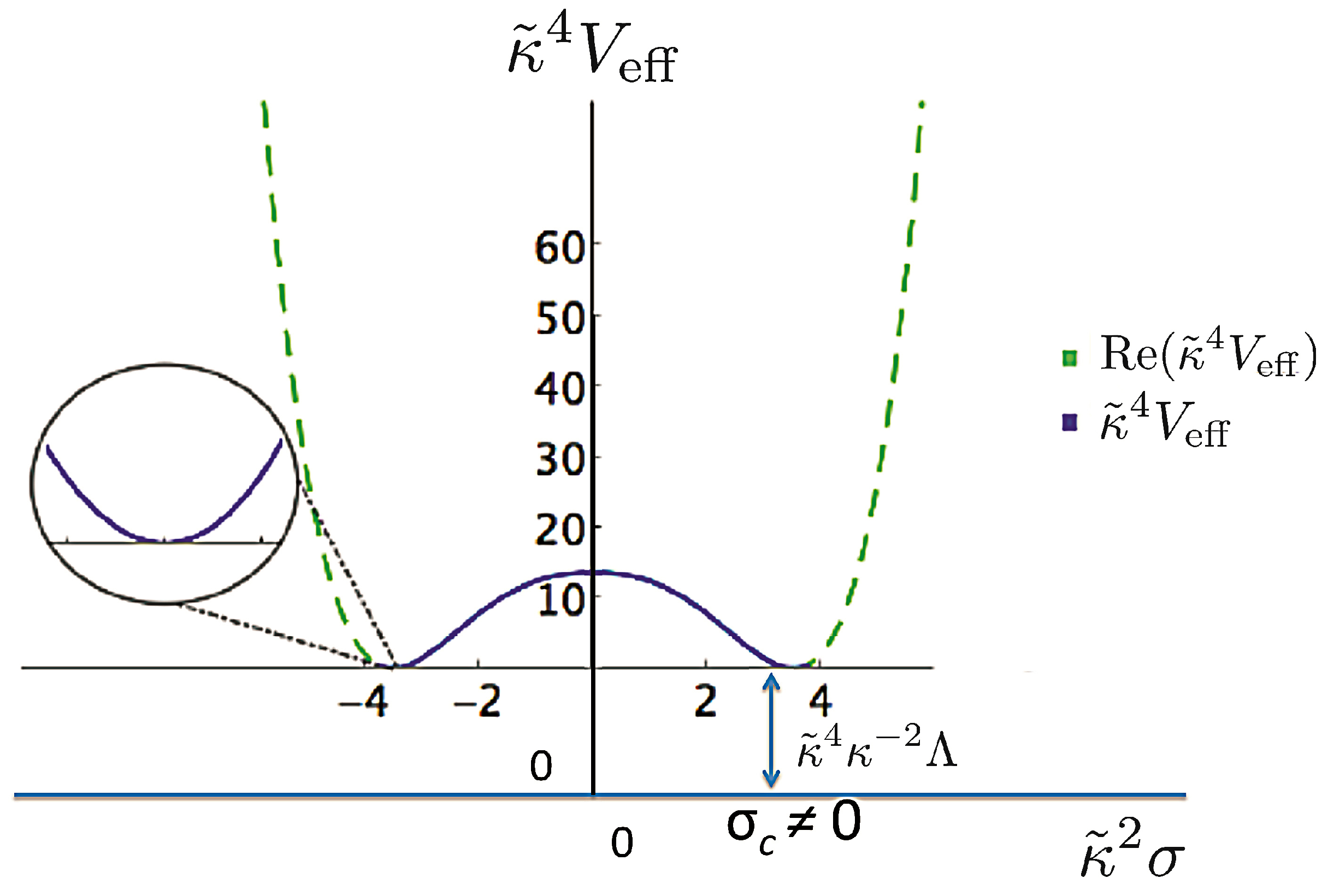
which must be negative due to the incompatibility of supergravity with de Sitter vacua (notice that in our conventions, both σ and f have dimension $+2$ in natural units).

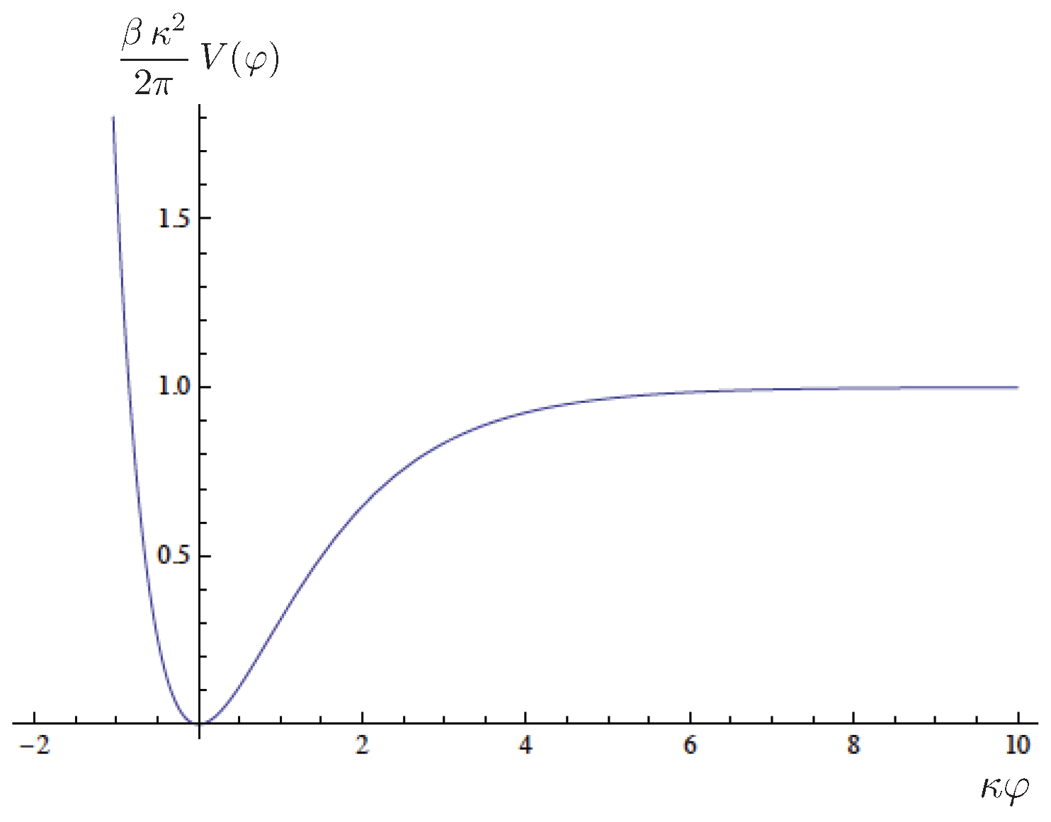
The one-loop effective potential for the scalar gravitino condensate field $\sigma \left(x\right)$ (with vacuum expectation value ${\sigma }_c\propto \langle {\overline{\psi }}_{\mu }{\psi }^{\mu }\rangle$) has a double-well shape as a function of $\sigma \left(x\right)$, which is symmetric about the origin (cf. Figure 2), as dictated by the fact that the sign of a fermion mass does not have physical significance. Dynamical generation of the gravitino mass occurs at the non-trivial minima corresponding to ${\sigma }_c\ne 0$. The potential of the ${\sigma }_c$ field is also flat near the origin, and this has been identified in [10] with a first inflationary phase.

In [7,8], the one-loop effective potential was derived by first formulating the theory on a curved de Sitter background [76,77], with cosmological constant (one-loop induced) $\Lambda >0$, not to be confused with the (negative) tree-level one ${\Lambda }_0$ (16), and then integrating out spin-two (graviton) and spin 3/2 (gravitino) quantum fluctuations in a given class of gauges (physical), before considering the flat limit $\Lambda \to 0$ in a self-consistent way. The detailed analysis in [7,8], performed in the physical gauge, has demonstrated that the dynamically-broken phase is then stable (in the sense of the effective action not being characterized by imaginary parts) provided the scale of the gravitino condensate is equal to or below the scale of spontaneous breaking of global SUSY:

$${\sigma }^2\le f^2,$$

(17)

which guarantees the aforementioned result on the necessity of the negative nature of the tree-level cosmological constant (16).

The former result demonstrates the importance of the existence of the global SUSY breaking scale for the stability of the phase where dynamical generation of gravitino masses occurs, which was not considered in the previous literature [78,79]. In super-conformal versions of SUGRA, e.g., those in [71,72,73], phenomenologically realistic scales for $f^2$ and gravitino mass of order of the GUT scale appear for appropriate values of the expectation value of the conformal factor. These imply inflationary scenarios in perfect agreement with the Planck data [2,3,4,10], on equal footing with the original Starobinsky model.

In [9], we considered an extension of the analysis of [7,8] to the case where the de Sitter parameter Λ is perturbatively small compared to $m_P^2$, but non-zero, so that truncation of the series to order ${\Lambda }^2$ suffices. This is in the spirit of the original Starobinsky model [5], with the role of matter fulfilled by the now-massive gravitino field. Specifically, we were interested in the behaviour of the effective potential near the non-trivial minimum, where $\sigma \simeq {\sigma }_c$ is a non-zero constant (cf. Figure 2). The one-loop effective potential, obtained by integrating out [76,77] gravitons and (massive) gravitino fields in the scalar channel (after appropriate Euclideanisation), may be expressed as a power series in Λ:

$$\Gamma \simeq S_{\mathrm{cl}}-\frac{24{\pi }^2}{{\Lambda }^2}({\alpha }_0^F+{\alpha }_0^B+\left({\alpha }_1^F+{\alpha }_1^B\right)\Lambda +\left({\alpha }_2^F+{\alpha }_2^B\right){\Lambda }^2+\cdots ),$$

(18)

where $S_{\mathrm{cl}}$ denotes the classical action with tree-level cosmological constant ${\Lambda }_0$ (to be contrasted with the one-loop cosmological constant Λ):

$$\begin{array}{c}\hfill -\frac{1}{2{\kappa }^2}\int d^{4}x\sqrt{g}\left(\widehat{R}-2{\Lambda }_0\right),{\Lambda }_0={\kappa }^2\left({\sigma }_c^2-f^2\right),\end{array}$$

(19)

with $\widehat{R}$ denoting the fixed $S^4$ background; we expand around ($\widehat{R}=4\Lambda$, and the four-dimensional Euclidean volume is $24{\pi }^2/{\Lambda }^2$); the α’s indicate the bosonic (graviton) and fermionic (gravitino) quantum corrections at each order in Λ. The reader should notice that, upon the restriction (17) guaranteeing the absence of imaginary parts in the one-loop effective action, the tree-level cosmological constant (16) ${\Lambda }_0<0$, while the one-loop one $\Lambda >0$, as appropriate for a de Sitter background. Thus, ${\Lambda }_0$ should not be confused with the current-epoch positive cosmological constant ${\tilde{\Lambda }}_0$, which we introduce later on, in Section 5.2, when we discuss the running vacuum model (RVM) (cf. (57)).

The leading order term in Λ is then the effective action found in [7,8] in the limit $\Lambda \to 0$,

$$\begin{array}{c}\hfill {\Gamma }_{\Lambda \to 0}\simeq -\frac{24{\pi }^2}{{\Lambda }^2}\left(-\frac{{\Lambda }_0}{{\kappa }^2}+{\alpha }_0^F+{\alpha }_0^B\right)\equiv \frac{24{\pi }^2}{{\Lambda }^2}\frac{{\Lambda }_1}{{\kappa }^2},\end{array}$$

(20)

with:

$$\begin{array}{c}\hfill {\Lambda }_1=-{\kappa }^2\left(-\frac{{\Lambda }_0}{{\kappa }^2}+{\alpha }_0^F+{\alpha }_0^B\right),\end{array}$$

(21)

where:

$$\begin{array}{c}{\alpha }_0^F={\tilde{\kappa }}^4{\sigma }_c^4\left(0.100ln\left(\frac{{\tilde{\kappa }}^2{\sigma }_c^2}{3{\mu }^2}\right)+0.126\right),\hfill \end{array}$$

(22)

and:

$$\begin{array}{c}\hfill {\alpha }_0^B={\kappa }^4{\left(f^2-{\sigma }_c^2\right)}^2\left(0.027-0.018ln\left(\frac{3{\kappa }^2\left(f^2-{\sigma }_c^2\right)}{2{\mu }^2}\right)\right),\end{array}$$

(23)

indicate the leading (as $\Lambda \to 0$) contributions to the effective potential from bosonic (graviton) and fermionic (gravitino) quantum fluctuations, respectively, to one-loop order. Above, μ is an RG scale, associated with a short-distance proper time cut-off [7,8], not to be confused with the RG scale of the RVM ${\mu }_c\left(t\right)$ (cf. Section 2), which is such that the flow from ultraviolet (UV) to infrared (IR) corresponds to the direction of increasing μ; ${\sigma }_c$ denotes the gravitino scalar condensate ${\sigma }_c\propto \tilde{\kappa }\langle {\overline{\psi }}_{\mu }{\psi }^{\mu }\rangle$ at the non-trivial minimum of the one-loop effective potential (cf. Figure 2); $\tilde{\kappa }$ is the conformally-rescaled gravitational constant in the Jordan-frame SUGRA model of [71,72], defined in (14), corresponding to a non-trivial v.e.v.of the conformal (‘dilaton’) factor, $\langle \varphi \rangle \ne 0$, assumed to be stabilized by means of an appropriate potential, leading to the breaking of the conformal symmetry. In the case of standard $\mathcal{N}=1$ SUGRA, $\langle \varphi \rangle =0$.

The remaining (higher order in Λ) one-loop quantum corrections then, proportional to Λ and ${\Lambda }^2$ may be identified respectively with Einstein–Hilbert R-type and Starobinsky $R^2$-type terms in an effective action of the form

$$\begin{array}{cc}\hfill \Gamma \simeq & -\frac{1}{2{\kappa }^2}\int d^{4}x\sqrt{g}\left[\left(\widehat{R}-2{\Lambda }_1\right)+{\alpha }_1\widehat{R}+{\alpha }_2{\widehat{R}}^2\right],\hfill \end{array}$$

(24)

where we have combined terms of order ${\Lambda }^2$ into curvature scalar square terms. The reader should recall at this stage that the sign of g in $\sqrt{g}$ and the overall minus sign in front of the right-hand-side of (24) is due to the Euclidean-signature formulation of the path integral and disappears upon analytic continuation back to the Minkowski spacetime at the end of the computations, which is necessary in order to make contact with phenomenology/cosmology (see, e.g., (5)). This should be understood in what follows, and especially in the context of linking the SUGRA model with the RVM in Section 5.

For general backgrounds, such terms would correspond to invariants of the form ${\widehat{R}}_{\mu \nu \rho \sigma }{\widehat{R}}^{\mu \nu \rho \sigma }$, ${\widehat{R}}_{\mu \nu }{\widehat{R}}^{\mu \nu }$ and ${\widehat{R}}^2$, which for a de Sitter background all combine to yield ${\widehat{R}}^2$ terms. In the pure SUGRA case, with no dilaton frame functions, the fact that the Gauss–Bonnet combination $R_{\mu \nu \rho \sigma }{R}^{\mu \nu \rho \sigma }-4R_{\mu \nu }{R}^{\mu \nu }+R^2$ is a total derivative in four spacetime dimension implies that one can consider only the Ricci-scalar and Ricci-tensor squared terms as independent. This is not the case though in the conformal SUGRA case [71,72].

The coefficients ${\alpha }_1$ and ${\alpha }_2$ in (24) absorb the non-polynomial (logarithmic) in Λ contributions, so that we may then identify (24) with (18) via:

$$\begin{array}{c}\hfill {\alpha }_1=\frac{{\kappa }^2}{2}\left({\alpha }_1^F+{\alpha }_1^B\right),{\alpha }_2=\frac{{\kappa }^2}{8}\left({\alpha }_2^F+{\alpha }_2^B\right),\end{array}$$

(25)

where we note that ${\alpha }_1$ is dimensionless, whereas ${\alpha }_2$ has the dimension of inverse mass squared. The coefficients ${\alpha }_i^{F,B}$, $i=1,2$ in Equation (25) can be computed using the results of [7,8], derived via an asymptotic expansion:

$$\begin{array}{ccc}\hfill {\alpha }_1^F& =& 0.067{\tilde{\kappa }}^2{\sigma }_c^2-0.021{\tilde{\kappa }}^2{\sigma }_c^2\ln \left(\frac{\Lambda }{{\mu }^2}\right)+0.073{\tilde{\kappa }}^2{\sigma }_c^2\ln \left(\frac{{\tilde{\kappa }}^2{\sigma }_c^2}{{\mu }^2}\right),\hfill \\ \hfill {\alpha }_2^F& =& 0.029+0.014\ln \left(\frac{{\tilde{\kappa }}^2{\sigma }_c^2}{{\mu }^2}\right)--0.029\ln \left(\frac{\Lambda }{{\mu }^2}\right),\hfill \end{array}$$

(26)

and:

$$\begin{array}{ccc}\hfill {\alpha }_1^B& =& -0.083{\Lambda }_0+0.018{\Lambda }_0\ln \left(\frac{\Lambda }{3{\mu }^2}\right)+0.049{\Lambda }_0\ln \left(-\frac{3{\Lambda }_0}{{\mu }^2}\right),\hfill \\ \hfill {\alpha }_2^B& =& 0.020+0.021\ln \left(\frac{\Lambda }{3{\mu }^2}\right)-0.014\ln \left(-\frac{6{\Lambda }_0}{{\mu }^2}\right).\hfill \end{array}$$

(27)

To identify the conditions for phenomenologically-acceptable Starobinsky inflation around the non-trivial minima of the broken SUGRA phase of our model, we impose first the cancellation of the “classical” Einstein–Hilbert space term $\widehat{R}$ by the “cosmological constant” term ${\Lambda }_1$, i.e., that:

$$\widehat{R}=4\Lambda =2{\Lambda }_1\equiv -2{\kappa }^2\left(-\frac{{\Lambda }_0}{{\kappa }^2}+{\alpha }_0^F+{\alpha }_0^B\right)>0.$$

(28)

This condition should be understood as a necessary one characterizing our background in order to produce phenomenologically-acceptable Starobinsky inflation in the broken SUGRA phase following the first inflationary stage, as discussed in [10]. This may naturally be understood as a generalization of the relation $\widehat{R}=2{\Lambda }_1=0$, imposed in [7,8] as a self-consistency condition for the dynamical generation of a gravitino mass in the flat (zero Λ) limit.

From Equation (28), it follows that the (positive) cosmological constant $\Lambda >0$ satisfies the four-dimensional Einstein equations in the non-trivial minimum and, in fact, coincides with the value of the one-loop effective potential of the gravitino condensate at this minimum. As we discussed in [7,8], this non-vanishing positive value of the effective potential is consistent with the generic features of dynamical breaking of supersymmetry [80]. In terms of the Starobinsky inflationary potential (8), the value $\Lambda >0$ corresponds to the approximately constant value of this potential in the high ϕ-field regime ($\kappa \phi \gg 1$) of Figure 1, in the flat region where Starobinsky-type inflation takes place. Thus, we may set:

$$\Lambda \sim 3H_I^2,$$

(29)

where $H_I$ is the (approximately) constant Hubble scale during inflation, which is constrained by the current data to satisfy (2) or (3). In the SUGRA context under discussion, $H_I$ is linked to the scale of global SUSY breaking through $H_I\simeq f/M_{Pl}$.

The effective Newton’s constant in (24), after the imposition of (28), is then defined as:

$${\kappa }_{\mathrm{eff}}^2=\frac{{\kappa }^2}{{\alpha }_1},$$

(30)

and from this, we can express the effective Starobinsky parameter (5) in terms of ${\kappa }_{\mathrm{eff}}$ as:

$${\beta }_{\mathrm{eff}}\equiv \frac{{\alpha }_2}{{\alpha }_1}.$$

(31)

This condition thus makes a direct link between the action (18) with a Starobinsky type action (5). Comparing to (5), we can determine the effective scalaron mass in this case:

$$\mathcal{M}=\sqrt{\frac{8\pi }{3}\frac{{\alpha }_1}{{\alpha }_2}},$$

(32)

As we know, this mass parameter also sets the order of magnitude of the inflationary scale in the Starobinsky model.

We may then determine the coefficients ${\alpha }_1$ and ${\alpha }_2$ in order to evaluate the scale $1/\sqrt{\beta }\sim \mathcal{M}$ of the effective Starobinsky potential given in Figure 1 in this case and, thus, the scale of the second inflationary phase.

In [9], we searched numerically for points in the parameter space, such that:

• The effective equations

  $$\begin{array}{c}\hfill \frac{\partial \Gamma }{\partial \Lambda }=0,\frac{\partial \Gamma }{\partial \sigma }{|}_{\sigma ={\sigma }_c}=0,\end{array}$$

  (33)

  are satisfied, together with the condition (28):
• The cosmological constant Λ is small and positive, satisfying (29), and for phenomenological reasons, it should be of order:

  $$0<\Lambda \sim {10}^{-10}{M}_{\mathrm{Pl}}^2,$$

  (34)

  to ensure the validity of our expansion in Λ, consistent with the phenomenology of Planck-satellite data [2,3,4].
• The scalaron mass should also be of order $\mathcal{M}\sim {10}^{-5}{M}_{\mathrm{Pl}}$, hence allowing us to achieve phenomenologically-acceptable Starobinsky inflation in the massive gravitino phase, consistent with the Planck-satellite data [2,3,4].

For $\tilde{\kappa }=\kappa$ (i.e., for non-conformal supergravity), we were unable to find any solutions satisfying these constraints. This, of course, may not be surprising, given the previously demonstrated non-phenomenological suitability of this simple model [7,8]. If we consider $\tilde{\kappa }\gg \kappa$, however, we find that we are able to satisfy the above constraints for a range of values. A comment concerning SUGRA models in the Jordan frame with such large values for their frame functions is in order here. In our approach, the dilaton $2\varphi$ could be a genuine (dimensionless) dilation scalar field arising in the gravitational multiplet of string theory, whose low-energy limit may be identified with some form of SUGRA action. In our normalization, the string coupling would be $g_s\equiv e^{\varphi }={\left(\tilde{\kappa }/\kappa \right)}^{-1/2}$. In such a case, a value of $\tilde{\kappa }=e^{-2\langle \varphi \rangle }\kappa =\mathcal{O}\left({10}^{3-4}\right)\kappa$ would imply a large negative v.e.v. of the (four-dimensional) dilaton field of order $\langle \varphi \rangle =-\mathcal{O}\left(5\right)<0$ and, thus, a weak string coupling squared $g_s=\mathcal{O}\left({10}^{-2}\right)$, which may not be far from the values attained in realistic phenomenological string models. On the other hand, in the Jordan-frame SUGRA models of [71,72], the frame function reads $\Phi \equiv e^{-2\varphi }=1-\frac{1}{3}\left(S\overline{S}+{\sum }_{u,d}{H}_i{H}_i^{†}\right)-\frac{1}{2}\chi \left(-H_u^0{H}_d^0+H_u^{+}{H}_d^{-}+\mathrm{h}.\mathrm{c}.\right)$, in the notation of [73] for the various matter super fields of the next-to-minimal supersymmetric standard model that can be embedded in such supergravities. The quantity χ is a constant parameter. At energy scales much lower than GUT, it is expected that the various fields take on sub-Planckian values, in which case the frame function is almost one and, hence, $\tilde{\kappa }\simeq \kappa$ for such models today. To ensure $\tilde{\kappa }\gg \kappa$ and, thus, large values of the frame function, $\Phi \gg 1$, as required in our analysis, one needs to invoke trans-Planckian values for some of the fields, $H_{u,d}^0$, and large values of χ, which may indeed characterize the inflationary phase of such theories. A similar situation occurs for the values of the Higgs field (playing the role of the inflaton) in the non-supersymmetric Higgs inflation models [81,82]).

In general, typical values obtained in phenomenological-realistic conformal SUGRA models satisfy $\tilde{\kappa }\gg \kappa$ (e.g., of order $\tilde{\kappa }/\kappa =\mathcal{O}({10}^3-{10}^4))$, under the constraints (29) and (34), in such a way that:

$$\Lambda \sim 3H_I^2\sim m_{3/2}^2\sim {\tilde{\kappa }}^2{\sigma }_c^2\sim {\kappa }^2{f}^2\ll {\mu }^2=8\pi /{\kappa }^2,{\sigma }_c^2\ll f^2.$$

(35)

Since the scale of SUSY breaking must be in the ballpark of the typical GUT scale associated with the inflation, namely $\sqrt{f}\sim {10}^{16}$ GeV$\sim {10}^{-2}{M}_{Pl}$, from the above, we have $\Lambda \sim {\kappa }^2{f}^2=f^2/M_{Pl}^2\sim {10}^{27}$ GeV${}^2$. As a result, the scale of the gravitino is some two to three orders of magnitude below the GUT scale, that is to say, $m_{3/2}\sim \sqrt{\Lambda }\gtrsim {10}^{13}$ GeV$\sim {10}^{-5}{M}_{Pl}$. These values are compatible with both the combined Planck and Bicep2 bound (3) and the typical mass of the gravitino in this framework [9].

Exit from the inflationary phase is, of course, a complicated issue, which we shall not discuss here at the level of the SUGRA model itself, aside from the observation that it can be achieved by coherent oscillations of the gravitino condensate field around its minima and subsequent decays to radiation and matter fields (thus requiring detailed knowledge of the matter content of the SUGRA models in order to arrive at quantitative predictions for the exit phase) or tunnelling processes à la Vilenkin [51]. However, in the next section, we will show that the SUGRA model can be represented by an effective running vacuum model along the lines indicated in Section 2, and from this point of view, the exiting from the inflationary phase into the standard radiation phase can be guaranteed on very general grounds.

Before doing so, though, we should make some important remarks concerning the presence of logarithms of the de Sitter scale Λ in the coefficients ${\alpha }_i$ of the curvature terms of the effective action (24). When one computes the effective action in a fixed de Sitter background, it is tempting to identify a Λ term with the Ricci scalar, which eventually will be allowed to depend on time. Thus, naively, the presence of logarithms would imply non-polynomial terms of the form $R\ln R$, which would be problematic for any RVM interpretation of the exit from the inflationary phase, as it would contradict the spirit of the approach where only integer powers of the curvature terms would be allowed in the respective flow equations [13,14,15,17,18,19,20,21,22]. Fortunately, this is not the case. To understand this, we first remark that any effective action obtained by integrating out massive degrees of freedom, such as gravitino fields, which we restrict ourselves here, must consist for reasons of covariance and consistency of the weak gravitational fluctuations about the de Sitter background only of polynomial structures of the curvature tensors, for instance to fourth order in derivatives terms involving the squares of the Ricci scalar and Ricci tensors and covariant derivatives thereof. Any $R\ln R$ term would be incompatible with the weak gravity perturbative expansion about a background, say of constant non-zero curvature.

Thus, the coefficients ${\alpha }_1$ and ${\alpha }_2$ in the action (24) are kept fixed, not undergoing temporal evolution, which is guaranteed by the fixing of the two free scales in the problem μ (35) and Λ (29). Notice that the scale μ should not be confused with the subsequent RG scale ${\mu }_c\left(t\right)$ that describes the cosmological evolution of the RVM vacuum (cf. Section 2). Indeed, the scale μ first of all is a high energy cut-off. As already mentioned, it plays the role of a proper-time cut-off scale [7,8], appearing in the integral representations of some ζ-functions that are part of the determinants arising in the path integral of the SUGRA action arising from integrating out massive spin 3/2 (gravitino) and spin two (graviton) fluctuations about the de Sitter background. The scale μ is therefore, in contrast to ${\mu }_c\left(t\right)$, an inverse re-normalization group scale. Its value has to be fixed so as to guarantee SUGRA breaking and to generate a fixed gravitino mass, which should not depend on time. This implies that the spontaneous breaking of SUGRA and the inflationary phase are characterised by such fixed scales, which implies the time independence of Λ (or, equivalently, the Hubble parameter) during inflation, the gravitino mass, related to the gravitino condensate vacuum expectation value ${\sigma }_c$ and, thus, the coefficients ${\alpha }_1$ and ${\alpha }_2$. On the other hand, integer positive powers of Λ appearing in the effective action may be replaced by higher order tensorial structures involving the square of the curvature tensors, which are allowed to vary with the cosmic time during the RVM phase after exiting from inflation. Notice that microscopically, the exit phase is characterised by an unknown sort of phase transition, either through decays of the gravitino condensates to matter parts and reheating of the inflated Universe, or tunnelling, as mentioned previously, and thus, using different RG running to relate various eras of the Universe after inflation is to be expected.

5. “Decay” of Effective Vacuum Energy: Running Vacuum Model

The main aim of this section is to demonstrate that there exists a family of time-dependent effective vacuum energy decaying models of running type, i.e., the class of the running vacuum models (RVMs) introduced in Section 2, which characterize the evolution of the Universe from the exit of the Starobinsky inflationary phase till the present era. In fact, the RVMs are able to interpolate on very general grounds the primeval de Sitter epoch with the late time de Sitter era, i.e., the dark energy one, where a much smaller cosmological constant essentially dominates. We shall follow the approach of the RVM outlined in Section 2, in which the vacuum energy density ${\rho }_{\Lambda }\left(H\right)$ varies with time through its dependence on $H=H\left(t\right)$. The Hubble parameter, having the dimension of energy in natural units, acts as the natural running scale via the RG equation Equation (4). As mentioned in Section 2, only the even powers of H can be involved in that equation, owing to the general covariance of the effective action. This is an important point to make possible a general QFT description of this RG approach and is essential for the connection with the SUGRA model under discussion.

It is evident that the expansion (4) quickly converges at low energies, where H is rather small; certainly much smaller than any particle mass. No other $H^{2n}$-term beyond $H^2$ (not even $H^4$) can contribute significantly to the r.h.s. of Equation (4) at any stage of the cosmological history below the GUT scale $M_X\sim {10}^{16}$ GeV, where presumably inflation occurs.

On the other hand, if we want to deal with the physics of inflation and in general the very early states of the cosmic evolution, we have to keep at least the term $H^4$, which in fact is the dominant term in the series (4) during the high energy regime. In contrast, the terms $H^6/M_i^2$ and above are less and less important, because these higher and higher powers of H are suppressed by the inverse powers of the heavy fermion and boson masses in the GUT, as required by the Appelquist–Carazzone decoupling theorem. Therefore, the dominant part of the series (4) is expected to be naturally truncated at the $H^4$ term. Higher order terms should contain the bulk of the high energy contributions within quantum field theory in curved spacetime, namely within a semi-classical description of gravity near, but (possibly a few orders) below the Planck scale. Models of inflation based on higher order terms inspired by the RG framework have existed for a long time in the literature (see [14,15]), as well as the unified inflation-dark energy framework of [13]. For a more phenomenological treatment unrelated to the RG, see [83,84,85,86].

5.1. A Distinct Class of Running Vacuum Models

Based on the above arguments, it is natural to consider the case in which the highest power of the Hubble rate in the RG Equation (4) is $H^4$. Integrating the RG equation provides the simplest realization of RVM that can describe inflation and the various stages of the FLRW regime:

$${\rho }_{\Lambda }\left(H\right)=\frac{\Lambda \left(H\right)}{{\kappa }^2}=\frac{3}{{\kappa }^2}\left(c_0+\nu H^2+\alpha \frac{H^4}{H_I^2}\right).$$

(36)

Here, $c_0$ is an integration constant (with dimension $+2$ in natural units, i.e., energy squared), which can be fixed from the low energy data of the current Universe [29,32]. On the other hand, the dimensionless coefficients are given as follows:

$$\nu =\frac{1}{48{\pi }^2}\sum _{i=F,B}{a}_i\frac{M_i^2}{M_{\mathrm{Pl}}^2},$$

(37)

and:

$$\alpha =\frac{1}{96{\pi }^2}\frac{H_I^2}{M_{\mathrm{Pl}}^2}\sum _{i=F,B}{b}_i.$$

(38)

At this point, we would like to make some comments that will hopefully make the reader appreciate the physical interpretation of the running vacuum scenario. The coefficient ν behaves as the reduced (dimensionless) beta-function for the RG running of ${\rho }_{\Lambda }$ at low energies, whereas α plays a similar role at high energies. Notice that the index i depends on whether bosons (B) or fermions (F) dominate in the loop contributions. Of course, since the coefficients $(\nu ,\alpha )$ play the role of one-loop beta-functions (at the respective low and high energy scales), they are expected to be naturally small because $M_i^2\ll M_{\mathrm{Pl}}^2$ for all of the particles, even for the heavy fields of a typical GUT. Indeed, an estimate of ν within a generic GUT is found in the range $\left|\nu \right|={10}^{-6}-{10}^{-3}$ [13]. The dimensionless coefficient α is also small, $\left|\alpha \right|\ll 1$, because the inflationary scale $H_I$ is certainly below the Planck scale; see Equation (3). From the observational viewpoint, utilizing a joint likelihood analysis of the recent supernovae Type Ia data, the CMB shift parameter and the baryonic acoustic oscillations, it has been found $\left|\nu \right|=\mathcal{O}\left({10}^{-3}\right)$ [29,30,32,33], which is nicely in accordance with the aforementioned theoretical expectations, as well as it ensures a mild dynamical behaviour of the vacuum energy at low energies. As we have already stated in Section 2, the quantum-gravity corrections in the Starobinsky model have been found in the context of the RG analysis [54,55,56] through the appropriate beta-functions. The fact that the nature of the main coefficients of both theories (running vacuum and Starobinsky) are based on the RG approach is a hint that perhaps there is a possible connection between the two models.

Indeed, as we will confirm below, this is the case. In particular, let us start with the effective action (24), with the coefficients (25)–(27) and the constraints (28) and (35). As we have seen, this action was obtained after integrating out both quantum-gravity (metric) fluctuations and massive gravitino fields. The action admits dynamical solutions of de Sitter vacua with a small cosmological constant Λ of order less than the GUT scale at early epochs of the Universe. At the non-trivial minimum, the effective potential takes on a value of order Λ (cf. Figure 2). Around the minimum, we should replace Λ by an effective Hubble parameter during inflation, $H_I$; Equation (29).

At the end of the day, the effective (dynamical) vacuum energy density, ${\rho }_{\Lambda }\left(H\right)$, during the inflationary phase of our SUGRA model can be extracted from the SUGRA effective action Γ (24), upon applying the constraint (28) and analytically continuing the results back to Minkowski spacetime signature. In particular, the effective potential is defined as $V_{\mathrm{eff}}\equiv -\Gamma \to \int d^{4}x\sqrt{-g}{\rho }_{\Lambda }\left(H\right)$. Doing so, we observe that the so-obtained ${\rho }_{\Lambda }\left(H\right)$, remarkably, adopts precisely the generic RVM structure (36) around that phase, in which the Ricci scalar (see Equation (50) below) boils down to $R\simeq 12H^2$ since H remains (approximately) constant in this phase.

Some important remarks are in order here. The imposition of the constraint (28) during the Starobinsky inflationary phase implies, as already mentioned, that the correct phenomenology is attained as a result of the effective gravitational coupling (30) that characterises that phase. Therefore, if the constraint was an exact result, the effective vacuum energy density of the SUGRA model would then correspond to the ${\widehat{R}}^2\to 144H^4$ terms in (24) with (30) playing the role of the effective gravitational constant,

$${\rho }_{\Lambda }^{\mathrm{SUGRA}}{\left(H\right)}_{\mathrm{constraint}}^{\mathrm{exact}}=\frac{72}{{\kappa }_{\mathrm{eff}}^2}\frac{{\alpha }_2}{{\alpha }_1}{H}^4=\frac{18}{{\kappa }_{\mathrm{eff}}^2}\frac{{\alpha }_2^F+{\alpha }_2^B}{{\alpha }_1^F+{\alpha }_1^B}{H}^4,$$

(39)

where we used (25)–(27). The form (39) constitutes an admissible class of RVM (cf. Equation (36)). Notice that in Equation (39), there is no ν term. This is important, in the sense that in such a model, as a result of the effective gravitational constant (30) entering the game, which in this scenario [9] is viewed as the ‘physical’ reduced Planck mass of order ${10}^{18}$ GeV, the gravitino mass and global SUSY breaking scales, (35), when expressed in terms of ${\kappa }_{\mathrm{eff}}$ are of order one; that is, one encounters a Planck-scale gravitino. Despite this, the vanishing of ν makes the re-normalization-group Equation (39) a consistent one within the perturbative class of (36).

However, the above construction leads to the absence of a present-era (small, positive) cosmological constant $c_0$. This arises from the fact that we imposed the constraint (28) exactly. It may well be that such a condition leaves (non-perturbatively, when all of the higher than one-loop contributions are taken into account) a very small (constant in cosmic time) contribution $c_0>0$, which is preserved until the present day. Unfortunately, our one-loop construction does not allow us to explain the magnitude and the sign of this constant term, but this is equivalent to offering a solution to the cosmological constant problem, which of course our approximate one-loop analysis cannot provide. While we do not have a quantitative calculation at this point, the above argument provides at least an interesting qualitative explanation, to wit: the origin of the current cosmological term ${\rho }_{\Lambda }^0$ in the model might well be attributed to quantum (non-perturbative) effects in the SUGRA effective action, which prevent the complete cancellation (28) from being realised. The constant residue $c_0$ is then transferred throughout the cosmic history and pops up in our days in the form of the tiny vacuum energy ${\rho }_{\Lambda }^0=(3/{\kappa }^2)(c_0+\nu H_0^2)\simeq 3c_0/{\kappa }^2$.

Under this assumption, then, the initial gravitational coupling κ and, thus, the Einstein term $\frac{1}{2{\kappa }^2}\int d^{4}x\sqrt{-g}\widehat{R}$ would enter the game during the exit phase from inflation. The reader should bear in mind that, since during the inflationary phase, the scalar degree of freedom of the Starobinsky action is slowly rolling, if there is inflation in the conformally-rescaled metric (6), there is also inflation in the initial metric. The Starobinsky inflation arguments are also not affected if a small contribution to the cosmological constant, of order of the present-era one, enters the effective action (7), as this is negligible compared to the Hubble scale of inflation. In such a case, in the exit phase, the effective vacuum energy of the SUGRA model at the inflationary phase should correspond to both ${\alpha }_1$ and ${\alpha }_2$ terms of (24), with the constraint (28) failing by a tiny amount ${\tilde{c}}_0>0$ corresponding to the present-era cosmological constant.

$${\rho }_{\Lambda }^{\mathrm{SUGRA}}\left(H\right)=\frac{1}{{\kappa }^2}\left({\tilde{c}}_0+6{\alpha }_1{H}^2+72{\alpha }_2{H}^4\right),$$

(40)

where the explicit form of the coefficients ${\alpha }_i$, $i=1,2$, given by Equations (25)–(27), in which the scales μ and Λ are fixed through (29) and (35), respectively. As mentioned already, fixing of the scale μ and Λ, implies fixed values for the gravitino mass.

It is worth stressing that the aforementioned ambiguity concerning the failure of the exact constraint (28) can be avoided altogether by observing that the corresponding ${\rho }_{\Lambda }\left(H\right)$ ultimately derives from the RG Equation (4) discussed in Section 2. It is therefore more appropriate, and elegant, if one performs the matching between the running vacuum energies ${\rho }_{\Lambda }\left(H\right)$ in the SUGRA model and RVM by equating the corresponding “RG beta” functions, $\frac{d{\rho }_{\Lambda }}{d\ln H^2}$:

$$\begin{array}{ccc}\hfill \frac{d{\rho }_{\Lambda }}{d\ln H^2}& =& 6{\kappa }^{-2}{\alpha }_1{H}^2+144{\kappa }^{-2}{\alpha }_2{H}^4\hfill \\ & \simeq & 3({\alpha }_1^F+{\alpha }_1^B)H^2+18({\alpha }_2^F+{\alpha }_2^B)H^4.\hfill \end{array}$$

(41)

It is remarkable that the effective dynamical vacuum energy density ${\rho }_{\Lambda }\left(H\right)$ associated with the SUGRA model under consideration turns out to follow the general RG of the RVM (see Equation (4)) in which the coefficients of the $H^2$ and $H^4$ terms can be computed precisely from the underlying SUGRA framework.

From Equation (41), it follows that ${\rho }_{\Lambda }={\rho }_{\Lambda }\left(H\right)$ evolves (“runs”) with the (time-evolving) value of H. Such evolution will be studied in more detail in the next section, but is relatively small in the beginning, namely the varying H is only slightly below the initial value given in Equation (29). As a result, the Universe can start with an initial inflationary phase, which is dominated by the $\sim H^4$ term of (41). However, well after the inflationary period, the $\sim H^2$-term takes over and remains in force until the present time, thereby providing a mild evolution of the current cosmological “constant”.

Eventually, one has to add to the effective action loop contributions from other matter fields, including particle multiplicities, but at the moment, we take a mass of order of the gravitino mass and shall comment on the possible additional effects below. The value of $m_{3/2}$ is of order of the GUT scale, since it is proportional to the gravitino condensate through ${\sigma }_c\sim {\tilde{\kappa }}^{-1}{m}_{3/2}$, the latter being bounded from above by the GUT scale: $\sqrt{{\sigma }_c}\le \sqrt{f}\sim {10}^{-2}{M}_{\mathrm{Pl}}$ (see Equation (17)). We must also keep in mind that for phenomenologically-acceptable solutions of the broken SUGRA model, the ratio $r\equiv \tilde{\kappa }/\kappa$ is forced to stay in the range $r=\mathcal{O}({10}^3-{10}^4)$.

From the generic values (35) we adopt here, we find:

$$\begin{array}{c}\hfill \frac{d{\rho }_{\Lambda }}{d\ln H^2}\sim 1.59{\tilde{\kappa }}^2{\sigma }_c^2{H}^2+25.76H^4.\end{array}$$

(42)

The integrated form of Equation(42) yields of course the effective vacuum energy density at the scale H, ${\rho }_{\Lambda }\left(H\right)$, Equation (40), within the current SUGRA scenario. We thus have:

$${\rho }_{\Lambda }\left(H\right)\simeq {\tilde{c}}_0+1.59{\tilde{\kappa }}^2{\sigma }_c^2{H}^2+12.88H^4,$$

(43)

where ${\tilde{c}}_0$ is the integration constant, which will play the role of the current-era cosmological constant, as already mentioned. The result naturally adopts the generic form of the canonical RVM, Equation (36) with $c_0={\kappa }^2{\tilde{c}}_0/3$ and the effective values for the coefficients ν and α given by:

$$\begin{array}{ccc}\hfill {\nu }_{\mathrm{eff}}& \simeq & 0.53{\kappa }^2{\tilde{\kappa }}^2{\sigma }_c^2\simeq \mathcal{O}\left(\frac{m_{3/2}^2}{M_{\mathrm{Pl}}^2}\right),\hfill \end{array}$$

(44)

$$\begin{array}{ccc}\hfill {\alpha }_{\mathrm{eff}}& \simeq & 4.30H_I^2{\kappa }^2\simeq \mathcal{O}\left(\frac{H_I^2}{M_{\mathrm{Pl}}^2}\right).\hfill \end{array}$$

(45)

Thus, we observe that, within the context of the pure SUGRA model, where only the gravitino plays the role of “matter”, both coefficients are small, of typical order ${10}^{-9}$, in accordance with their interpretation as β-function coefficients of the running vacuum energy density. Let us also note that the above estimate for ${\nu }_{\mathrm{eff}}$ nicely fits with the formal expression obtained in the different context of anomaly-induced inflation, where it also takes the structure (37), namely a quantity proportional to the (squared) ratio of a heavy particle scale (in general, a collection of them) to the Planck mass; see [13] for details. In the full SUGRA case, after its coupling to ordinary matter and radiation fields, other SUSY heavy fermions with masses near the SUSY breaking scale should also contribute to ${\nu }_{\mathrm{eff}}$ and α, and this should enhance the value of this coefficient very significantly, thus bringing the obtained result even closer to the situation studied in [13]. Overall, such considerations in phenomenologically-realistic SUGRA situations could bring these parameters to a range $\sim {10}^{-4}$ accessible to current observations [29,30].

We next remark that, in the general case where the parameters of the SUGRA model are varied from the generic values considered in (35), but within the allowed range, the values of ${\nu }_{\mathrm{eff}}$ and ${\alpha }_{\mathrm{eff}}$ can also undergo some variation, and the sign of ${\nu }_{\mathrm{eff}}$ could change. However, we stress that the sign of ${\alpha }_{\mathrm{eff}}$ remains always positive, which is essential for a correct description of inflation. This can be seen explicitly by comparing the various logarithms involved in the structure of the coefficient ${\alpha }_2$ of the $H^4$-term in Equation (41), together with the size and sign of their respective numerical coefficients (cf. Equations (25)–(27). The positivity of ${\alpha }_2$ is maintained throughout the physically-allowed parameter space, and derives essentially from the fact that $H_I^2\sim {\tilde{\kappa }}^2{\sigma }_c^2\sim {\kappa }^2{m}_{3/2}^2$, in agreement with the generic result (35).

Finally, let us note that the circumstance that ${\nu }_{\mathrm{eff}}$ could have either sign can only affect the dynamics of the vacuum energy in the late Universe. The phenomenological implications for both signs have actually been explored recently in [29,30]; see also [22].

The upshot of the above considerations points to the existence of a remarkable relation between the running vacuum model Equation (36) with that of SUGRA Equation (43). In the next section, we discuss the predicted inflationary scenario [23,24,25] in the context of the general RVM [20,21,22] and provide some interesting phenomenology that can be tested for the low energy regime, namely for the current Universe.

5.2. Running Vacuum Evolution: From the Current to the Inflationary Era

In this section, we investigate the conditions under which the running vacuum model can provide an inflationary era. The point of this session is first to demonstrate that, if one starts from an inflationary era, at an early epoch, obtained in the context of a microscopic model, such as the Starobinsky inflation induced in the SUGRA model, then the RVM can smoothly connect it with the current era, characterised by a very small value of the vacuum energy, with a cosmology of the ΛCDM type. We shall follow a “bottom-up” approach, in which, by starting from a late epoch FLRW Universe and applying RVM evolution (“backwards” in cosmic time, or, in a RG sense, an IR to UV flow), one arrives at an inflationary era in the early Universe. As we shall see, however, in this bottom-up approach, there is no unique way to identify the underlying microscopic model during the de Sitter era, which was to be expected in view of the rather generic features encapsulated in the RVM evolution.

To this end, let us first reproduce the Friedmann equations in the framework of a running ${\rho }_{\Lambda }$. The resulting equations are expected to be formally equivalent to the ΛCDM case, inasmuch as the cosmological principle, which is embedded in the FLRW metric, perfectly allows the possibility of a time-evolving cosmological term. In general, the Einstein–Hilbert action is given by (here and in what follows, we are back in Minkowski-signature spacetime, described by a metric $g_{\mu \nu }$):

$$S_{R,\Lambda }=\int d^{4}x\sqrt{-g}\left[\frac{1}{2{\kappa }^2}(R-2\Lambda )+{\mathcal{L}}_m\right],$$

(46)

where in our case, ${\rho }_{\Lambda }\left(t\right)=\Lambda \left(t\right)/{\kappa }^2$ represents the effective vacuum energy, which is allowed to vary with the cosmic time (more specifically as a function of a dynamical cosmological variable that evolves with time), and ${\mathcal{L}}_m$ is the Lagrangian of matter. Varying the action (46) with respect to the metric, we arrive at:

$$R_{\mu \nu }-\frac{1}{2}{g}_{\mu \nu }R={\kappa }^2{\tilde{T}}_{\mu \nu },$$

(47)

where the total ${\tilde{T}}_{\mu \nu }$ is given by ${\tilde{T}}_{\mu \nu }\equiv T_{\mu \nu }-g_{\mu \nu }{\rho }_{\Lambda }$, with $T_{\mu \nu }=-2\partial {\mathcal{L}}_m/\partial g_{\mu \nu }+g_{\mu \nu }{\mathcal{L}}_m$ the energy-momentum tensor corresponding to the matter Lagrangian. The extra piece is ${\rho }_{\Lambda }=\Lambda /{\kappa }^2$, that is to say, the vacuum energy density associated with the presence of $\Lambda \left(t\right)$ (with pressure $p_{\Lambda }=-{\rho }_{\Lambda }$). Let us remark that this equation of state (EoS) does not depend on whether the vacuum is dynamical or not. In contrast with other forms of dark energy, the vacuum is defined as that for which the EoS parameter is precisely $\omega =-1$ in any circumstance.

Modelling the expanding Universe as a perfect fluid with velocity four-vector field $U_{\mu }$, we obtain $T_{\mu \nu }=p_m{g}_{\mu \nu }+({\rho }_m+p_m)U_{\mu }{U}_{\nu }$, where ${\rho }_m$ is the density of the matter-radiation and $p_m={\omega }_m{\rho }_m$ is the corresponding pressure, in which ${\omega }_m$ is the EoS of matter. Obviously, ${\tilde{T}}_{\mu \nu }$ takes the same form as $T_{\mu \nu }$ with ${\rho }_{\mathrm{tot}}={\rho }_m+{\rho }_{\Lambda }$ and $p_{\mathrm{tot}}=p_m+p_{\Lambda }=p_m-{\rho }_{\Lambda }$, that is, ${\tilde{T}}_{\mu \nu }=(p_m-{\rho }_{\Lambda })g_{\mu \nu }+({\rho }_m+p_m)U_{\mu }{U}_{\nu }$.

In the context of a spatially-flat FLRW metric, we derive the Friedmann equations in the presence of a dynamical Λ-term:

$${\kappa }^2{\rho }_{\mathrm{tot}}={\kappa }^2{\rho }_m+\Lambda =3H^2,$$

(48)

$${\kappa }^2{p}_{\mathrm{tot}}={\kappa }^2{p}_m-\Lambda =-2\dot{H}-3H^2$$

(49)

and the Ricci scalar

$$R=g^{\mu \nu }{R}_{\mu \nu }=6(2H^2+\dot{H}),$$

(50)

where the overdot denotes derivative with respect to cosmic time t. Note that the Bianchi identities ${▽}^{\mu }{\tilde{T}}_{\mu \nu }=0$ ensure the covariance of the theory and, if the Newtonian coupling is strictly $G=$ const., entail an energy exchange between vacuum and matter.

$${\dot{\rho }}_m+3(1+{\omega }_m)H{\rho }_m=-\dot{{\rho }_{\Lambda }}.$$

(51)

Combining Equations (48), (49) and (51), we infer the basic differential equation that governs the dynamics of the Universe, namely the equation for the Hubble rate:

$$\dot{H}+\frac{3}{2}(1+{\omega }_m)H^2=\frac{1}{2}{\kappa }^2(1+{\omega }_m){\rho }_{\Lambda }=\frac{(1+{\omega }_m)\Lambda }{2}.$$

(52)

Inserting in it the expression (36) for the dynamical vacuum energy, we arrive at the following equation:

$$\dot{H}+\frac{3}{2}(1+{\omega }_m)H^2\left[1-\nu -\frac{c_0}{H^2}-\alpha \frac{H^2}{H_I^2}\right]=0.$$

(53)

The dynamics of this model has been thoroughly discussed in [23,24,25]; see also [22]. We can summarize it as follows. First of all, we identify the presence of an inflationary epoch (de Sitter phase) associated with the constant value solution $H^2=(1-\nu )H_I^2/\alpha$ of Equation (53), which is valid for the very early epoch of the Universe (in which we can neglect $c_0/H^2\ll 1$). In this regime, solving Equation (53), we find:

$$H\left(a\right)={\left(\frac{1-\nu }{\alpha }\right)}^{1/2}\frac{H_I}{\sqrt{D{a}^{3(1-\nu )(1+{\omega }_m)}+1}},$$

(54)

where D is a positive constant of integration. For the early Universe, we assume that matter is essentially relativistic; thus, we take ${\omega }_m=1/3$ at this point. Overall, one can see from (54) that for $D{a}^{4(1-\nu )}\ll 1$, the Universe starts from an unstable inflationary phase (early de Sitter era, $H^2=(1-\nu )H_I^2/\alpha$) powered by the huge value $H_I$ presumably connected to the scale of the GUT. Well after the primeval inflationary era, specifically for $D{a}^{4(1-\nu )}\gg 1$, the Universe enters the standard radiation phase. Subsequently, the radiation component becomes subdominant, and the matter-dominated era appears. This is confirmed from the evolution of the vacuum energy and radiation energy densities. If we neglect ν and $c_0/H^2$ in this early epoch, which is justified, we can insert (54) into (36), and we find:

$${\rho }_{\Lambda }\left(a\right)=\frac{{\rho }_I}{\alpha }\frac{1}{{\left[1+D{a}^4\right]}^2}.$$

(55)

Then, solving (51), we obtain:

$${\rho }_r\left(a\right)=\frac{{\rho }_I}{\alpha }\frac{D{a}^4}{{\left[1+D{a}^4\right]}^2}.$$

(56)

Here, ${\rho }_I=3H_I^2/{\kappa }^2$ is the critical density in the inflationary epoch. As it is obvious from the above expressions, there is no singularity in the initial state: the Universe starts at $a=0$ with a huge vacuum energy density ${\rho }_I/\alpha$ (and zero radiation), which is progressively converted into relativistic matter. In the asymptotic radiation regime, we indeed retrieve the standard behaviour ${\rho }_r\sim a^{-4}$ with essentially negligible vacuum energy density: ${\rho }_{\Lambda }\sim a^{-8}\ll {\rho }_r$. Graceful exit is, therefore, implemented.

Subsequently, the radiation component becomes subdominant, and the matter-dominated era appears. This is the point when the $c_0/H^2$ term in Equation (53) surfaces and starts to dominate over $\alpha H^2/H_I^2$, because the early de Sitter era is left well behind ($H\ll H_I$). In this case, Equation (36) boils down to $\Lambda \left(H\right)={\tilde{\Lambda }}_0+3\nu (H^2-H_0^2)$, which corrects the concordance ΛCDM model a posteriori. Notice, that:

$${\tilde{\Lambda }}_0=3c_0+3\nu H_0^2$$

(57)

is the vacuum (cosmological constant) energy density at the present time, which is positive, and should not be confused with the negative tree-level ${\Lambda }_0$ of the SUGRA model (19). This can be understood by studying the evolution of the Universe at a time after recombination, therefore consisting of dust (${\omega }_m=0$) plus the running vacuum fluid with $H\ll H_I$. In this case, using $d/dt=aHd/da$, we can rewrite Equation (53) as:

$$a\frac{d{H}^2}{da}+3(1-\nu )H^2-3c_0=0,$$

The solution satisfying the boundary condition $H=H_0$ at present ($a=1$) is:

$$H^2\left(a\right)=\frac{H_0^2}{1-\nu }\left[(1-{\Omega }_{\Lambda }^0)a^{-3(1-\nu )}+{\Omega }_{\Lambda }^0-\nu \right].$$

Note that the aforementioned boundary condition fixes the value of the parameter $c_0$ as follows: $c_0=H_0^2({\Omega }_{\Lambda }^0-\nu )$. For $\nu =0$, we correctly recover the behaviour of the ΛCDM. However, for small ν, the Universe possesses a mildly-evolving vacuum energy that could appear as dynamical dark energy without invoking spurious scalar fields. Furthermore, the above vacuum model is in agreement with the latest cosmological data, and it predicts a growth rate of clustering that is in agreement with the observations (for more details concerning the late dynamics, see [29,30,32,33]).

Let us note that the main stage of the cosmic evolution where we can match the SUGRA model of Section 4 with the RVM is the early period comprising inflation and the incipient radiation epoch, to which it leads after graceful exit, as described in this section. Later on, the microscopic description of the SUGRA model is more difficult to analyse, and we adopt here the point of view that the subsequent effective behaviour of the Universe still follows the RVM flow dictated by the general RG Equation (4), which, to order $H^4$, entails the dynamical vacuum energy density (36). As previously mentioned, at low energies, this implies that only the dynamical part $\sim H^2$ is active and may lead to interesting phenomenological implications for the dynamical DE of the current Universe [29,30,33]).

5.3. Geometrical Description: RVM versus Starobinsky

Finally, let us focus now on some aspects of the inflationary era that are especially relevant for the present study. As we have already mentioned, in this epoch, we have a de Sitter solution $H^2\simeq (1-\nu )H_I^2/\alpha =$ const. Now, as previously indicated, $\dot{H}\simeq 0$ in this period, and hence, $R\simeq 12H^2$. Finally, neglecting the matter component from the action (46), which is justified in the inflationary period, and using $\Lambda \left(H\right)\simeq 3\alpha H^4/H_I^2$ (see Equation (36)), we schematically find:

$$\begin{array}{cc}\hfill S_{R,\Lambda }& =\int d^{4}x\sqrt{-g}\left[\frac{1}{2{\kappa }^2}R-{\rho }_{\Lambda }\left(H\right)\right]\hfill \\ & \sim \frac{1}{2{\kappa }^2}\int d^{4}x\sqrt{-g}\left(R-6\alpha \frac{H^4}{H_I^2}\right).\hfill \end{array}$$

(58)

This demonstrates our point that an inflationary vacuum can be connected smoothly, under the RVM, with a late epoch ΛCDM Universe. However, there is no unique way by means of which we can associate the inflationary era RVM effective action (58) to a microscopic model, which, as already mentioned, is to be expected due to the generic features of the RVM that describe classes of models and therefore may correspond to more than one microscopic theory, as far as the exit from inflationary phase is concerned.

An interesting point concerns Equation (58) if one replaces $H^4$ by the square of the Ricci scalar. In this case, one may write $S_{R,\Lambda }\simeq \int d^{4}x\sqrt{-g}\frac{1}{2{\kappa }^2}\left(R-\alpha \frac{R^2}{24H_I^2}\right)$. Notice that, since $\alpha >0$ in our case, the RVM model is not formally and directly equivalent to a Starobinski-type model, for which the effective Lagrangian has the form (5) corresponding to a negative α coefficient in (58). This point has also been discussed in [22]. The root of the problem lies in the fact that the metric tensors of the two models, (5) and (58), are different, related by a non-trivial conformal transformation (6) involving the linearising Hubbard–Stratonovich field ϕ, which plays the role of the “physical” inflaton. The RVM metric is identified with the Einstein-frame metric $g_{\mu \nu }^E$ in (6), while the original one-loop effective SUGRA action is described in terms of the $g_{\mu \nu }$ metric. Nevertheless, contact with Starobinsky-type models, like the one induced within the context of the SUGRA model examined here, can be achieved by observing that it is precisely the passage from the Einstein to Jordan-frame actions, via (6), which guarantees the opposite sign, relative to the Ricci scalar term, of the effective potential (8) of the Hubbard–Stratonovich inflaton field in (7). Upon making the identification for large $\kappa \phi \gg 1$:

$$3\alpha \frac{H^4}{{\kappa }^2{H}_I^2}=V_{\mathrm{eff}}\left(\phi \right)=\frac{3{\mathcal{M}}^2{\left(1-e^{-\sqrt{\frac{2}{3}}\kappa \phi }\right)}^2}{4{\kappa }^2},$$

(59)

where in the SUGRA model the scalaron mass scale $\mathcal{M}$ is given by (32), one obtains the connection of the RVM with the microscopic Starobinsky-type inflationary SUGRA model. The exit from the inflationary phase, then, which in Figure 1 corresponds to the region of small $\kappa \phi <4$, which in the context of the SUGRA model would require detailed knowledge of the matter content of the theory, is then “effectively” described by the RVM evolution with the initial condition (59) that “fills up” the missing details in the exit-phase of the evolution in a rather generic manner. Below, we compare the two cosmological models at the dynamical level.

5.4. Scalar Field Description: RVM versus Starobinsky

Although the fundamental origin of the RVM has a root in the general structure of the effective action of QFT in curved spacetime, we cannot provide the latter at this point; see [16] for an explanation. However, we can resemble it via an effective scalar field ϕ using a field theoretical language. We may call this scalar field ϕ as the vacuumon. Based on the Friedmann Equations (48) and (49) and following standard lines, namely ${\rho }_{\mathrm{tot}}\equiv {\rho }_{\varphi }={\dot{\varphi }}^2/2+U\left(\varphi \right)$ and $p_{\mathrm{tot}}\equiv p_{\varphi }={\dot{\varphi }}^2/2-U\left(\varphi \right)$, we arrive at:

$${\dot{\varphi }}^2=-\frac{2}{{\kappa }^2}\dot{H},$$

(60)

$$U=\frac{3H^2}{{\kappa }^2}\left(1+\frac{\dot{H}}{3H^2}\right)=\frac{3H^2}{{\kappa }^2}\left(1+\frac{a{H}^{{}^{\prime }}}{3H}\right),$$

(61)

where $U\left(\varphi \right)$ is the effective potential, $\dot{H}=aH{H}^{\prime }$ and prime here denotes the derivative with respect to the scale factor. Integrating Equation (60), we have:

$$\varphi =\int {\left(-\frac{2\dot{H}}{{\kappa }^2}\right)}^{1/2}dt=\frac{\sqrt{2}}{\kappa }\int {\left(-\frac{H^{{}^{\prime }}}{aH}\right)}^{1/2}da.$$

(62)

Now, for ${\omega }_m=1/3$, the Hubble parameter (54) takes the form:

$$H\left(a\right)={\left(\frac{1}{\alpha }\right)}^{1/2}\frac{H_I}{\sqrt{D{a}^4+1}}.$$

(63)

Notice that we have set $\nu =0$ in Equation (54), which is not important for the study of the early Universe. Inserting Equation (63) into Equation (62) and performing the integration in the interval $[0,a]$, we find:

$$\begin{array}{ccc}\hfill \varphi \left(a\right)& =& \frac{1}{\kappa }{\sinh }^{-1}\left(\sqrt{D}{a}^2\right),\hfill \\ & =& \frac{1}{\kappa }ln\left(\sqrt{D}{a}^2+\sqrt{D{a}^4+1}\right).\hfill \end{array}$$

(64)

In this context, utilizing Equations (61)–(63), the effective potential is given by:

$$U\left(a\right)=\frac{H_I^2}{\alpha {\kappa }^2}\frac{3+D{a}^4}{{(1+D{a}^4)}^2},$$

(65)

which implies:

$$U\left(\varphi \right)=\frac{H_I^2}{\alpha {\kappa }^2}\frac{3+{\sinh }^2\left(\kappa \varphi \right)}{{[1+{\sinh }^2\left(\kappa \varphi \right)]}^2}$$

(66)

or:

$$U\left(\varphi \right)=\frac{H_I^2}{\alpha {\kappa }^2}\frac{2+{\cosh }^2\left(\kappa \varphi \right)}{{\cosh }^4\left(\kappa \varphi \right)}.$$

(67)

At this point, we would like to pose the following dynamical question: under what conditions is the RVM potential equal to that of Starobinsky, namely $U\left(\varphi \right)=V_{\mathrm{eff}}\left(\phi \right)$ in Equation (59)?

Equating the right-hand-side of Equations (8) and (67), after some calculations, we can express vacuumon field in terms of the scalaron:

$$\varphi \left(\phi \right)=\frac{1}{\kappa }\ln \left[\chi \left(\phi \right)+\sqrt{\chi {\left(\phi \right)}^2-1}\right],$$

(68)

where $\chi \left(\phi \right)>1$, as easily shown (hence, no restrictions on the scalar fields), and it is given by:

$$\chi \left(\phi \right)={\left[\frac{1+\sqrt{1+8F\left(\phi \right)}}{2F\left(\phi \right)}\right]}^{1/2},$$

(69)

$$F\left(\phi \right)=\frac{3\alpha {\mathcal{M}}^2{\left(1-e^{-\sqrt{\frac{2}{3}}\kappa \phi }\right)}^2}{4H_I^2}=\frac{\alpha {\kappa }^2}{H_I^2}{V}_{\mathrm{eff}}\left(\phi \right)>0.$$

In Figure 3, we present the RVM effective potential $\alpha {\kappa }^{2}U/H_I^2$ (solid curve) as a function of $\kappa \phi$. In the same figure, we plot the effective Starobinsky (dashed curve) potential, which is shown in Figure 1. From the comparison, it becomes clear that, although the RVM and Starobinsky models live in different geometrical backgrounds, namely GR and $R^2$, the two models are similar from the point of view of those features of inflation that can be described by an effective scalar-field dynamics. However, in other important aspects, they are different. We should mention that the RVM model provides a simple description of the graceful exit and reheating problem; see [23,24,25,27,87] for details. As for the Starobinsky model, the reheating of the Universe after the exit of the inflationary phase has been discussed for example in [88,89,90]. In contrast to the Starobinsky model, a general effective action from where the RVM can be derived is not known [16], and currently, this has been achieved only in some cases [13].

6. Conclusions

In light of the latest Planck + Bicep2 results [6], it has been proposed that the Starobinsky inflation plays a key role because it fits quite well with the Cosmic Microwave Background (CMB) data on inflation. In the present paper, we have further investigated the class of the running vacuum models (RVM) [20,21] (based on the re-normalization-group approach in curved spacetimes) and their implications on the inflationary Universe [23,24,25]. In particular, we have addressed the possibility that they can mimic both the original Starobinsky model and the spontaneously-broken SUGRA models based on dynamically-induced gravitino condensates [10].

We have shown that the vacuum energy density ${\rho }_{\Lambda }\left(H\right)$ of these SUGRA models can be expressed as an even power series (4) of the Hubble parameter, which can be naturally truncated at the $H^4$ term. This is exactly the generic form expected in the simplest class of running vacuum models, and therefore, we can apply the known implications of these models for inflation [23,24,25]. Namely, after computing the modified form of the Friedmann equation, we find that the physics of inflation (which in our case occurs for $H\simeq H_I$, a value associated with the spontaneously broken SUGRA model) is mainly described by the $H^4$-term. Furthermore, being $H^4$ of order $R^2$, we can trace some relationship of this model with Starobinsky inflation, although of course, there is not a full identification or equivalence. Most noticeably, we point out the distinguishing feature that within the entire class of running vacuum models, and hence, in particular, the SUGRA model that we have studied (which adapts to the same pattern), the RVM performs the successful graceful exit from the inflationary phase into the standard radiation regime [23,24,25]. This feature is characteristic of the running type of vacuum models, in contrast to the original Starobinsky model. Nevertheless, we have also shown here that the RVM model admits a scalar field description, as well, via the vacuumon field, and its potential can be made equivalent to the Starobinsky potential upon appropriate scalar field redefinitions, despite the fact that the geometric backgrounds of the two models are very different. This dynamical equivalence implies that the two models should provide the same inflationary features, at least in all of the aspects that can be described through an effective scalar field potential. Not so in other aspects, which may differ from one model to the other. In particular, let us emphasize that the Starobinsky model derives from a local effective action, whereas the structure of the effective action in the general case RVM is not presently known, except in particular cases in which it is found to be non-local.

The low energy physics, on the other hand, and in particular the evolution of the Universe in the current epoch, is determined by the constant additive term of ${\rho }_{\Lambda }\left(H\right)$ and the power $H^2$, which provides a remnant dynamical evolution still in our days, which is of the form ${\rho }_{\Lambda }\left(H\right)={\rho }_{\Lambda }^0+(3\nu /{\kappa }^2)(H^2-H_0^2)$. Such an evolution is mild because the coefficient of $H^2$ is small (it is interpreted as the β-function coefficient of the running vacuum energy at present). The signature of the RVM at present is precisely that mild quadratic dynamical behaviour of the vacuum energy density around the current value ${\rho }_{\Lambda }^0$, which is parameterized by the small parameter ν. The model has been thoroughly put to the test recently, and it allows values of $\left|\nu \right|=\mathcal{O}\left({10}^{-3}\right)$ [29,30,32,33]). On the other hand, its successful performance in describing the physics of the early Universe (in particular the graceful exit of the inflationary phase into the standard radiation one) is also quite encouraging, especially after realizing that specific QFT models lead to this kind of behaviour. In this paper, we have shown that SUGRA models with a dynamically-induced massive gravitino phase lead to the RVM behaviour and, therefore, provide a strong support for a fundamental description of the cosmic history.

Finally, we would like to stress that, in the context of the running vacuum model, the Universe evolution, and especially its accelerated phase either during inflation or at late times, is not attributed to an ad hoc scalar field or to a modification of the gravitational interaction, but rather, arises from the modification of the vacuum itself, which is endowed with a dynamical nature. Remarkably, the SUGRA framework studied here provides a concrete realization of this possibility within the fundamental context of quantum field theory in curved spacetime.

References

1. Martin, J.; Ringeval, C.; Vennin, V. Encyclopædia Inflationaris. Phys. Dark Univ. 2014, 5–6, 75–235. [Google Scholar] [CrossRef]
2. Ade, P.A.R.; Aghanim, N.; Armitage-Caplan, C.; Arnaud, M.; Ashdown, M.; Atrio-Barandela, F.; Aumont, J.; Baccigalupi, C.; Banday, A.J.; Barreiro, R.B.; et al. Planck 2013 results. XXII. Constraints on inflation. Astron. Astrophys. 2014, 571, A22. [Google Scholar]
3. Ade, P.A.R.; Aghanim, N.; Alves, M.I.R.; Armitage-Caplan, C.; Arnaud, M.; Ashdown, M.; Atrio-Barandela, F.; Aumont, J.; Aussel, H.; Baccigalupi, C.; et al. Planck 2013 results. I. Overview of products and scientific results. Astron. Astrophys. 2014, 571, A1. [Google Scholar]
4. Ade, P.A.R.; Aghanim, N.; Armitage-Caplan, C.; Arnaud, M.; Ashdown, M.; Atrio-Barandela, F.; Aumont, J.; Baccigalupi, C.; Banday, A.J.; Barreiro, R.B.; et al. Planck 2013 results. XVI. Cosmological parameters. Astron. Astrophys. 2014, 571, A16. [Google Scholar]
5. Starobinsky, A.A. A New Type of Isotropic Cosmological Models Without Singularity. Phys. Lett. B 1980, 91, 99–102. [Google Scholar] [CrossRef]
6. Ade, P.A.R.; Aghanim, N.; Ahmed, Z.; Aikin, R.W.; Alexander, K.D.; Arnaud, M.; Aumont, J.; Baccigalupi, C.; Banday, A.J.; Barkats, D.; et al. A Joint Analysis of BICEP2/Keck Array and Planck Data. Phys. Rev. Lett. 2015, 114, 101301. [Google Scholar] [CrossRef] [PubMed]
7. Alexandre, J.; Houston, N.; Mavromatos, N.E. Dynamical Supergravity Breaking via the Super-Higgs Effect Revisited. Phys. Rev. D 2013, 88, 125017. [Google Scholar] [CrossRef]
8. Alexandre, J.; Houston, N.; Mavromatos, N.E. Inflation via Gravitino Condensation in Dynamically Broken Supergravity. Int. J. Mod. Phys. D 2015, 24, 1541004. [Google Scholar] [CrossRef]
9. Alexandre, J.; Houston, N.; Mavromatos, N.E. Starobinsky-type Inflation in Dynamical Supergravity Breaking Scenarios. Phys. Rev. D 2014, 89, 027703. [Google Scholar] [CrossRef]
10. Ellis, J.; Mavromatos, N.E. Inflation induced by Gravitino Condensation in Supergravity. Phys. Rev. D 2013, 88, 085029. [Google Scholar] [CrossRef]
11. Shapiro, I.L.; Solà, J. Massive fields temper anomaly-induced inflation: the clue to graceful exit? Phys. Lett. B 2002, 530, 10–19. [Google Scholar] [CrossRef]
12. Shapiro, I.L. Towards the graceful exit from the anomaly-induced inflation. Russ. Phys. J. 2002, 45, 727–733. [Google Scholar] [CrossRef]
13. Solà, J. Dark energy: A quantum fossil from the inflationary Universe? J. Phys. A Math. Theor. 2008, 41, 164066. [Google Scholar] [CrossRef]
14. Shapiro, I.L.; Solà, J. The scaling evolution of the cosmological constant. J. High Energy Phys. 2002, 2002, 006. [Google Scholar] [CrossRef]
15. Shapiro, I.L.; Solà, J. On the scaling behavior of the cosmological constant and the possible existence of new forces and new light degrees of freedom. Phys.Lett. B 2000, 475, 236–246. [Google Scholar] [CrossRef]
16. Shapiro, I.L.; Solà, J. Can the cosmological “constant” run?—It may run. Phys. Lett. B 2009, 682, 105–113. [Google Scholar] [CrossRef]
17. Solà, J.; Štefančić, H. Effective equation of state for dark energy: Mimicking quintessence and phantom energy through a variable lambda. Phys. Lett. B 2005, 624, 147–157. [Google Scholar] [CrossRef]
18. Solà, J.; Štefančić, H. Dynamical dark energy or variable cosmological parameters? Mod. Phys. Lett. A 2006, 21, 479–494. [Google Scholar] [CrossRef]
19. Shapiro, I.L.; Solà, J.; Štefančić, H. Running G and Λ at low energies from physics at MX: possible cosmological and astrophysical implications. J. Cosmol. Astropart. Phys. 2005, 2005, 012. [Google Scholar] [CrossRef]
20. Solà, J. Cosmological constant and vacuum energy: Old and new ideas. J. Phys. Conf. Ser. 2013, 453, 012015. [Google Scholar] [CrossRef]
21. Solà, J. Vacuum energy and cosmological evolution. AIP Conf. Proc. 2014. [Google Scholar] [CrossRef]
22. Solà, J.; Gómez-Valent, A. The ΛCDM cosmology: from inflation to dark energy through running Λ. Int. J. of Mod. Phys. D 2015, 24, 1541003. [Google Scholar] [CrossRef]
23. Lima, J.A.S.; Basilakos, S.; Solà, J. Expansion History with Decaying Vacuum: A Complete Cosmological Scenario. Mon. Not. Roy. Astron. Soc. 2013, 431, 923–929. [Google Scholar] [CrossRef]
24. Basilakos, S.; Lima, J.A.S.; Solà, J. From inflation to dark energy through a dynamical Lambda: an attempt at alleviating fundamental cosmic puzzles. Int. J. Mod. Phys. D 2013, 22, 1342008. [Google Scholar] [CrossRef]
25. Basilakos, S.; Lima, J.A.S.; Solà, J. A viable Starobinsky-like inflationary scenario in the light of Planck and BICEP2 results. Int. J. Mod. Phys. D 2014, 23, 1442011. [Google Scholar] [CrossRef]
26. Perico, E.L.D.; Lima, J.A.S.; Basilakos, S.; Solà, J. Complete Cosmic History with a dynamical Lambda(H) term. Phys. Rev. D 2013, 88, 063531. [Google Scholar] [CrossRef]
27. Solà, J. The cosmological constant and entropy problems: mysteries of the present with profound roots in the past. Int. J. Mod. Phys. D 2015, 24, 1544027. [Google Scholar] [CrossRef]
28. Lima, J.A.S.; Basilakos, S.; Solà, J. Nonsingular Decaying Vacuum Cosmology and Entropy Production. Gen. Rel. Grav. 2015, 47, 40. [Google Scholar] [CrossRef]
29. Gómez-Valent, A.; Solà, J.; Basilakos, S. Dynamical vacuum energy in the expanding Universe confronted with observations: A dedicated study. J. Cosmol. Astropart. Phys. 2015, 2015, 004. [Google Scholar] [CrossRef] [PubMed]
30. Gómez-Valent, A.; Solà, J. Vacuum models with a linear and a quadratic term in H: structure formation and number counts analysis. Mon. Not. Roy. Astron. Soc. 2015, 448, 2810–2821. [Google Scholar] [CrossRef]
31. Gómez-Valent, A.; Karimkhani, E.; Solà, J. Background history and cosmic perturbations for a general system of self-conserved dynamical dark energy and matter. J. Cosmol. Astropart. Phys. 2015, 2015, 048. [Google Scholar] [CrossRef]
32. Basilakos, S.; Plionis, M.; Solà, J. Hubble expansion and structure formation in time varying vacuum models. Phys. Rev. D 2009, 80, 083511. [Google Scholar] [CrossRef]
33. Grande, J.; Solà, J.; Basilakos, S.; Plionis, M. Hubble expansion and structure formation in the “running FLRW model” of the cosmic evolution. J. Cosmol. Astropart. Phys. 2011, 2011, 007. [Google Scholar] [CrossRef]
34. Fritzsch, H.; Solà, J. Matter Non-conservation in the Universe and Dynamical Dark Energy. Class. Quant. Grav. 2012, 29, 215002. [Google Scholar] [CrossRef]
35. Solà, J. Dark matter, dark energy and the time evolution of masses in the Universe. Int. J. Mod. Phys. A 2014, 29, 444016. [Google Scholar] [CrossRef]
36. Basilakos, S.; Polarski, D.; Solà, J. Generalizing the running vacuum energy model and comparing with the entropic-force models. Phys. Rev. D 2012, 86, 043010. [Google Scholar] [CrossRef]
37. Basilakos, S.; Sola, J. Effective equation of state for running vacuum: ’Mirage’ quintessence and phantom dark energy. Mon. Not. Roy. Astron. Soc. 2014, 437, 3331–3342. [Google Scholar] [CrossRef]
38. Basilakos, S.; Sola, J. Entropic-force dark energy reconsidered. Phys. Rev. D 2014, 90, 023008. [Google Scholar] [CrossRef]
39. España-Bonet, C.; Ruiz-Lapuente, P.; Shapiro, I.L.; Solà, J. Testing the running of the cosmological constant with type Ia supernovae at high z. J. Cosmol. Astropart. Phys. 2004, 2004, 006. [Google Scholar] [CrossRef]
40. Shapiroa, I.L.; Solà, J.; España-Bonet, C.; Ruiz-Lapuenteb, P. Variable cosmological constant as a Planck scale effect. Phys. Lett. B 2003, 574, 149–155. [Google Scholar] [CrossRef]
41. Solà, J. Running Vacuum in the Universe: current phenomenological status. In Proceedings of the 14th Marcel Grossman Meeting, Rome, Italy, 12–18 July 2015.
42. Solà, J.; Gómez-Valent, A.; de Cruz Pérez, J. Hints of dynamical vacuum energy in the expanding Universe. Astrophys. J. 2015, 811, L14. [Google Scholar] [CrossRef]
43. Solà, J.; Gomez-Valent, A.; de Cruz Perez, J. First evidence of running cosmic vacuum: Challenging the concordance model. 2016; arXiv:1602.02103. [Google Scholar]
44. Ellis, J.R.; Mavromatos, N.E.; Nanopoulos, D.V. Time dependent vacuum energy induced by D particle recoil. Gen. Rel. Grav. 2000, 32, 943–958. [Google Scholar] [CrossRef]
45. Gravanis, E.; Mavromatos, N.E. Vacuum energy and cosmological supersymmetry breaking in brane worlds. Phys. Lett. B 2002, 547, 117–127. [Google Scholar] [CrossRef]
46. Ellis, J.; Mavromatos, N.E.; Nanopoulos, D.V.; Sakharov, A. Brany Liouville Inflation. New J. Phys. 2004, 6, 171–171. [Google Scholar] [CrossRef]
47. Misner, C.W.; Thorn, K.S.; Wheeler, J.A. Gravitation; Freeman: San Francisco, CA, USA, 1973. [Google Scholar]
48. Davies, P.C.W.; Fulling, S.A.; Christensen, S.M.; Bunch, T.S. Energy Momentum Tensor of a Massless Scalar Quantum Field in a Robertson-Walker Universe. Annals Phys. 1977, 109, 108–142. [Google Scholar] [CrossRef]
49. Bunch, T.S.; Davies, P.C.W. Quantum Field Theory in de Sitter Space: Renormalization by Point Splitting. Proc. Roy. Soc. Lond. A 1978, 360, 117–134. [Google Scholar] [CrossRef]
50. Birrell, N.; Davies, P. Quantum Fields in Curved Space; Cambridge University Press: Cambridge, UK, 1982. [Google Scholar]
51. Vilenkin, A. Classical and Quantum Cosmology of the Starobinsky Inflationary Model. Phys. Rev. D 1985, 32, 2511–2521. [Google Scholar] [CrossRef]
52. Stelle, K.S. Classical Gravity with Higher Derivatives. Gen. Rel. Grav. 1978, 9, 353–371. [Google Scholar] [CrossRef]
53. Whitt, B. Fourth Order Gravity as General Relativity Plus Matter. Phys. Lett. B 1984, 145, 176–178. [Google Scholar] [CrossRef]
54. Copeland, E.J.; Rahmede, C.; Saltas, I.D. Asymptotically Safe Starobinsky Inflation. 2013; arXiv:1311.0881. [Google Scholar]
55. Litim, D.F. Fixed Points of Quantum Gravity and the Renormalisation Group. PoS QG-Ph24 2007. [Google Scholar]
56. Reuter, M.; Saueressig, F. Quantum Einstein Gravity. New J. Phys. 2012, 14, 055022. [Google Scholar] [CrossRef]
57. Weinberg, S. Ultraviolet divergences in quantum theories of gravitation. In General Relativity: An Einstein Centenary Survey; University Press: Cambridge, UK, 1979. [Google Scholar]
58. Ellis, J.; Nanopoulos, D.V.; Olive, K.A. No-Scale Supergravity Realization of the Starobinsky Model of Inflation. Phys. Rev. Lett. 2013, 111, 111301. [Google Scholar] [CrossRef] [PubMed]
59. Ellis, J.; Nanopoulos, D.V.; Olive, K.A. Starobinsky-like Inflationary Models as Avatars of No-Scale Supergravity. J. Cosmol. Astropart. Phys. 2013, 2013, 009. [Google Scholar] [CrossRef] [PubMed]
60. Nakayama, K.; Takahashi, F.; Yanagida, T.T. Polynomial Chaotic Inflation in the Planck Era. Phys. Lett. B 2013, 725, 111–114. [Google Scholar] [CrossRef]
61. Nakayama, K.; Takahashi, F.; Yanagida, T.T. Polynomial Chaotic Inflation in Supergravity. J. Cosmol. Astropart. Phys. 2013, 2013, 038. [Google Scholar] [CrossRef]
62. Kallosh, R.; Linde, A. Superconformal generalizations of the Starobinsky model. J. Cosmol. Astropart. Phys. 2013, 2013, 028. [Google Scholar] [CrossRef]
63. Buchmuller, W.; Domcke, V.; Kamada, K. The Starobinsky Model from Superconformal D-Term Inflation. Phys. Lett. B 2013, 726, 467–470. [Google Scholar] [CrossRef]
64. Garcia, M.A.G.; Olive, K.A. Affleck-Dine Baryogenesis and Inflation in Supergravity with Strongly Stabilized Moduli. J. Cosmol. Astropart. Phys. 2013, 2013, 007. [Google Scholar] [CrossRef] [PubMed]
65. Farakos, F.; Kehagias, A.; Riotto, A. On the Starobinsky Model of Inflation from Supergravity. Nucl. Phys. B 2013, 876, 187–2000. [Google Scholar] [CrossRef]
66. Roest, D.; Scalisi, M.; Zavala, I. Kahler potentials for Planck inflation. J. Cosmol. Astropart. Phys. 2013. [Google Scholar] [CrossRef] [PubMed]
67. Ferrara, S.; Kallosh, R.; Linde, A.; Porrati, M. Minimal Supergravity Models of Inflation. Phys. Rev. D 2013, 88, 085038. [Google Scholar] [CrossRef]
68. Van Nieuwenhuizen, P. Supergravity. Phys. Rept. 1981, 68, 189–398. [Google Scholar] [CrossRef]
69. Freedman, D.Z.; Proeyen, A.V. Supergravity; Cambridge University Press: Cambridge, UK, 2012. [Google Scholar]
70. Jaeckel, J.; Wetterich, C. Flow equations without mean field ambiguity. Phys. Rev. D 2003, 68, 025020. [Google Scholar] [CrossRef]
71. Ferrara, S.; Kallosh, R.; Linde, A.; Marrani, A.; Van Proeyen, A. Jordan Frame Supergravity and Inflation in NMSSM. Phys. Rev. D 2010, 82, 045003. [Google Scholar] [CrossRef]
72. Ferrara, S.; Kallosh, R.; Linde, A.; Marrani, A.; Van Proeyen, A. Superconformal Symmetry, NMSSM, and Inflation. Phys. Rev. D 2011, 83, 025008. [Google Scholar] [CrossRef]
73. Einhorn, M.B.; Jones, D.R.T. Inflation with Non-minimal Gravitational Couplings in Supergravity. J. High Energy Phys. 2010, 2010, 026. [Google Scholar] [CrossRef]
74. Deser, S.; Zumino, B. Broken Supersymmetry and Supergravity. Phys. Rev. Lett. 1977, 38, 1433–1436. [Google Scholar] [CrossRef]
75. Komargodski, Z.; Seiberg, N. From Linear SUSY to Constrained Superfields. J. High Energy Phys. 2009, 2009, 066. [Google Scholar] [CrossRef]
76. Fradkin, E.S.; Tseytlin, A.A. On The New Definition Of Off-shell Effective Action. Nucl. Phys. B 1984, 234, 509–523. [Google Scholar] [CrossRef]
77. Fradkin, E.S. Tseytlin, A.A. One-loop effective potential in gauged O(4) supergravity and the problem of the Λ term. Nucl. Phys. B 1984, 234, 472–508. [Google Scholar] [CrossRef]
78. Buchbinder, I.L.; Odintsov, S.D. Is Dynamical Supersymmetry Breaking In N=1 Supergravity Possible? Class. Quant. Grav. 1989, 6, 1955–1959. [Google Scholar] [CrossRef]
79. Odintsov, S.D. Effective Potential in N = 1 Supergravity De Sitter Space. Phys. Lett. B 1988, 213, 7–10. [Google Scholar] [CrossRef]
80. Witten, E. Dynamical Breaking of Supersymmetry. Nucl. Phys. B 1981, 188, 513–554. [Google Scholar] [CrossRef]
81. Bezrukov, F.L.; Shaposhnikov, M. The Standard Model Higgs boson as the inflaton. Phys. Lett. B 2008, 659, 703–706. [Google Scholar] [CrossRef]
82. Bezrukov, F.; Magnin, A.; Shaposhnikov, M. Sibiryakov, S. Higgs inflation: consistency and generalisations. J. High Energy Phys. 2011, 2011, 016. [Google Scholar] [CrossRef]
83. Lima, J.A.S.; Maia, J.M.F. Deflationary cosmology with decaying vacuum energy density. Phys. Rev. D 1994, 49, 5597–5600. [Google Scholar] [CrossRef]
84. Lima, J.A.S.; Trodden, M. Decaying vacuum energy and deflationary cosmology in open and closed universes. Phys. Rev. D 1996, 53, 4280–4286. [Google Scholar] [CrossRef]
85. Maia, J.M.F. Some Applications of Scalar Fields in Cosmology. Ph.D. Thesis, São Paulo University, São Paulo, Brazil, 2000. [Google Scholar]
86. Carneiro, S.; Tavakol, R. On vacuum density, the initial singularity and dark energy. Gen. Rel. Grav. 2009, 41, 2287–2293. [Google Scholar] [CrossRef]
87. Lima, J.A.S.; Basilakos, S.; Solà, J. Thermodynamical aspects of running vacuum models. Eur. Phys. J. C 2016. [Google Scholar] [CrossRef]
88. Gorbunov, D.S.; Panin, A.G. Scalaron the mighty: producing dark matter and baryon asymmetry at reheating. Phys. Lett. B 2011, 700, 157–162. [Google Scholar] [CrossRef]
89. Arbuzova, E.V.; Dolgov, A.D.; Reverberi, L. Cosmological evolution in R2 gravity. J. Cosmol. Astropart. Phys. 2012, 2012, 049. [Google Scholar] [CrossRef]
90. Motohashi, H.; Nishizawa, A. Reheating after f(R) inflation. Phys.Rev. D 2012, 86, 083514. [Google Scholar] [CrossRef]
Figure 1. The effective potential (8) of the collective scalar field ϕ that describes the one-loop quantum fluctuations of matter fields, leading to the higher-order scalar curvature corrections in the Starobinsky model for inflation (5). Notice that according to (8), we have β = 8 π / 3 M 2 . The potential is sufficiently flat for κ φ 1 to ensure slow-roll conditions for inflation are satisfied, in agreement with the Planck data, for appropriate values of the scale 1 / β M (which sets the overall scale of inflation in the model).
Universe 02 00014 g001
Figure 2. Generic shape of the one-loop effective potential (in dimensionless units κ ˜ 4 V eff , where κ ˜ is the conformally-rescaled gravitational coupling; see the text) for the gravitino condensate field σ in dynamically-broken (conformal) supergravity models in the presence of a non-trivial de Sitter background with cosmological constant Λ > 0 [9]. The Starobinsky inflationary phase is associated with fluctuations of the condensate and gravitational field modes near the non-trivial minimum of the potential, where the condensate σ c 0 and the potential assumes the value Λ > 0 , consistent with supersymmetry breaking. The dashed green lines denote “forbidden” areas of the condensate field values, violating the condition (17), for which imaginary parts appear in the effective potential, thereby destabilizing the broken symmetry phase.
Universe 02 00014 g002
Figure 3. The RVM effective potential α κ 2 U / H I 2 (solid line) versus the scalaron field κ φ . In order to produce the curve, we utilize M M X 10 16 GeV, H I 0 . 81 × 10 14 GeV (see Equation (3)) and α 10 - 4 . The dashed line corresponds to the Starobinsky effective potential (see Figure 1).
Universe 02 00014 g003