
Temporal Modeling of Neural Net Input/Output Behaviors: The Case of XOR

1
Co-Director of the Arizona Center for Integrative Modeling and Simulation (ACIMS), University of Arizona and Chief Scientist, RTSync Corp., 12500 Park Potomac Ave. #905-S, Potomac, MD 20854, USA
2
CNRS, I3S, Université Côte d’Azur, 06900 Sophia Antipolis, France
*
Author to whom correspondence should be addressed.
Systems 2017, 5(1), 7; https://doi.org/10.3390/systems5010007
Submission received: 17 November 2016
/
Revised: 15 January 2017
/
Accepted: 18 January 2017
/
Published: 25 January 2017
(This article belongs to the Special Issue Second Generation General System Theory: Perspectives in Philosophy and Approaches in Complex Systems)
Abstract
:In the context of the modeling and simulation of neural nets, we formulate definitions for the behavioral realization of memoryless functions. The definitions of realization are substantively different for deterministic and stochastic systems constructed of neuron-inspired components. In contrast to earlier generations of neural net models, third generation spiking neural nets exhibit important temporal and dynamic properties, and random neural nets provide alternative probabilistic approaches. Our definitions of realization are based on the Discrete Event System Specification (DEVS) formalism that fundamentally include temporal and probabilistic characteristics of neuron system inputs, state, and outputs. The realizations that we construct—in particular for the Exclusive Or (XOR) logic gate—provide insight into the temporal and probabilistic characteristics that real neural systems might display. Our results provide a solid system-theoretical foundation and simulation modeling framework for the high-performance computational support of such applications.
1. Introduction
Bridging the gap between neural circuits and overall behavior is facilitated by an intermediate level of neural computations that occur in individual and populations of neurons [1]. The computations performed by Artificial Neural Nets (ANN) can be viewed as a very special, but currently popular, instantiation of such a concept [2]. However, such models map vectors to vectors without considering the immediate history of recent inputs nor the time base on which such inputs occur in real counterparts [3,4,5]. In reality, however, time matters because the interplay of the nervous system and the environment occurs via time-varying signals. Recently, third-generation neural nets which feature temporal behavior, including processing of individual spikes, have gained recognition [4].
Computing the XOR function has received special attention as a simple example of resisting implementation by the simplest ANNs with direct input to output mappings [6], and requiring ANNs having a hidden mediating layer [7,8]. From a systems perspective, the XOR function—and indeed all functions computed by ANNs—are memoryless functions not requiring states for their definition [2,9,10]. It is known that Spiking Neural Nets (SNN)—which employ spiking neurons as computational units—account for the precise firing times of neurons for information coding, and are computationally more powerful than earlier neural networks [11,12]. Discrete Event System Specification (DEVS) models have been developed for formal representations of spiking neurons in end-to-end nervous system architectures from a simulation perspective [10,13,14]. Therefore, it is of interest to examine the properties of DEVS realizations that employ dynamic features that are distinctive to SNNs, in contrast to their static neuronal counterparts.
Although typically considered as deterministic systems, Gelenbe introduced a stochastic model of ANN that provided a markedly different implementation [15]. With the advent of increasingly complex simulations of brain systems [13] the time is ripe for reconsideration of the forms of behavior displayed by neural nets. In this paper, we employ systems theory and a modeling and simulation framework [16] to provide some formal definitions of neural input/output (I/O) realizations and how they are applied in deterministic and probabilistic systems. We formulate definitions for the behavioral realization of memoryless functions with particular reference to the XOR logic gate. The definitions of realization are substantively different for deterministic and stochastic systems constructed from neuron-inspired components. In contrast to ANNs that can compute functions such as XOR, our definitions of realizations fundamentally include temporal and probabilistic characteristics of their inputs, state, and outputs. The realizations of the XOR function that we describe provide insight into the temporal and probabilistic characteristics that real neural systems might display.
In the following sections, we review system specifications and concepts for their input/output (I/O) behaviors that allow us to provide definitions for systems implementation of memoryless functions. This allows us to consider the temporal characteristics of neural nets in relation to the functions they implement. In particular, we formulate a deterministic DEVS version of the neural net model defined by Gelenbe [15], and show how this model implements the XOR function. In this context, we discuss timing considerations related to the arrival of pulses, coincidence of pulses, end-to-end time of computation, and time before new inputs can be submitted. We close this section by showing how these concepts apply directly to characterize the I/O behaviors of Spiking Neural Networks (SNN). We then derive a Markov Continuous Time model [17] from the deterministic version, and point out the distinct characteristics of the probabilistic system implementation of XOR. We conclude with implications about the characteristics of real-brain computational behaviors suggested by contrasting the ANN perspective and the systems-based formulation developed here. We note that Gelenbe and colleagues have generated a huge amount of literature on the extensions and applications of random neural networks. As just described, the focus of this paper is not on DEVS modeling of such networks in general. However, some aspects related to I/O behavior will be discussed in the conclusions as potential for future research.
2. System Specification and I/O Behaviors
Inputs/outputs and their logical/temporal relationships represent the I/O behavior of a system. A major subject of systems theory deals with a hierarchy of system specifications [16] which defines levels at which a system may be known or specified. Among the most relevant is the Level 2 specification (i.e., the I/O Function level specification), which specifies the collection of input/output pairs constituting the allowed behavior, partitioned according to the initial state the system is in when the input is applied. We review the concepts of input/output behavior and their relation to the internal system specification in greater depth.
For a more in-depth consideration of input/output behavior, we start with the top of Figure 1, which illustrates an input/output (I/O) segment pair. The input segment represents messages with content x and y arriving at times and , respectively. Similarly, the output segment represents messages with contents z and , at times and , respectively.
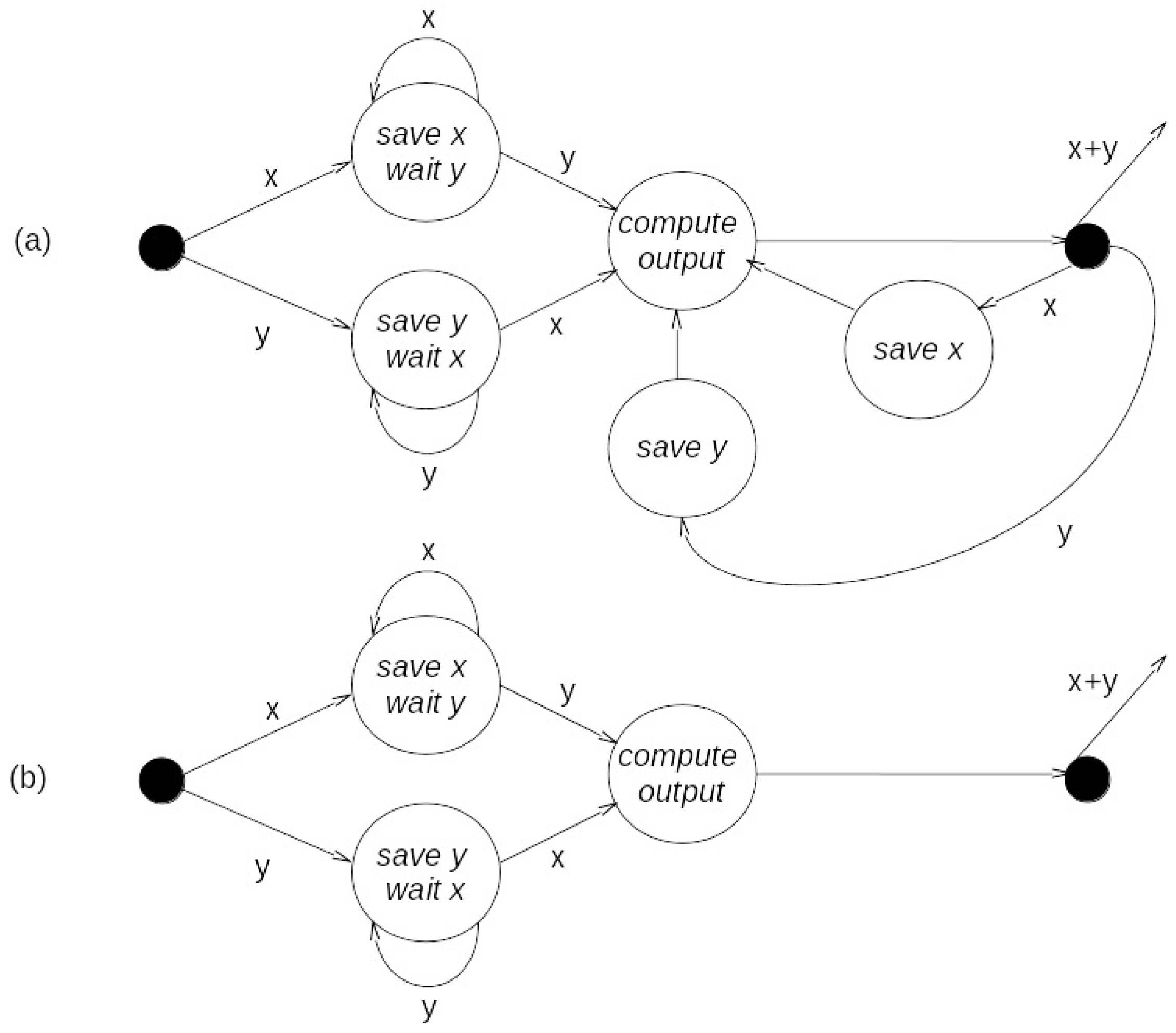
To illustrate the specification of behavior at the I/O level, we consider a simple system—an adder—all it does is add values received on its input ports and transmit their sum as output. However simple this basic adding operation is, there are still many possibilities to consider to characterize its I/O behavior, such as which input values (arriving at different times) are paired to produce an output value, and the order in which the inputs must arrive to be placed in such a pairing. Figure 2 portrays two possibilities, each described as a DEVS model at the I/O system level of the specification hierarchy. In Figure 2a, after the first inputs of contents x and y have arrived, their values are saved, and subsequent inputs refresh these saved values. The output message of content z is generated after the arrival of an input, and its value is the sum of the saved values. In Figure 2b, starting from the initial state, both contents of messages must arrive before an output is generated (from their most recent values), and the system is reset to its initial state after the output is generated. This example shows that even for a simple function, such as adding two values, there can be considerable complexity involved in the specification of behavior when the temporal pattern of the messages bearing such values is considered. Two implications are immediate. One is that there may be considerable incompleteness and/or ambiguity in a semi-formal specification where explicit temporal considerations are often not made. The second implication follows from the first: an approach is desirable to represent the effects of timing in as unambiguous a manner as possible.
3. Systems Implementation of a Memoryless Function
Let be a memoryless function; i.e., it has no time or state dependence [16]. Still, as we have just seen, a system that implements this function may have dynamics and state dependence. Thus, the relationship between a memoryless function and a system that somehow displays that behavior needs to be clearly defined. From the perspective of the hierarchy of systems specifications [16], the relationship involves (1) mapping the input/output behavior of the system to the definition of the function; and (2) working at the state transition level correctly. Additional system specification levels may be brought to bear as needed. Recognizing that the basic relationship is that of simulation between two systems [16], we will keep the discussion quite restricted to limit the complexities.
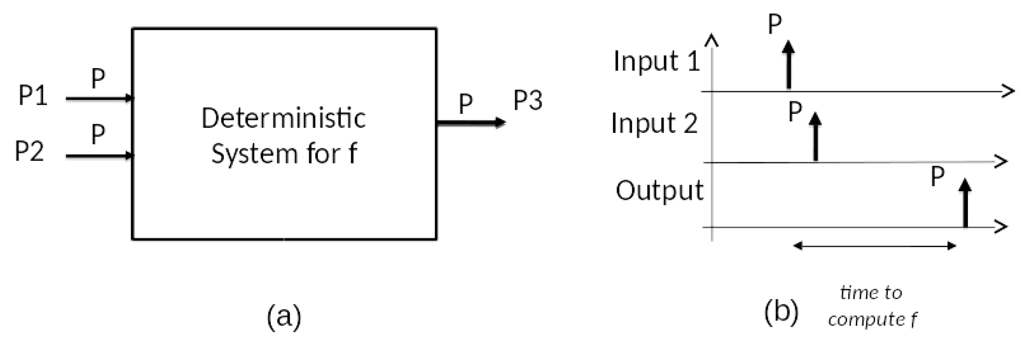
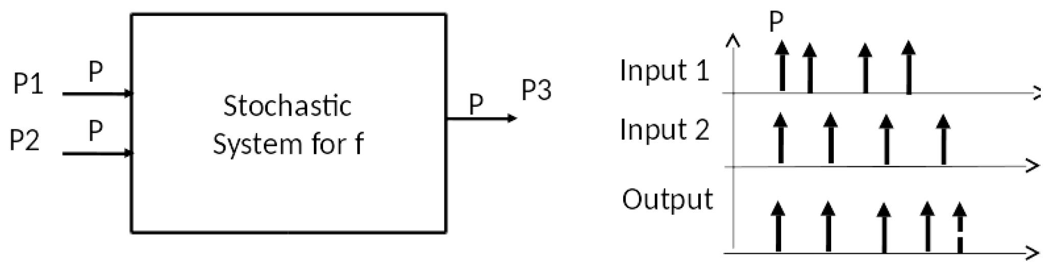
The first thing we need to do is represent the injection of inputs to the function by events arriving to the system. Let us say that the order of the arguments does not count. This is the case for the XOR function. Therefore, we will consider segments of zero, one, or two pulses as input segments, and expect segments of zero or one pulses as outputs. In other words, we are using a very simple decoding of an event segment into the number of events in its time interval. While simplistic, this concept still allows arbitrary event times for the arguments, and therefore consideration of important timing issues. Such issues concern spacing between arguments and time for a computation to be completed. Figure 3 sketches this approach and corresponding deterministic system for f with two input ports P1 and P2 receiving contents P and an output port P3 sending a content P.
Appendix A gives the formal structure of a DEVS basic model, and Appendix B gives our working definition of the simulation relation to be used in the sequel. Having a somewhat formal definition of what it means for a discrete event model to display a behavior equivalent to computing a memoryless function, we turn toward discussing DEVS models that can exhibit such behaviors for the XOR function.
4. DEVS Deterministic Representation of Gelenbe Neuron
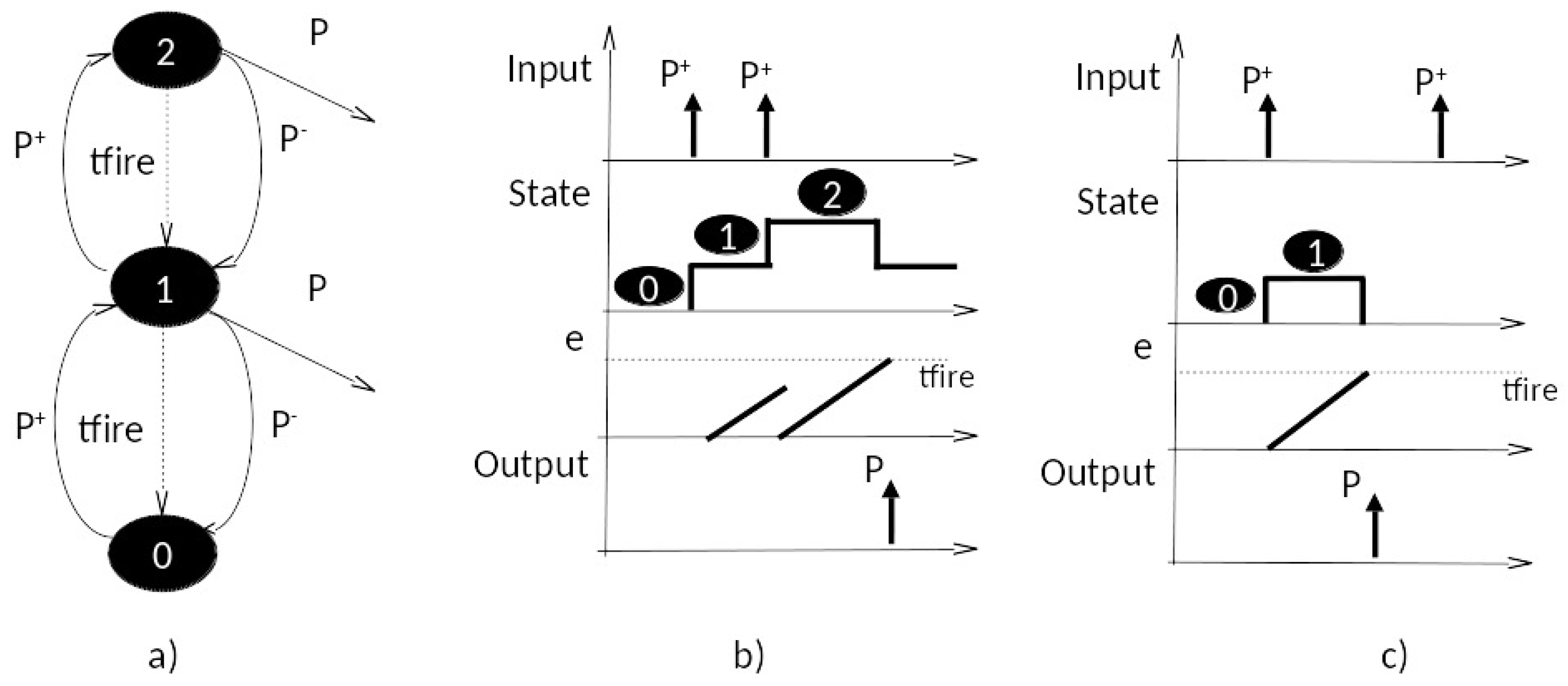
Figure 4a shows a DEVS model that captures the spirit of the Gelenbe stochastic neuron (as shown in [15]) in deterministic form. We first introduce the deterministic model to prepare the ground for discussion of the stochastic neuron in Section 7. Positive pulse arrivals increment the state up to the maximum, while negative pulses decrement the state, stopping at zero. Non-zero states down-transition in a time tfire, a parameter. The DEVS model is given as:
where,
- is the set of positive and negative input pulses,
- is the set of plain pulse outputs,
- is the set of non-negative integer states,
- is the external transition increasing the state by 1 when receiving a positive pulse,
- is the external transition increasing the state by 2 when simultaneously receiving two positive pulses,
- is the external transition decreasing the state by 1 (except at zero) when receiving a negative pulse,
- is the non-zero states internal transition function decreasing the state by one (except at zero),
- is the non-zero states output a pulse,
- is the output sending non-event for states below threshold,
- is the time advance, , for states above 0, and
- is the infinity time advance for zero passive state.
See Appendix A for definitions symbols.
Figure 4b shows an input/state/output trajectory in which two successive positive pulses cause successive increases in the state to 2, which transitions to 1 after tfire, and outputs a pulse. Note that the second positive pulse arrives before the elapsed time has reached tfire, and increases the state. This effectively cancels and reschedules the internal transition back to 0. Figure 4c shows the case where the second pulse comes after firing has happened. Thus, here we have an explicit example of the temporal effects discussed above. Two pulses arriving close enough to each other (within tfire) will effectively be considered as coincident. In contrast, if the second pulse arrives too late (outside the tfire window), it will not be considered as coincident, but will establish its own firing window.
To implement the two logic functions Or and And, we introduce a second parameter into the model—the threshold. Now, states greater or equal to the threshold will transition to zero state in a time tfire and output a pulse. The threshold is set to 1 for the Or, and to 2 for the And function. Thus, any pulse arriving alone is enough to output a pulse for Or, while 2 pulses must arrive to enable a pulse for the And. However, there is an issue with the time advance needed for state 1 in the And case (due to an arrival of a first positive pulse). If this time advance is 0, then there is no time for a second pulse to arrive after a first. If it is infinity, then the model waits forever for a second pulse to arrive. We introduce a third parameter, tdecay, to establish a finite non-zero window after receiving the first pulse for a second one to arrive and be counted as coincident with the first. The revised DEVS model is:
where,
- is the set of positive and negative input pulses,
- is the set of plain pulse outputs,
- is the set of non-negative integer states,
- is the external transition increasing the state by 1 when receiving a positive pulse,
- is the external transition increasing the state by 2 when simultaneously receiving two positive pulses,
- is the external transition decreasing the state by 1 (except at zero) when receiving a negative pulse,
- is the non-zero states internal transition function decreasing the state by one (except at zero),
- is the output sending a pulse for states above or equal threshold,
- is the output sending non-event for states below threshold,
- is the time advance, , for states above or equal threshold, and
- is the time advance, , for states below threshold.
5. Realization of the XOR Function
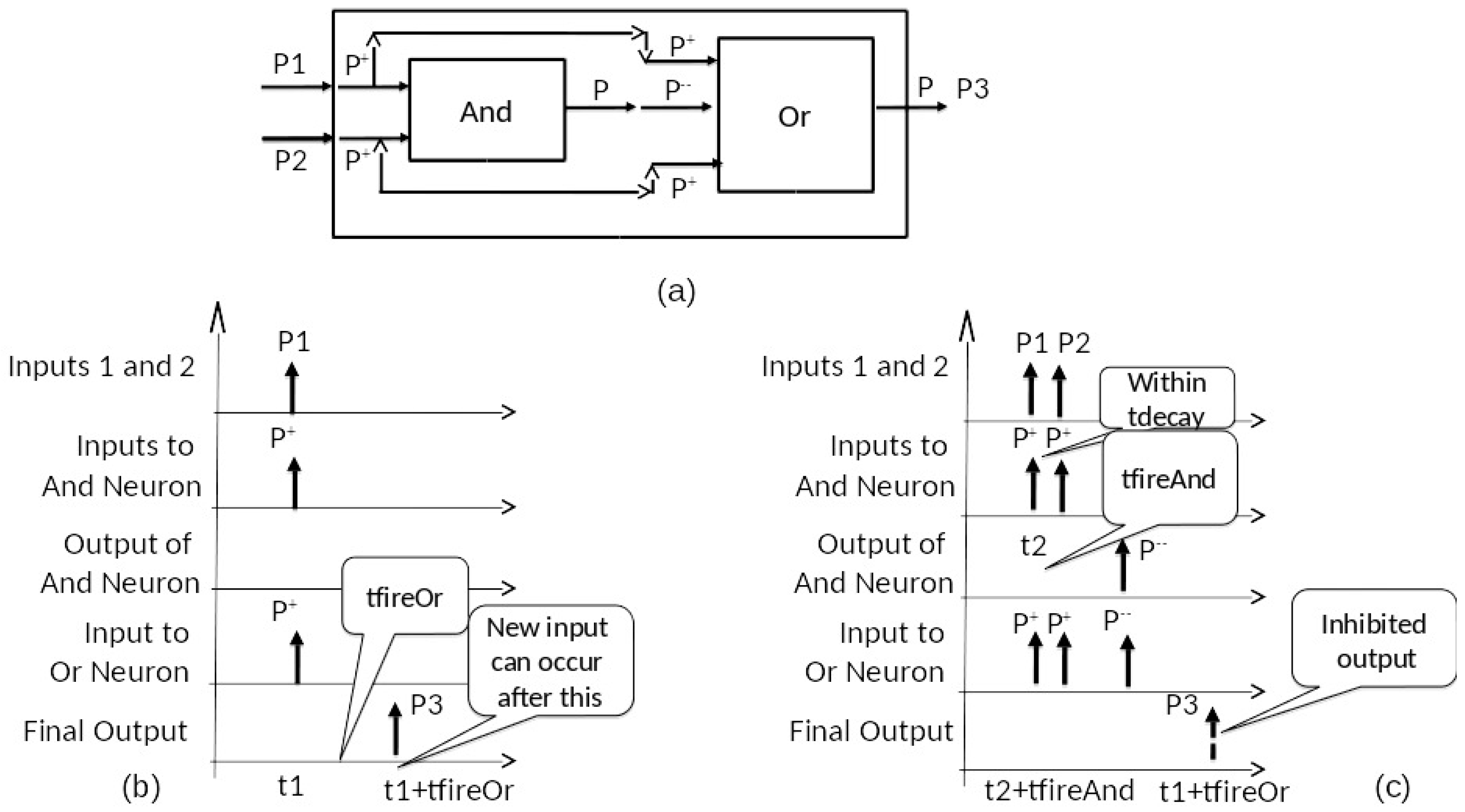
We can use the And and Or models as components in a coupled model, as shown in Figure 5a to implement the XOR function. However as we will see in a moment, we need the response of the And to be slower than that of the Or to enable the correct response to a pair of pulses. So, we let tfireOr and tfireAnd be the time advances of the Or and And response in the above threshold states. As in Figure 5b,c, pulses arriving at the input ports P1 and P2 are mapped in positive pulses by the external coupling that sends them as inputs to both components. When a single pulse arrives within the tdecay window, only the Or responds and outputs a pulse. When a pair of pulses arrive within tdecay window, the And detects them and produces a pulse after tfireAnd. The internal coupling from And to Or maps this pulse into a double negative pulse at the input of the Or. Meanwhile, the Or is holding in State 2 from the pair of positive pulses it has received from the input. So long as the tfireOr is greater than tfireAnd, the double negative pulse will arrive quickly enough to the Or model to reduce its state to zero, thereby suppressing its response. In this way, XOR behavior is correctly realized.
Assertion: The coupled model of Figure 5 with tfireAnd<tfireOr<tdecay realizes the XOR function in the following sense:
- When there are no input pulses, there are no output pulses,
- When a single input pulse arrives and is not followed within tfireAnd by a second pulse, then an output pulse is produced after tfireOr of the input pulse arrival time.
- When the pair of input pulses arrive within tfireAnd of each other, then no output pulse is produced.
Thus, the computation time is tfireOr, since that is the longest time after the arrival of the input arguments (first pulse or second pulse in the pair of pulses case) that we have to wait to see if there is an output pulse. Another metric could also be considered which starts the clock when the first argument arrives, rather than when all arguments arrive.
On the other hand, the time for the system to return to its initial state—and we can send in new arguments for computation—may be longer than the computation time. Indeed, the Or component returns to the zero state after outputting a pulse at tfireOr in both single and double pulse input cases. However, in the first case, the And component—having been put into a non-zero state—only relaxes back to zero after tdecay. Since tdecay is greater than tfireOr, the initial state return time is tdecay.
6. Characterization of SNN I/O Behaviors and Computations
Reference [5] provides a comprehensive review of SNNs, concluding that they have significant potential for solving complicated time-dependent pattern recognition problems because of their inclusion of temporal and dynamic behavior. Maass [11,18,19] and Schmitt [12] characterized third generation SNNs which employ spiking neurons as computational units, accounting for the precise firing times of neurons for information coding, and showed that such networks are computationally more powerful than earlier neural networks. Among other results, they showed that a spiking neuron cannot be simulated by a Boolean network (in particular, a disjunctive composition of conjunctive components with fixed degree). Furthermore, SNNs have the ability to approximate any continuous function [4]. As far as realization of SNN’s in DEVS, the reader may refer to reference [20] for a generic model of a discrete event neuron in an end-to-end nervous system architecture, and to [21] for a complete formal representation of Maass’ SNN from a DEVS simulation perspective. Thus, while there is no question concerning the general ability of SNNs to compute the XOR function, it is of interest to examine the properties of a particular realization—especially one that employs dynamic features that are distinctive to SNNs vice their static neuronal counterparts. Here we draw on the approach of Booij [22], who exhibited an architecture for SNN computation of XOR directly, as opposed to one that relies on the training of a generic net. Like Booij, we change the input and output argument coding to restrict inputs and outputs to particular locations on the timeline. Employing earlier convention, Booij requires inputs to occur at fixed positions, such as either at 0 or 6, and outputs to occur at 10 or 16. Such tight specifications enable a device to be designed that employs synaptic delays and weights to be manipulated to rise above or stay below a threshold, as required. However, the result is highly sensitive to noise, in that any slight change in input position can upset the delicate balancing of delay and weight effects. In contrast, we employ a coding that enables the inputs to have much greater freedom of location while fundamentally employing synaptic delays (although we reduce the essential computation to a static Boolean computation).
As before, we consider the XOR function,
where , .
However, we slightly distinguish the decoding of domain and range. Let specify the decoding of segments to domain of f. Let specify decoding of segments to range of f. With , the I/O function of state q, we require, . In this example, for , we define ω , and ω ; i.e., we require ω .
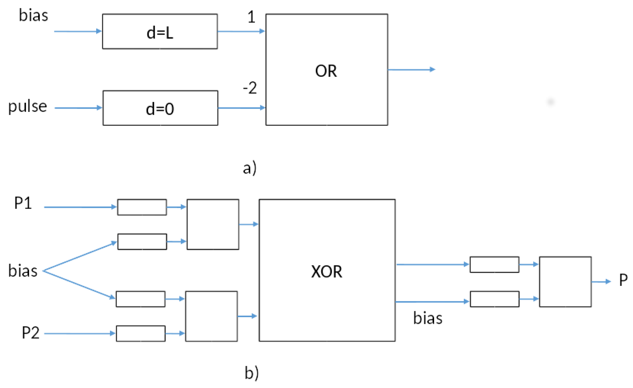
The basic SNN component is shown in Figure 6a, which has two delay elements feeding an OR gate with weights shown. The delay element is behaviorally equivalent to a synaptic delay in an SNN, and is described as DEVS:
where , , , , .
The device rests passively until becoming active when receiving a pulse. It remains active for a time d (the delay parameter), and then outputs a pulse and reverts to passive. The top delay element in Figure 6a has delay, L, and is activated by a bias pulse at time 0 to start the computation. If an input pulse arrives any time before time L, it inhibits the output of the ; otherwise, a pulse is emitted at time L. Thus, the net of Figure 6a can be called an L-arrival detector, since it detects whether a pulse arrives before L and outputs its decision at L. Two such sub-nets are employed in Figure 6b to construct the solution employing SNN equivalent components. After the initial bias, the incoming pulses, and , each arrive early or late relative to L, as detected by the L-detectors. Moreover, any pulses output at the L-arrival detectors are synchronized so that they can be processed by a straightforward gate of the kind constructed earlier (i.e., without concern for timing of arrival). We feed the result into an L-arrival detector in order to report the output back in the form of a pulse that will appear earlier than if we start the output bias at L. Thus, the computation time for this implementation is , and as is its time to resubmission. Indeed, it can function like a computer logic circuit with clock cycle L. Note that unlike Booij’s solution, the solution is not sensitive to exact placement of the pulses, and realistic delays in the gates can be accommodated by delaying the onset of the second bias and reducing the output L-detector’s delay.
7. Probabilistic System Implementation of XOR
Gelenbe’s implementation of the XOR [15] differs quite radically from the deterministic one just given. The concept of what it means for a probabilistic system to realize a memoryless function differs from that given above for a deterministic one.
As illustrated in Figure 7, each argument of the function is represented by an infinite stream of pulses. A stream is modeled as a Poisson stochastic process with a specified rate. An argument value of zero is represented by a null stream (i.e., a rate of zero). We will set the rate equal 1 for a stream representing an argument value of 1. The output of the function is represented similarly as a stream of pulses with a rate representing the value. However, rather than a point, we use an interval on the real line to represent the output value. In the XOR, Gelenbe’s implementation uses an interval to represent 0, with representing 1.
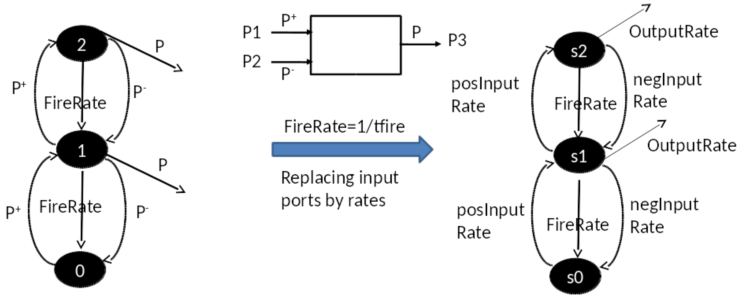
Furthermore, the approach to distinguishing the presence of a single input stream from a pair of such streams—the essence of the problem—is also radically different. The approach formulates the DEVS neuron of Figure 4 as a Continuous Time Markov model (CTM) [17] shown in Figure 8, and exploits its steady state properties in response to different levels of positive and negative input rates. In Figure 8, the CTM on the left has input ports and and output port P. In non-zero states, it transitions to the next lower state with rate FireRate, which is set to the inverse of tfire, interpreted as the mean time advance for such transitions in Figure 4. The Markov Matrix model [17] on the right is obtained by replacing the , and P ports by rates posInputRate and negInputRate, resp. Further, the output port P is replaced by the OutpuRate, which is computed as the FireRate multiplied by the probability of firing (i.e., being in a non-zero state.)
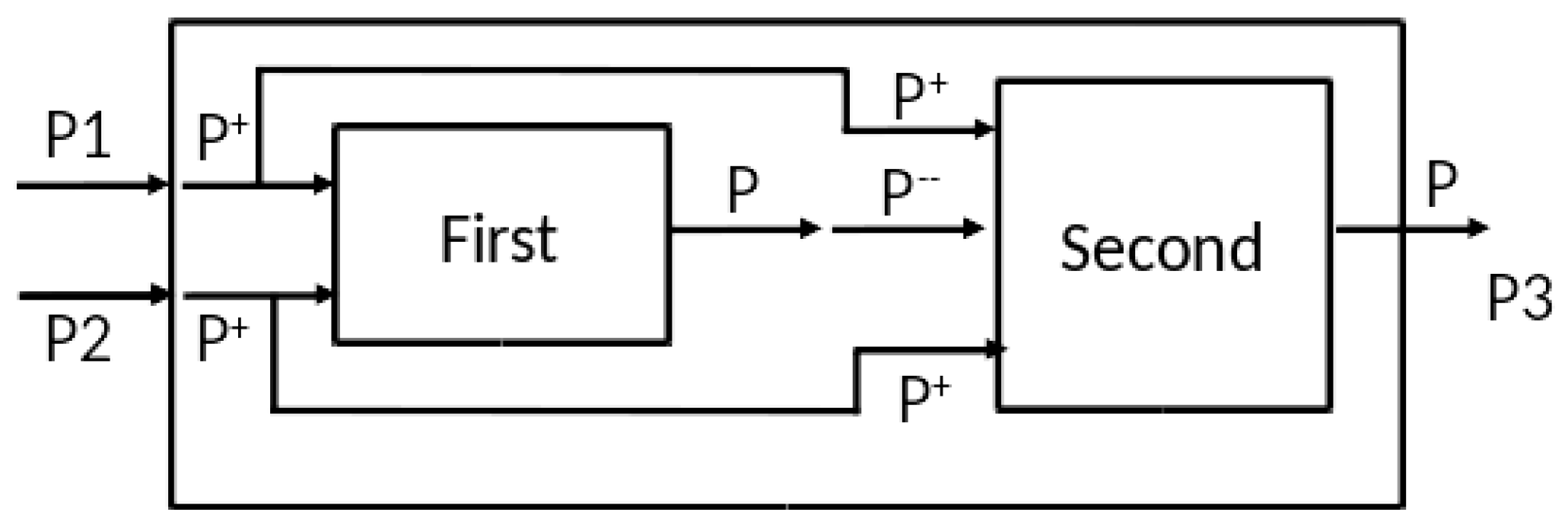
As in Figure 9, each input stream splits into two equal streams of positive and negative pulses by external coupling to two components, each of which is a copy of the CTM model of Figure 8. The difference between the components is that the first component receives only positive pulses, while the second component receives both positive and negative streams. Note that whenever two equal streams with the same polarity converge at a component, they effectively act as a single stream of twice the rate. However, when streams of opposite polarity converge at a component, the result is a little more complex, as we now show.
Now let us consider the two input argument cases. Case 1: one null stream, one non-null stream (representing arguments or ); Case 2: two non-null streams (representing ). In this set-up, Appendix C describes how the first component saturates (fires at its maximum rate) when it receives the stream of positive pulses at either the basic or combined intensities. Therefore, it transmits a stream of positive pulses at the same rate in both Cases 1 and 2. Now, the second component differs from the first in that it receives the (constant) output of the first one. Therefore, it reacts differently in the two cases – its output rate is smaller when the negative pulse input rate is larger (i.e., it is inhibited in inverse relation to the strength of the negative stream). Thus, the output rate is lower in Case 2, when there are two input streams of pulses, than in Case 1, when only one is present. However, since the output rates are not exactly 0 and 1, there needs to be a dividing point (viz., α as above), to make the decision about which case holds. Appendix C shows how α can be chosen so that the output rate of the overall model is below α when two input streams are present, and above α when only one (or none) is present, as required to implement XOR.
8. Discussion
Discussing the proposition of deep neural nets (DNN) as the primary focus of artificial general intelligence, Smith asserts that largely as used, DNNs map vectors to vectors without considering the immediate history of recent inputs nor the time base on which such inputs occur in real counterparts [2]. Note that this is not to minimize the potentially increased ability of relatively simple ANN models to support efficient learning methods [5]. We do not address learnability in this paper. In reality however, time matters because the interplay of the nervous system and the environment occurs via time-varying signals. To be considered seriously as Artificial General Intelligence (AGI), a neural net application will have to work with time-varying inputs to produce time-varying outputs: the world exists in time, and the reaction of a system exhibiting AGI also has to include time [2,23]. Third-generation SNNs have been shown to employ temporal and dynamic properties in new forms of applications that point to such future AGI applications [4,5]. Our results provide a solid system-theoretical foundation and simulation modeling framework for high-performance computational support of such applications.
Although typically considered as deterministic systems, Gelenbe introduced a stochastic model of ANN that provided a markedly different implementation [15]. Based on his use of the XOR logic gate, we formulated definitions for the behavioral realization of memoryless functions, with particular reference to the XOR gate. The definitions of realization turned out to be substantively different for deterministic and stochastic systems constructed of neuron-inspired components. Our definitions of realizations fundamentally include temporal and probabilistic characteristics of their inputs, state, and outputs. Moreover, the realizations of the XOR function that we constructed provide insight into the temporal and probabilistic characteristics that real neural systems might display.
Considering the temporal characteristics of neural nets in relation to functions they implement, we formulated a deterministic DEVS version of Gelenbe’s neural net model, and showed how this model implements the XOR function. Here, we considered timing related to the arrival of pulses, coincidence of pulses, end-to-end time of computation, and time before new inputs can be submitted. We went on to apply the same framework to the realization of memoryless functions by SNNs, illustrating how the formulation allowed for different input/output coding conventions that enabled the computation to exploit the synaptic delay features of SNNs. We then derived a Markov Continuous Time model [17] from the deterministic version, and pointed out the distinct characteristics of the probabilistic system implementation of XOR. We conclude with implications about the characteristics of real-brain computational behaviors suggested by contrasting the ANN perspective and systems-based formulation developed here.
System state and timing considerations we discussed include:
- Time dispersion of pulses—the input arguments are encoded in pulses over a time base, where inter-arrival times make a difference in the output.
- Coincidence of pulses—in particular, whether pulses represent arguments from the same submitted input or subsequent submission depends on their spacing in time.
- End-to-end computation time—the total processing time in a multi-component concurrent system depends on relative phasing as well as component timings, and may be poorly estimated by summing up of individual execution cycles.
- Time for return to ground state—the time that must elapse before a system that has performed a computation is ready to receive new inputs may be longer than its computation time, as it requires all components to return to their ground states.
Although present in third-generation models, system state and timing considerations are abstracted away by neural networks typified by DNNs that are idealizations of intelligent computation; consequently, they may miss the mark in two aspects:
- As static recognizers of memoryless patterns, DNNs may become ultra-capable (analogous to AlphaGo progress [24]), but as representative of human cognition, they may vastly overemphasize that one dimension and correspondingly underestimate intelligent computational capabilities in humans and animals in other respects.
- As models of real neural processing, DNNs do not operate within the system temporal framework discussed here, and therefore may prove impractical in real-time applications which impose time and energy consumption constraints such as those just discussed [25].
It is instructive to compare the computation-relevant characteristics of the deterministic and stochastic versions of the DEVS neuron models we discussed. The deterministic version delivers directly interpretable outputs within a specific processing time. The Gelenbe stochastic version formulates inputs and outputs as indefinitely extending streams modelled by Poisson processes. Practically speaking, obtaining results requires measurement over a sufficiently extended period to obtain statistical validity and/or to enable a Bayesian or Maximum Likelihood detector to make a confidence-dependent decision. On the other hand, a probabilistic version of the DEVS neuron can be formulated that retains the direct input/output encoding, but can also give probability estimates for erroneous output. Some of these models have been explored [9,21], while others explicitly connecting to leaky integrate-and-fire neurons are under active investigation [26]. Possible applications of DEVS modeling to the extensive literature on Gelenbe networks are considered in Appendix D. Along these lines, we note that both the deterministic and probabilistic implementations of XOR use the negative inputs in an essential (although different) manner to identify the input argument and inhibit the output produced when it occurs (note that the use of negative synaptic weights is also essential in the SSN implementation, although in a somewhat different form). This suggests research to show that XOR cannot be computed without use of negative inputs, which would establish a theoretical reason for why inhibition is fundamentally needed for leaky integrate-and-fire neuron models—a reason that is distinct from the hidden layer requirement uncovered by Rumelhart [7].
Although not within the scope of this paper, the DEVS framework for I/O behavior realization would seem to be applicable to the issue of spike coding by neurons. A reviewer pointed to the recent work of Yoon [27], which provides new insights by considering neurons as analog-to-digital converters. Indeed, encoding continuous-time signals into spikes using a form of sigma-delta modulation would fit the DEVS framework which accommodates both continuous and discrete event segments. Future research could seek to characterize properties of I/O functions that map continuous segments to discrete event segments [16,20].
Author Contributions
B.P. Zeigler developed the different models in interaction with Alexandre Muzy who provided his expertise in mathematical system-theory and neural net modeling.
Conflicts of Interest
The authors declare no conflict of interest.
Appendix A. Discrete Event System Specification (DEVS) Basic Model
A basic Discrete Event System Specification (DEVS) is a mathematical structure
where X is the set of input events, Y is the set of output events, S is the set of partial states, is the external transition function with the set of total states with e the elapsed time since the last transition, is the internal transition function, is the output function, and is the time advance function.
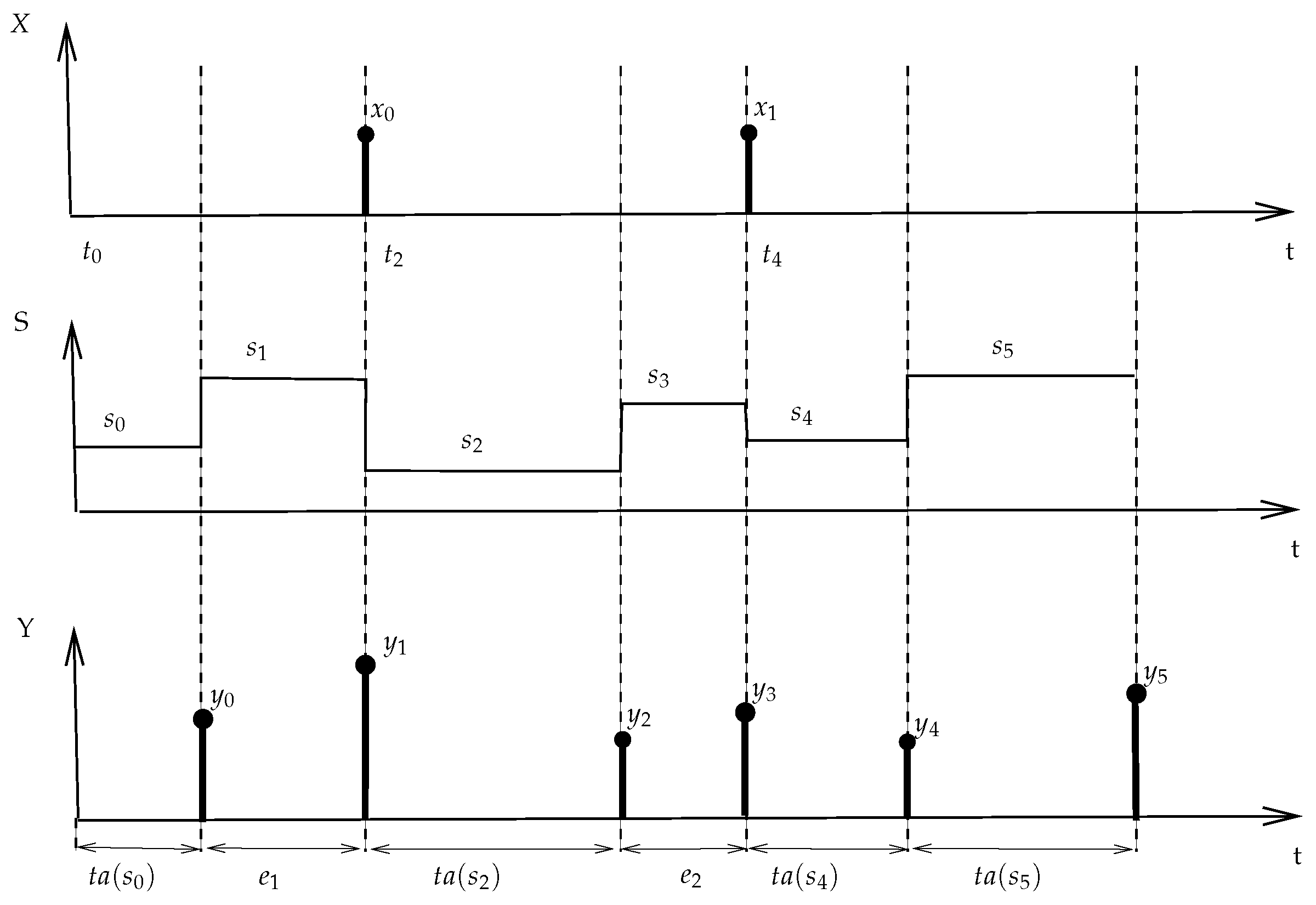
Figure A1 depicts simple trajectories of a DEVS. The latter starts in initial state at time , and schedules an internal event occurring after time advance , where value is output, and state changes to . At time , an external event of value occurs, changing the state to with the elapsed time since the last transition. Then, an internal event is scheduled at time advance , and so on.
Figure A1.
Simple DEVS trajectories.

Appendix B. Simulation Relation
Consider a function having the same domain and range,
For example, an XOR function where , . Let,
That is, specify decoding of segments to domain and range of f. Let
be the I/O Function of state q mapping input segments to output segments.
If , we require ; i.e., input segment ω mapped to output segment ρ when decoded is required to satisfy f. That is, . Applying the requirement to DEVS segments of pulses, let ; i.e., = number of pulses in ω requiring . That is, number of pulses in .
Appendix C. Behavior of the Markov Model
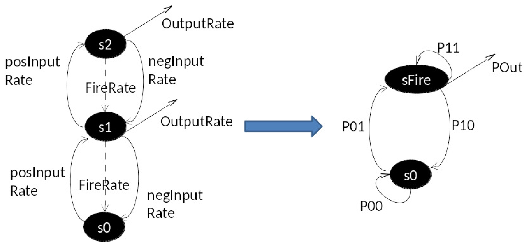
We first reduce the infinite state Matrix model to a two-state version that is equivalent with respect to the output pulse rate in steady state. As in Figure C1, all the non-zero states are lumped into a single firing state, sFire, and we will interpret each of the probabilities in terms of the original rates as follows:
- There is only one way to transition from s0 to sFire, and that is by going from s0 to s1 in the original model, which happens with posInputRate. Therefore, .
- Similarly, there is only one way to transition from sFire to s0, and this happens with . Therefore, .
- The probability of remaining in the sFire, (these must sum to 1).
- Similarly, .
Figure C1.
Reduction to two-state Markov Matrix model.
Now, in the reduced model, the steady state probabilities are easy to compute in terms of the transition probabilities. Indeed, the probability of being in the firing state, for .
Additionally, the rate of producing output pulses
The case of saturation occurs when the positive input rate is “very large" compared to the rates that lower the state, especially when the negative input rate is 0, so that and .
Thus, the output of the first component saturates at the maximum, FireRate. This is input to the second component so that we have for it:
So, we see that the output rate is inversely related to the negative pulse input which, by design, the second component receives, but not the first.
Appendix D. Possible Applications of DEVS Modeling to Random Neural Networks
Random neural network (RNN)—a probabilistic model inspired by neuronal stochastic spiking behavior—have received much examination. Here we focus on two main extensions: synchronous interaction and spike classes. Gelenbe developed an extension of the RNN [28,29,30,31,32,33] to the case when synchronous interactions can occur, modeling synchronous firing by large ensembles of cells. Included are recurrent networks having both conventional excitatory–inhibitory interactions and synchronous interactions. Although modeling the ability to propagate information very quickly over relatively large distances in neuronal networks, the work focuses on developing a related learning algorithm. Synchronous interactions take the form of a joint excitation by a pair of cells on a third cell. One can assign as the probability that when cell i fires, then if cell j is excited, it will also fire immediately, with an excitatory spike being sent to cell m. This synchronous behavior can be extended to an arbitrary number of cells that can simultaneously fire. DEVS modeling includes zero time advance possibility to capture such behavior, as was illustrated in application to physical action-at-a-distance by Zeigler [14]. The standard RNN approach has been concerned with equilibrium analysis, and it may be interesting to see how the DEVS equivalent modeling can throw light on the plausibility of such zero time advances and any difference they would make in the temporal I/O behavior of interest to us here.
RNNs with multiple spike classes of signals were introduced to represent interconnected neurons which simultaneously process multiple streams of data, such as the color information of images or networks which simultaneously process streams of data from multiple sensors. One network was used to generate a synthetic texture that imitates the original image. To exchange spikes of different types, neurons have potentials that generate corresponding excitatory spikes in a manner similar to the single potential case. Inhibitory spikes are of only one type, and affect class potential in proportion to their levels. DEVS models can represent such neurons, but there seems to be no evidence for biological plausibility of such a structure. It would be interesting to see if the structure and behavior manifested by multi-class RNNs can be realized by groups of ordinary neurons in the roles of spike processing classes; e.g., interacting cell assemblies specifically tuned to red, green, and blue color wavelengths.
References
- Carandini, M. From circuits to behavior: A bridge too far? Nat. Neurosci. 2012, 15, 507–509. [Google Scholar] [CrossRef] [PubMed]
- Smith, L.S. Deep neural networks: The only show in town? In Proceeedings of the Workshop on Can Deep Neural Networks (DNNs) Provide the Basis for Articial General Intelligence (AGI) at AGI 2016, New York, NY, USA, 16–19 July 2016.
- Goertzel, B. Are There Deep Reasons Underlying the Pathologies of Today’s Deep Learning Algorithms? In Artificial General Intelligence; Springer International Publishing: Cham, Switzerland, 2015; pp. 70–79. [Google Scholar]
- Paugam-Moisy, H.; Bohte, S. Computing with Spiking Neuron Networks. In Handbook of Natural Computing; Kok, J., Heskes, T., Eds.; Springer: Berlin/Heidelberg, Germany, 2009. [Google Scholar]
- Ghosh-Dastidar, S.; Hojjat, A. Spiking neural networks. Int. J. Neural Syst. 2009, 19, 295–308. [Google Scholar] [CrossRef] [PubMed]
- Minsky, M.; Papert, S. Perceptrons; MIT Press: Cambridge, MA, USA, 1969. [Google Scholar]
- Rumelhart, D.E.; Hinton, G.E.; Williams, R.J. Parallel Distributed Processing: Explorations in the Microstructure of Cognition. Vol. 1: Foundations; Rumelhart, D.E., McClelland, J.L., Eds.; MIT Press: Cambridge, MA, USA, 1986; pp. 318–362. [Google Scholar]
- Bland, R. Learning XOR: Exploring the Space of a Classic Problem; Computing Science Technical Report; Department of Computing Science and Mathematics, University of Stirling: Stirling, Scotland, June 1998. [Google Scholar]
- Toma, S.; Capocchi, L.; Federici, D. A New DEVS-Based Generic Artificial Neural Network Modeling Approach. In Proceedings of the EMSS 2011, Rome, Italy, 12 September 2011.
- Pessa, E. Neural Network Models: Usefulness and Limitations. In Nature-Inspired Computing: Concepts, Methodologies, Tools, and Applications; IGI Global: Hershey, PA, USA, 2017; pp. 368–395. [Google Scholar]
- Maass, W. Lower bounds for the computational power of spiking neural networks. Neural Comput. 1996, 8, 1–40. [Google Scholar] [CrossRef]
- Schmitt, M. On computing Boolean functions by a spiking neuron. Ann. Math. Artif. Intell. 1998, 24, 181–191. [Google Scholar] [CrossRef]
- Brette, R.; Rudolph, M.; Carnevale, T.; Hines, M.; Beeman, D.; Bower, J.M.; Diesmann, M.; Morrison, A.; Goodman, P.H.; Harris, F.C., Jr.; et al. Simulation of networks of spiking neurons: A review of tools and strategies. J. Comput. Neurosci. 2007, 23, 349–398. [Google Scholar] [CrossRef] [PubMed]
- Zeigler, B.P. Cellular Space Models: New Formalism for Simulation and Science. In The Philosophy of Logical Mechanism: Essays in Honor of Arthur W. Burks; Salmon, M.H., Ed.; Springer: Dordrecht, The Netherlands, 1990; pp. 41–64. [Google Scholar]
- Gelenbe, E. Random Neural Networks with Negative and Positive Signals and Product Form Solution. Neural Comput. 1989, 1, 502–510. [Google Scholar] [CrossRef]
- Zeigler, B.P.; Kim, T.G.; Praehofer, H. Theory of Modeling and Simulation: Integrating Discrete Event and Continuous Complex Dynamic Systems, 2nd ed.; Academic Press: Boston, MA, USA, 2000. [Google Scholar]
- Zeigler, B.P.; Nutaro, J.; Seo, C. Combining DEVS and Model-Checking: Concepts and Tools for Integrating Simulation and Analysis. Int. J. Process Model. Simul. 2016, in press. [Google Scholar]
- Maass, W. Fast sigmoidal networks via spiking neurons. Neural Comput. 1997, 9, 279–304. [Google Scholar] [CrossRef] [PubMed]
- Maass, W. Networks of Spiking Neurons: The Third Generation of Neural Network Models. Neural Netw. 1996, 10, 1659–1671. [Google Scholar] [CrossRef]
- Zeigler, B.P. Discrete Event Abstraction: An Emerging Paradigm For Modeling Complex Adaptive Systems. In Perspectives on Adaptation in Natural and Artificial Systems; Booker, L., Forrest, S., Mitchell, M., Riolo, R., Eds.; Oxford University Press: New York, NY, USA, 2005; pp. 119–141. [Google Scholar]
- Mayerhofer, R.; Affenzeller, M.; Fried, A.; Praehofer, H. DEVS Simulation of Spiking Neural Networks. In Proceedings of the Euro-Pean Meeting on Cybernetics and Systems, Vienna, Austria, 30 March–1 April 2002.
- Booij, O. Temporal Pattern Classification using Spiking Neural Networks. Master’s Thesis, Universiteit van Amsterdam, Amsterdam, The Netherlands, August 2004. [Google Scholar]
- Maass, W.; Natschlager, T.; Markram, H. Real-time computing without stable states: A new framework for neural computation based on perturbations. Neural Comput. 2002, 14, 2531–2560. [Google Scholar] [CrossRef] [PubMed]
- Koch, C. How the Computer Beat the Go Master, Scientific American. 2016. Available online: https://www.scientificamerican.com/article/how-the-computer-beat-the-go-master/ (accessed on 14 January 2017).
- Hu, X.; Zeigler, B.P. Linking Information and Energy—Activity-based Energy-Aware Information Processing. Simul. Trans. Soc. Model. Simul. Int. 2013, 89, 435–450. [Google Scholar] [CrossRef]
- Muzy, A.; Zeigler, B.P.; Grammont, F. Iterative Specification of Input-Output Dynamic Systems and Implications for Spiky Neuronal Networks. IEEE Syst. J. 2016. Available online: http://www.i3s.unice.fr/muzy/Publications/neuron.pdf (accessed on 14 January 2017). [Google Scholar]
- Yoon, Y.C. LIF and Simplified SRM Neurons Encode Signals Into Spikes via a Form of Asynchronous Pulse Sigma-Delta Modulation. IEEE Trans. Neural Netw. Learn. Syst. 2016, PP, 1–14. [Google Scholar] [CrossRef] [PubMed]
- Gelenbe, E. G-networks: A unifying model for neural and queueing networks. Ann. Oper. Res. 1994, 48, 433–461. [Google Scholar] [CrossRef]
- Gelenbe, E.; Fourneau, J.M. Random Neural Networks with Multiple Classes of Signals. Neural Comput. 1999, 11, 953–963. [Google Scholar] [CrossRef] [PubMed]
- Gelenbe, E. The first decade of G-networks. Eur. J. Oper. Res. 2000, 126, 231–232. [Google Scholar] [CrossRef]
- Gelenbe, E. G-networks: Multiple classes of positive customers, signals, and product form results. In IFIP International Symposium on Computer Performance Modeling, Measurement and Evaluation; Springer: Berlin/Heidelberg, Germany, 2002. [Google Scholar]
- Gelenbe, E.; Timotheou, S. Random Neural Networks with Synchronized Interactions. Neural Comput. 2008, 20, 2308–2324. [Google Scholar] [CrossRef] [PubMed]
- Gelenbe, E.; Timotheou, S. Synchronized Interactions in Spiked Neuronal Networks. Comput. J. 2008, 51, 723–730. [Google Scholar] [CrossRef]
Figure 1.
Representing an input/output pair.
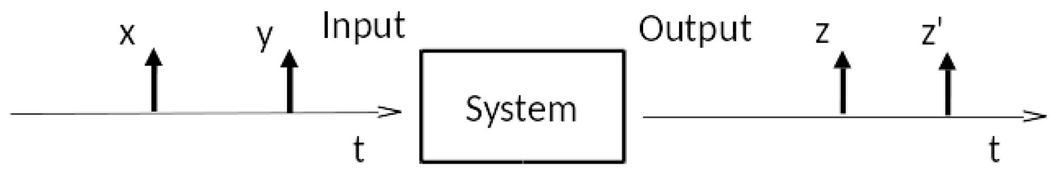
Figure 2.
Variants of behavior and corresponding input/output (I/O) pairs, with (a) saving input values when they arrived; or (b) resetting to initial state once the output is computed. White circles indicate states, black circles initial states, and arrows transitions.
Figure 2.
Variants of behavior and corresponding input/output (I/O) pairs, with (a) saving input values when they arrived; or (b) resetting to initial state once the output is computed. White circles indicate states, black circles initial states, and arrows transitions.

Figure 3.
Deterministic system realization of memoryless function: (a) Input/Output Black Box; (b) Input and Output Trajectories.
Figure 3.
Deterministic system realization of memoryless function: (a) Input/Output Black Box; (b) Input and Output Trajectories.

Figure 4.
Two-state deterministic Discrete Event System Specification (DEVS) model of Gelenbe neuron, with (a) DEVS state graph; (b) Closely Spaced Inputs; and (c) Widely Spaced Inputs. The time elapsed since the last transition is indicated as .
Figure 4.
Two-state deterministic Discrete Event System Specification (DEVS) model of Gelenbe neuron, with (a) DEVS state graph; (b) Closely Spaced Inputs; and (c) Widely Spaced Inputs. The time elapsed since the last transition is indicated as .

Figure 5.
Coupled Model for XOR Implementation, with (a) XOR Network Description; (b) Single Input Pulse; and (c) Double Input Pulse. Note that t1 in (c) is the same time in (b), representing the time an inhibited pulse would have arrived.
Figure 5.
Coupled Model for XOR Implementation, with (a) XOR Network Description; (b) Single Input Pulse; and (c) Double Input Pulse. Note that t1 in (c) is the same time in (b), representing the time an inhibited pulse would have arrived.

Figure 6.
Implementation of the XOR using Spiking Neural Net (SNN) equivalent components described in DEVS: (a) L-Arrival Component; (b) XOR Coupled Model.
Figure 6.
Implementation of the XOR using Spiking Neural Net (SNN) equivalent components described in DEVS: (a) L-Arrival Component; (b) XOR Coupled Model.

Figure 7.
Stochastic system realization of a memoryless function.

Figure 8.
Mapping DEVS Neuron Continuous Time Markov (CTM) model to Markov Matrix model.

Figure 9.
Stochastic coupled model implementation of XOR.

© 2017 by the authors. Licensee MDPI, Basel, Switzerland. This article is an open access article distributed under the terms and conditions of the Creative Commons Attribution (CC BY) license ( http://creativecommons.org/licenses/by/4.0/).
Share and Cite
MDPI and ACS Style
Zeigler, B.P.; Muzy, A. Temporal Modeling of Neural Net Input/Output Behaviors: The Case of XOR. Systems 2017, 5, 7. https://doi.org/10.3390/systems5010007
AMA Style
Zeigler BP, Muzy A. Temporal Modeling of Neural Net Input/Output Behaviors: The Case of XOR. Systems. 2017; 5(1):7. https://doi.org/10.3390/systems5010007
Chicago/Turabian StyleZeigler, Bernard P., and Alexandre Muzy. 2017. "Temporal Modeling of Neural Net Input/Output Behaviors: The Case of XOR" Systems 5, no. 1: 7. https://doi.org/10.3390/systems5010007
Note that from the first issue of 2016, this journal uses article numbers instead of page numbers. See further details here.