Article

Case Study for the Return on Investment of Internet of Things Using Agent-Based Modelling and Data Science

1
Department of Aeronautics, Imperial College London, South Kensington Campus, London SW7 2AZ, UK
2
Amey Strategic Consulting and Technology, 10 Furnival Street, London EC4A 1AB, UK
*
Author to whom correspondence should be addressed.
Submission received: 25 October 2016 / Revised: 21 December 2016 / Accepted: 12 January 2017 / Published: 25 January 2017

Abstract

:
As technology advances towards new paradigms such as the Internet of Things, there is a desire among business leaders for a reliable method to determine the value of supporting these ventures. Traditional simulation and analysis techniques cannot model the complex systems inherent in fields such as infrastructure asset management, or suffer from a lack of data on which to build a prediction. Agent-based modelling, through an integration with data science, presents an attractive simulation method to capture these underlying complexities and provide a solution. The aim of this work is to investigate this integration as a refined process for answering practical business questions. A specific case study is addressed to assess the return on investment of installing condition monitoring sensors on lift assets in a London Underground station. An agent-based model is developed for this purpose, supported by analysis from historical data. The simulation results demonstrate how returns can be achieved and highlight features induced as a result of stochasticity in the model. Suggestions of future research paths are additionally outlined.

1. Introduction

How do you reliably assess the business value of new technologies in the absence of real-world cases? This question has become increasingly relevant in recent years as technologies continue to develop at a rapid pace and businesses have a desire to utilise them in the most effective way to fulfil their strategic objectives. The current work seeks to extend recent research in the fields of agent-based modelling and data science to investigate a framework for determining the return on investment of new ventures such as the Internet of Things and Smart Cities, applied within the scope of infrastructure asset management.
With technological trends like the Internet of Things and Smart Cities beginning to emerge following the recent ascension of Big Data, businesses could benefit from understanding how to enhance their performance through realising the greatest value from investments in these technologies. However, as they are new phenomena, there is a lack of historical data and real business cases regarding their implementation and subsequent returns. Traditional techniques for estimating potential return on investment fall short of providing an answer. This is slowing the uptake of technology that could lead to significant advances in fields such as infrastructure asset management and, beyond business, the living standards of the general population.
The aim of this research is to investigate an integration of agent-based modelling and data science as a practical solution to this problem, applied in particular to the theme of infrastructure asset management. Agent-based modelling is a simulation method with roots in complexity science and is used to provide understanding and predictive capabilities in environments with many interacting entities. Data science is a wide field focused on deriving quantitative and qualitative insight from datasets and encompasses many potential applications. Both of these fields can offer answers but are hindered by their respective disadvantages. Through combining them, it is possible to alleviate some of their individual limitations and reinforce their results. Infrastructure asset management is also a large subject with the general objective of deriving value from an organisation’s assets. Hereafter, any use of the term asset management refers to infrastructure asset management unless stated otherwise.
The rest of this paper is structured as follows. After this introduction, Section 2 covers background information to this research through an extensive literature review in each key field, as well as examples of agent-based models developed with similar features or motivations to the current research. Section 3 builds on insights from the literature review to specify the particular case study addressed in this work. Practical considerations to this case are discussed in Section 4. Following that, a detailed description of the developed agent-based model is provided in Section 5, including the validation process. Finally, Section 6 presents the obtained results and a critical discussion before the paper is concluded in Section 7.

2. Literature Review

2.1. Asset Management

The International Organization for Standardization (ISO) [1] defines Asset Management as the ‘coordinated activity of an organization to realise value from assets’ (p. 14). They define an Asset as an ‘item, thing or entity that has potential or actual value to an organization’ (p. 2). These are clearly general definitions and apply to many organisations which may not previously have been considered to involve asset management processes. Indeed, assets may be financial, human or physical in nature. The effective management of assets is a crucial requirement for organisations to realise their strategic objectives and achieve their stakeholders’ expectations [2]. While the standards can be applied to any form of asset management, this work will focus in particular on their application to the management of infrastructure assets.
In 2014, the ISO 55000 series [1,3,4] was released as a development upon the previous PAS 55 standards. This represents the first international asset management standard that attempts to capture the general terminology, requirements and methodology for successful asset management. The Institute of Asset Management also released a comprehensive guide on the application of the standards [2] through which they discuss the 39 key areas in the field. These recent developments highlight the importance of asset management to businesses and society in general, driven by the emerging areas of promising technology that could revolutionise the way we live our lives.

2.1.1. Internet of Things and Smart Cities

IBM, in a 2013 report on big data in smart infrastructures [5], identify four key ways through which the utilisation of Big Data can be beneficial to asset management. Firstly, by boosting generated revenue through more effective decision-making from a deeper understanding of the information affecting a firm. Secondly, by allowing a company to increase its operational efficiency by optimising many of its common processes. Thirdly, by realising optimal maintenance strategies throughout an asset’s life cycle via monitoring and benchmarking techniques. Lastly, and perhaps most importantly, by reducing risk through the application of predictive analytics to understand failure patterns of assets in order to carry out more effective maintenance.
The Internet of Things (IoT) is an emerging concept in wireless communications whereby vast numbers of commonplace items throughout the world can be augmented with sensors and microcontrollers that will enable them to interact with each other and users, resulting in a completely immersive internet [6]. The Smart City paradigm is the application of the IoT within an urban context that will allow asset management firms to manage infrastructure in a city environment more effectively, thereby increasing citizen satisfaction and reducing operational costs [7].
The IoT is estimated to have potential to generate total value of $14.4 trillion in the private sector in future years (given in a Cisco 2013 IoE Value Index Study) with the likely prospect of over 50 billion devices connected to the internet by 2020 [8]. However its general uptake is currently hindered by a lack of clear returns on the initial and ongoing technology investments. A recent World Economic Forum report [9] stated uncertain return on investment due to a lack of real-world business cases as the third largest barrier to the uptake of the IoT, closely following lack of standards and security concerns. Whereas paths to alleviate the two largest problems exist, there is no clear solution for deriving a reliable business value from these ventures. This is critical if business leaders are to enthusiastically adopt the technologies.

2.1.2. Return on Investment

Business leaders in infrastructure asset management rely on metrics to assess their options and make decisions. Return on Investment (RoI) is a key metric to assess the performance of an investment strategy and compare it to alternatives [10,11]. Traditional RoI determines the efficiency of an investment through cost savings (or revenue gains), and is usually given in percentage form by Equation (1).
RoI = Cost savings Investment Investment
For effective calculation of the RoI of a project, it is imperative to understand which savings can be attributed to its implementation as well as how to determine the size of investment required. The Investment value in Equation (1) is typically easier to predict than the Cost savings value as investments are normally monetary in nature, can be easily quantified and are generally known as they predominantly occur at the outset of the project. In comparison, for established endeavours, it is common to use empirical equations based on assumptions derived from past experience to estimate cost savings [12]. However, as was noted above, it is much more difficult to assess the tangible and intangible benefits from emerging paradigms such as the IoT and Smart Cities where there is a lack of historical data.
Due to the typical long-term nature of returns in organisational investments, it is often necessary to calculate the discounted RoI rather than the traditional form [10,13]. Future returns are generally considered to be worth less than the present due to the increasing uncertainty involved as they extend forward in time. To account for this, they are discounted to their present values [10,13]. A standard discount rate often exists within organisations for these calculations.
Figures that can be used in calculation of RoI are not solely monetary. Key Performance Indicators (KPIs) are commonly employed to measure gains and losses by attaching value to an activity’s success. They are an important aspect of monitoring the effectiveness of strategies in infrastructure asset management firms [14,15]. KPIs are typically chosen specific to a firm’s activities. As an example, asset managers in Transport for London (TfL) use Lost Customer Hours, representing customers’ time wasted due to service problems and delays, to measure the impact of disruptions throughout their network.
Currently, standard analysis and prediction processes are used by asset management firms in understanding the impact of business decisions. Traditional forecasting methods, such as moving averages, can be utilised to predict the future trend of variables given their past performance [16]. Game theoretical techniques can also be employed to support strategy and decision-making. Game theory is the analysis of decision-making between players in the game of business that takes into account interactions as well as benefits and costs [17]. While it requires logical thinking rather than a wealth of data to use, its main limitation comes from one of its key pillars: that all players must act rationally. This behaviour leads to a potential oversight in business strategy as sometimes irrational behaviour is a more appropriate representation of reality [18]. Additionally, game theory is often misused to provide an overly accurate, single answer to complex problems [19].
Despite the lack of historical data, a few attempts have been made to characterise a process for assessing the value of IoT and Smart Cities to business [20]. However, these tend to adopt a qualitative approach to the topic which makes it difficult to provide a solid foundation for a RoI value.

2.1.3. Asset Maintenance

The effective maintenance of physical assets is a key aspect of infrastructure asset management. There are two broad categories of maintenance in this context: emergency (also known as corrective, reactive or run-to-failure) and planned (also known as preventative) [21,22]. In practise, it is possible to differentiate between all these maintenance tasks, for example corrective maintenance is not necessarily "emergency" and can include remedial action due to issues identified during preventive maintenance activities that could potentially result in failure (emergency and corrective could be categorised as "reactive"). Similarly, a "run-to-failure" approach should be only implemented in very specific circumstances because it can cause secondary damage to other components, for example through excessive vibration or temperature, which can result in higher repair costs and more downtime. For the sake of simplicity the present study will assume only emergency and planned maintenance tasks.
Emergency maintenance is carried out post-failure whereas planned maintenance is scheduled in advance in an effort to reduce the chance of failure occurring. Planned maintenance is a time-driven process. Standard methods involve carrying out services on assets at regular intervals based on an assumed asset failure behaviour. In this way, the maintenance can be carried out at a time of day when it does not affect the operation of the asset [21].
Predictive maintenance (also known as condition-based maintenance) is a form of planned maintenance that makes use of condition monitoring to determine when repairs are required. Measurements of specific variables (e.g., heat, vibration) are taken frequently during operation of the asset. The collected data can then be analysed to estimate its current condition and the information used to decide when maintenance tasks should be carried out [11,23]. This dynamic form of planned maintenance contrasts the static form where maintenance policies have been set up prior to the asset entering service.
For predictive maintenance solutions, the most direct and apparent saving is usually the reduced overall cost of maintenance [11]. Emergency maintenance procedures can be four times as expensive as planned work due to the requirement for engineers to be on call and the necessary quick response time [22]. As such, any reduction in their frequency can represent a substantial saving. Generally, an effective predictive maintenance strategy will also lead to reduced asset time out of service. This brings significant, though less visible, indirect cost savings.
As a result of the IoT, it is now more cost effective to install remote sensors on physical assets to provide continuous real-time data and enable predictive maintenance. These sensors are typically connected in a distributed arrangement known as a Wireless Sensor Network (WSN) [24,25]. Each sensor node generally consists of the monitoring technology (such as thermometers or accelerometers), a means of communication (such as a radio transceiver), a power source (typically batteries) and a microcontroller [25]. There are initial and ongoing costs related to the application of these solutions within industry [26]. The initial investment is generally composed of the cost of the hardware and the installation process. Ongoing costs are related to sensor upkeep (e.g., recharging batteries) as well as data collection and storage.

2.1.4. Failure Probability

Insight into an asset’s changing probability of failure over time is essential in order to reduce the risk of unnecessary time out of service. In the field of reliability engineering, a number of key concepts exist for evaluating the likelihood of asset failures [21,27] and are summarised below.
Firstly, if we let t = 0 be the time at which an asset is considered new, then the random variable depicting failure time t = T may be described by a cumulative distribution function, F ( t ) . This gives the probability that an asset will fail before or at time t. The probability density function, f ( t ) , characterises the expected frequency of asset failures in the interval t to t + d t . In reliability engineering it is typically more common for these to be expressed in the form of a reliability function, given in Equation (2), which represents the probability of no failure occurring up to time t.
R ( t ) = Pr ( T > t ) = 1 F ( t ) = t f ( τ ) d τ
Additionally, it is desirable to have an understanding of the intensity function (also referred to as the instantaneous probability of failure or conditional density function) [21,27]. This is defined as the instantaneous probability of failure at time t conditional upon non-failure before this time and is given in Equation (3).
u ( t ) = lim d t 0 Pr ( t < T t + d t | T > t ) d t = f ( t ) R ( t )
The probability that an asset will fail in a time interval t to t + Δ t , given it has not failed prior to this period, can be approximated as u ( t ) × Δ t . A number of methods have been proposed for estimation of the intensity function. The choice of approach usually depends on a number of factors including the quantity, quality and type of historical data available [28].
One of the most common methods to approximate failure probability from data describing past failures is parametric estimation [28]. This involves making the assumption that failure times of assets in a population approximate a specific probability distribution. The parameters of the distribution that best fit the historical data are then determined. Among the most commonly used is the Weibull distribution due to its flexibility through variation of its key parameters [29,30]. However, these continuous distributions are generally only considered appropriate when the underlying system is non-repairable [31,32].
In the domain of infrastructure asset management, assets are commonly repaired rather than replaced upon failure. The nonhomogeneous Poisson process (NHPP) is considered one of the best models for these cases [32,33]. The key parameters of the NHPP are the shape and scale, typically denoted by β and λ respectively. The intensity function of the NHPP is given in Equation (4).
u ( t ) = λ β t β 1
In the case when β = 1 , this function is independent of time and the NHPP reduces to the homogeneous Poisson process where failures occur randomly regardless of the age of an asset. Maximum likelihood estimates are a common method used to evaluate the parameters of a NHPP from historical failure data [31,32,33]. It is good to mention that time to the first failure of a NHPP has a Weibull distribution and, as a result, it is also confusingly referred to as a Weibull process. However, it is not the same as the continuous distribution with which it shares a name.
Markov models are a different approach to characterise how the failure behaviour of an asset can change between distinct deterioration states [16,34]. A Markov chain is the most basic of this class of models and demonstrates the fundamental concept. It is a stochastic process whereby an asset occupies discrete states and can transition into other states with given probabilities. These probabilities only depend on the current state the asset is in, and thus it is commonly referred to as a memoryless process [16,30].
Hidden Markov models build on the foundations of Markov chains and are particularly applicable in the case of predictive maintenance [35]. These more advanced models take into account the uncertainties underlying identification of which deterioration state an asset occupies. As such, probabilities are assigned not only to which state an asset is in but also to whether condition monitoring determines the correct state. Markov models can provide a comprehensive view of asset failure probabilities over the entire life cycle. However, this very property necessitates a much larger historical dataset from which to develop a model when compared to parametric estimation methods.
Bayesian updating is a further technique for characterising failure probabilities that is applicable to situations where the asset undergoes condition monitoring. The previous cases have described methods for assigning a single model to the failure behaviour of an asset from a family of potential models. Bayesian updating presents a more robust approach whereby the predictions given by all models in a set are weighted by individual probabilities and combined to give the overall failure behaviour [36]. These weightings are determined from the condition monitoring data and are updated following each new reading. For example, in the case of the NHPP, probabilities would be assigned to different values of β and λ which are continuously revised based on newly obtained condition data. This approach to representing the probability of failure is considered particularly valuable in cases where failures are rare events, and thus little historical data to assess the suitability of different probabilistic models exists [37].

2.2. Agent-Based Modelling and Simulation

2.2.1. Principles

Agent-Based Modelling and Simulation (ABMS) is a relatively young paradigm in modelling systems comprised of many independent and interacting entities that originates from the field of complexity science [38]. ABMS has been utilised in a diverse range of applications throughout multiple fields of research. This includes understanding the movement patterns of long-gone ancient civilisations [39], assessing the potential of future tourism markets in space [40], analysing the impact of different organisational strategies [41] and designing dynamic adaptations for traffic rules [42]. Axelrod et al. [43] state that ABMS can generally be considered appropriate when ‘the system is composed of interacting agents’ (p. 1649) and ‘the system exhibits emergent properties, that is, properties arising from the interactions of the agents that cannot be deduced simply by aggregating the properties of agents’ (p. 1649).
One of the original, and most famous, examples of ABMS is given by the Schelling model [44,45]. This model simulates racial dynamics to help explain natural segregation in society. The agents can be one of two or more different types. They exist together at initially random distinct locations on a rectangular grid and prefer to reside next to those of the same type. At discrete time steps, the agents are allowed to move to a random empty location if they are not satisfied with their current neighbours. These basic rules lead to emergent behaviour on a large scale where groups composed of the same type of agents form from the initial randomness.
ABMS excels in modelling Complex Adaptive Systems (CAS). CAS are large groups of interacting components with communications occurring at a local level between the various entities. They can be identified by a number of key characteristics [46]:
  • Aggregation (allowance for the formation of groups).
  • Nonlinearity.
  • Flows (information and resources move between components of the system).
  • Diversity (system components can behave differently from one another).
These properties make ABMS particularly applicable to fields where mathematical equations for understanding behaviour have not been formally defined.
CAS frequently exhibit emergent phenomena. This is where many simple nonlinear interactions on a micro-scale can produce characteristic features on a macro-scale without any previous global assumptions [38,47]. It is commonly accepted that infrastructure can be characterised as a CAS [48,49,50]. Therefore, ABMS should present the ideal method to simulate the impact of different infrastructure asset management strategies.
The usefulness of an Agent-Based Model (ABM) is supported by the argument that CAS can be most effectively understood through a system of autonomous agents that possess simple attributes and follow basic rules in their interactions [51]. These agents can represent almost any particular entity in a system. In the field of business, they could be low-level maintenance workers or CEO-level employees [38]. For infrastructure asset management, the physical assets themselves can also be implemented as agents [52,53,54].
Although the field of ABMS does not have a formal definition, there are a number of commonly accepted aspects that should be included in the simulation structure for it to be considered agent-based [38,55,56]:
  • Agents: the model should follow a bottom-up design approach where a set of agents are defined with specific attributes and behaviours.
  • Agent Relationships: these should be defined and govern how the agents interact to exchange information or resources. A key feature of ABMS is that, during the simulation, agents can only interact with a limited number of other agents. Thus information is confined to local regions and global information does not exist in the system.
  • Environment: as well as communicating with other agents, agents also interact with and can impact on the environment they exist in.
Additionally, there is a degree of ambiguity in the field of ABMS regarding the properties that should define an agent. However, there are four characteristics that constitute a generally accepted definition [38,55,56]:
  • Autonomous: agents should possess behaviour that allows them to function without scripted actions. These behaviours may be formalised by equations but are more generally applied as a set of logical decision rules with an element of randomness.
  • Modular: agents should be self-contained, which by definition lends ABMS to implementation in an object-oriented programming language.
  • State: agents should possess an internal state which varies over time. This constitutes their essential internal variables that can be observed to measure and analyse the results of the simulation.
  • Social: agents should interact with other agents and their environment.
Despite the apparent usefulness of ABMS, its widespread adoption has yet to be fully realised in business [57]. Within specifically infrastructure asset management ABMS has only been considered recently [58] and has rarely been applied to practical cases.

2.2.2. Advantages

ABMS presents a number of distinct advantages derived from its bottom-up simulation approach. From a purely computational viewpoint, these include modularity, expressiveness, great flexibility and the ability to be easily parallelised [59].
The key benefit of ABMS is its ability to capture local behaviour on a micro-scale and the resulting emergent behaviour on a macro-scale. This multi-scale approach enables the simulation to represent all of the heterogeneous entities in a system which can be given the capacity to evolve through both time and space. These low-level adaptive decision-making processes which are central to ABMS do not form a key role in traditional simulation methods [38,60].
Moreover, once the bottom-up simulation approach is understood, the design of the agents themselves is an intuitive process. This can be accredited to the likeness between the structure and dynamics of the real-life system and of the ABM [61]. Global idealised assumptions do not have to be made in ABMS, only the local interactions [56].
ABMS can also be used to form mathematical links between micro- and macro-level behaviours [62]. This is particularly attractive to the fields of business and economics, where formal equations are typically based on empirical or theoretical observations. For example, Helbing [63] applied this technique to obtain an analytical representation of an agent-based traffic flow model with fluid dynamics equations.
Recent research in the field of economics has shown ABMS is becoming a preferred decision-making tool over more traditional means such as game theory [64]. In addition, the European Union is currently developing an ABM to replace its traditional game theoretical approach in understanding the European economy following the financial crisis [65].

2.2.3. Limitations

As with most recent technologies, ABMS exhibits limitations that are likely to be hindering its widespread adoption. Some of these limitations can be partly addressed by integrating ABMS with data science, which is the topic of Section 2.3.
Among the main criticisms of ABMS is the difficulty in developing models due to the lack of visually-based software and standardised frameworks [61,66,67]. While there are a range of free Java libraries and software packages available for ABMS [68,69], very few offer the ability to develop a model without deep understanding of the field and/or experience with the Java programming language.
Another common criticism is the absence of generally accepted methods to verify (test of whether a computer simulation has been created from an abstract model accurately) and validate (check whether a model is a realistic representation of the real world situation it is aiming to represent) ABMs [70]. These two actions are required for a simulation to achieve accreditation [71]. The root of this problem rests with the flexibility of ABMS and, as a result, the wide range of fields in which it is applied. Formulating a single validation procedure that remains compatible with this large number of applications therefore remains a significant challenge [60,72]. This issue is explored further in the next section.
An ABM typically has stochastic components and many potential parameter combinations. Therefore, multiple simulation runs to sweep parameters are normally carried out producing large volumes of hyper-dimensional data. Traditional statistical analysis methods for determining the relationships between input parameters and output assume that the data is linear, continuous and normally distributed [73]. However, in the case of ABMS, the data produced can be highly nonlinear, discontinuous and power-law distributed. Techniques that take these factors into account, such as time series decomposition and dynamic time warping for temporal-dependent variables, may therefore have to be employed for tasks such as solution space exploration and results analysis [70].

2.2.4. Validation

Despite the absence of a commonly accepted method for validation of an ABM, multiple processes have been suggested [72,74,75,76,77,78]. Klügl [72] proposed one such approach for full validation of an ABM. This comprehensive framework includes four key steps:
  • Face validation: this step involves the input of human experts with experience in the subject of the model. The human experts assess the plausibility of the operation (both at micro- and macro-levels) and output of the ABM.
  • Sensitivity analysis: the purpose of this stage is to assess the effect of different combinations of parameters on the overall behaviour of the ABM and potentially identify redundant parameters.
  • Calibration: the aim of this step is to set unknown parameters to sensible values that will produce output approximating the real-life system. In some cases, this stage may be combined with the previous one.
  • Statistical validation: this final step is carried out to show that the simulation is valid for datasets other than the one it was calibrated from.
Clearly, a limiting factor is that the majority of these stages rely on the availability of historical data for comparison with the output from the model.
Many traditional data mining techniques such as regression, analysis of variance, cluster analysis and association rules can be used for stages in this process [74]. Parameters Tuning by Repeated Execution is a method that can be applied to aid the calibration step [74]. In this approach, parameter space is explored through variation of single parameters and the use of statistical techniques to derive relationships between input and output. Other suggestions of how to validate an ABM include the use of human computation in social simulations [75,76] and approximate model checking where a simplified version of the ABM is built and validated [77,78].

2.2.5. Comparison with Alternative Simulation Methods

Simulation processes other than ABMS are more conventionally employed in the infrastructure asset management field. The most common of these are System Dynamics (SD) and Discrete Event Simulation (DES). Both can be potentially replaced or enhanced by ABMS [79].
SD uses differential equations to simulate the various components of the asset management system [80]. Flows of key entities within processes are represented by variables forming these equations. These are then arranged into feedback loops in the structure of the system being modelled. SD requires detailed information concerning the overall process being modelled whereas an ABM can be developed from comparatively little global data [58]. Additionally, SD cannot typically incorporate a spatial element into the model and so ABMS should be used if both spatial and temporal elements are to be considered [38]. Approaches to integrate SD and ABMS have been suggested to allow investigations into processes at both macro- (SD) and micro-scales (ABMS) [81].
DES is another simulation method that can be used to model complex systems [38]. It is based on predicting the impact of decisions made at successive events in a series representing the entire system being modelled [82]. Compared to ABMS, DES does not focus on interactions between agents in a system, rather the focus is on the flow of resources through defined processes. Therefore, it is not suitable when micro-interactions are expected to have a substantial effect on the overall behaviour of a system [38,58].

2.3. Data Science Integration

2.3.1. Data Science

Data science is an interdisciplinary field concerned with studying trends and extracting meaningful insight from data. The field combines a number of elements including machine learning, statistics (especially Bayesian), data structures, Knowledge Discovery in Databases, correlation and causation [73,83]. Given the huge volume of data generated in the world each day, the field is becoming increasingly relevant in business situations.
Despite growing adoption, there are a number of limiting factors to the usefulness of data science techniques. A key limitation is low quality or unstructured data which can take time to clean and prepare before meaningful analysis can take place. If data is of poor quality it can also lead to reduced ability to follow business strategies, ill-informed decision-making and loss of firm reputation due to public dissatisfaction [84,85]. As a result, some business decision-makers have become sceptical of data science and the results it can offer [86].
A further limitation of the effective use of data science is lack of the appropriate volume of data for analysis. This was partially discussed previously as a reason for the lack of a clear RoI of new and emerging technologies. Clearly, a certain amount of collected data is required to derive worthwhile insights but in the case of new ventures this data simply does not exist.

2.3.2. Integration with ABMS

There are many examples where the techniques of data science are harnessed for quantitative and qualitative analysis across a range of fields. There also exists a great number of ABMs developed to provide understanding in wide varieties of complex systems. In recent years, there have been suggestions of further integration between the two fields of data science and ABMS to build on their individual advantages and alleviate some of their disadvantages. Despite this, examples of integration between these two areas of study remain scarce.
Baqueiro et al. [87] suggest that applications of data science within ABMS may be separated into two broad categories: endogenous and exogenous. Endogenous strategies involve the use of data science by the agents in the simulation to improve their capabilities, thereby effectively increasing their intelligence and the complexity of the model. Exogenous applications are concerned with the use of data science techniques with the output of an ABM and can be extended to aid model calibration, validation and analysis.
Improving the intelligence of agents in the simulation can be achieved by incorporating methods such as regression analysis or classifier systems into the decision models of agents [87,88]. Dogra et al. [89] apply this technique to allow agents to change their individual processes as a result of environmental dynamics, thus retaining the validity of their ABM over time. In some sense, these approaches can be considered as a form of artificial intelligence [90].
Data science techniques can also be applied to aid the calibration step in ABMS. An example is the Parameters Tuning by Repeated Execution technique [74] mentioned previously. More current developments call for a closer integration of real-world data into the calibration step [91]. A recent application was given by Heppenstall et al. [60] in the calibration of a large scale ABM representing a city population.
Following from the calibration step, data science may also be incorporated into statistical validation of an ABM. Techniques, such as regression or clustering, can be used to deduce whether the simulation matches the real-world data from the system it is aiming to represent within appropriate bounds [74,92,93]. A novel method in this area is Pattern-Oriented Modelling [94]. In this approach, various patterns in the output of both the ABM and the real-world system are compared to analyse similarities and differences between the structures of the system on multiple scales.
Potentially the most relevant integration strategy to this work addresses one of the typical limitations of data science initiatives, namely the common lack of either the appropriate volume or sufficient quality of available data. Once an ABM has been calibrated and validated, it can be used to generate a set of quasi-real data of the appropriate size and quality for specific data mining tasks [87]. This is particularly valuable for organisations that may have only recently begun to gather datasets concerning their processes and so do not have a wealth of historical data to rely on [95].
Novel data science techniques can be implemented to enhance understanding of the output data from an ABM [70]. This aspect of integration can be applied through Data-Driven Agent-Based Modelling that focuses on using data science in all aspects of ABMS, but especially analysis [96]. Sibertin-Blanc et al. [97] apply this technique in an ABM of a river management program in France. More recently, statistical emulators have been used to analyse the uncertainty of the output and in sensitivity analysis of an ABM [98].
In more current developments, Pruyt et al. [99,100] discussed how data science, particularly for Big Data, could impact the field of SD and also modelling and simulation in general. They mainly consider methods through which data science could be applied to large volumes of data output, both from the model and the real-world system. These applications include using insights from real-world Big Data to inform the design of a model, calibration of model parameters and output analysis. However, most interestingly, a future vision is presented where the simulation is connected directly to real-time data sources to continuously reduce uncertainties in parameters or even to infer new model structures. In turn, the output from the simulation can provide extra high-quality data in addition to the real-world source to be analysed using data science techniques, providing a deeper understanding of the system under observation [99].

2.4. Related Agent-Based Models

2.4.1. Infrastructure Asset Management

This section briefly summarises related ABMs concerned primarily with infrastructure asset management, discussing their key features and any methodological gaps. These ABM implementations tend to be quite theoretical in nature and research in this field frequently points out the lack of practically implemented ABM for infrastructure asset management, despite describing it as a promising area [53,54,101]. It is, however, possible to derive some insights from models in other fields such as construction management [53].
While ABM has been used in the past as a tool to further understand the underlying interactions leading to a final result, it has yet to be adopted as a method to determine a practical RoI value for business strategies, which is the aim of this research. Table 1 summarises the models discussed in this section.
Sanford Bernhardt et al. [52] present the case for ABM as a logical tool for civil infrastructure management. The paper focuses initially on explaining the need for a new paradigm in the field to aid decision-making and describing the shortcomings of more traditional tools. The authors then detail their framework for an ABM of pavements, users, maintenance personnel and regulators, but stop short of actual implementation and analysis of a simulation.
Moore et al. [102] describe a similar ABM for pavement asset management. The authors implement two models, the first using Matlab and the second using RePast. The Matlab ABM makes use of real data sets and pavement deterioration models while the RePast model relies on author perspective and assumptions. The authors investigate the effect of different decision algorithms for the decision-makers in the system, contrasting a worst-first maintenance method with real Benefit-Cost-Analysis scenarios. Difficulty was noted in quantitatively defining interactions which were only understood in a qualitative way but the authors do not present a particular framework for overcoming this.
Osman [53] develops an ABM of a generic asset management system with agents as assets, users, asset managers and policy makers. The author recognises the lack of a clear relationship between an asset’s physical condition and its perceived level of service and aims to provide further understanding in this area. The simulation has a focus on user behaviour and a detailed behavioural model is adapted from the services domain to accommodate this. In addition, the ABM was validated by presenting it to domain experts, who agreed on its relevance and usefulness. The agent-based approach is compared to traditional SD models and was found to produce better performance indicators due to its ability to embed feedback mechanisms from agents during the simulation process.
Batouli et al. [54] provide an example ABM of roadways, users and maintenance agencies with a greater focus on modelling the condition of the asset. They incorporate a mathematical degradation model of roadways into the ABM to study the impact of budget constraints and the sensitivity of the simulation to roadway traffic growth behaviours. However, there is no clear validation process presented in the paper and it was not applied to a real-world scenario.
A study of reactions to a contamination event in water infrastructure management is discussed by Zechman [103]. The ABM is combined with a water system model, EPANET, to give an example in a virtual city. The simulation tests the response of utility managers and how water consumption choices of the users affect the spread of a contamination. The author noted the difficulty in validation of the model due to the lack of data but suggested it was useful to assess what-if scenarios for decision-makers.
Chu et al. [104] created an ABM they termed a Residential Water Use Model and include a case study of Beijing water infrastructure to understand behavioural characteristics of residential water users. The model is implemented through a combination of Swarm, Visual Basic and Matlab programming. It broadly contains three kinds of agents: regulators, the water appliance market and households. Most interestingly, the authors recognise the data shortage for their case and use an uncertainty analysis technique to calibrate parameters and validate the model.
Bhamidipati et al. [101] have more recently developed an ABM incorporating a Geographic Information System (GIS) to study the interconnectedness of different infrastructure assets. They use the GAMA platform [105] with agents representing various assets (pavements, sewers, electricity), car users and asset managers. The assets reside on different layers of the simulation environment. This integrated simulation model is subsequently used in a case study of a potential flood event in the Netherlands to understand how the degradation of one asset can have an effect on connected assets. Although the full concept is outside the scope of the current work, the layered method is a novel approach to infrastructure management simulation.
In the field of construction management, Du et al. [106] present a framework to create an ABM of an organisation. Their Virtual Organizational Imitation for Construction Enterprises method provides a technique to allow the overall performance of a construction project to be estimated from micro-level processes in the ABM. They break down business processes into individual tasks which are subsequently assigned to different agents in the firm. Additionally, the authors provide extensive verification and validation of the model as suggested in [38,109]. Zhu et al. [107] developed a similar concept in an ABM to investigate manager behaviour on construction project time length.
Lastly, Knoeri et al. [108] created an ABM of a construction material recycling market based on empirical data. Their approach places particular emphasis on the method through which the empirical data is used to obtain a realistic simulation of the real-world case. The authors determine that one of the most important factors is incremental model development, where levels of complexity are added to the ABM in progressing steps.
A key conclusion from these models is that the vast majority rely predominantly on author perspective in formulating agent behaviour definitions. Additionally, models are generally implemented in a theoretical application for understanding purposes, rather than attempting to assess the value of potential solutions to problems in their fields.

2.4.2. Data Science and ABM Integration

In order to extend the concept of integrating data science with ABM, models which have implemented some of the features discussed in previous sections were also reviewed. Although these processes have not been applied to infrastructure asset management specifically, many of the core ideas could be carried over from other fields.
Remondino et al. [74] apply the process of Parameters Tuning by Repeated Execution, described previously, to an ABM of a specific biological phenomenon. The authors implement the technique to successfully uncover hidden patterns of prime number life cycles of cicadas in North America [110]. In addition, they discuss the process of iterative model development through cycles involving model evaluation with data mining techniques.
Arroyo et al. [96] created an ABM through a data-driven approach and discuss applying clustering techniques to understand its output. The simulation was designed to represent changes in political and religious values in historic Spain, taking into account different groups of the population and their beliefs. As well as analysis of the simulation output, clustering techniques were also applied to provide pattern-based validation of the model.
Finally, Bijak et al. [98] extend the Wedding Ring ABM [111] designed to analyse marriage behaviour in the UK. Most interestingly, they present the use of Gaussian process emulators (statistical models of the main ABM) as a comprehensive method to analyse the uncertainty in the results of the simulation.

3. Problem Specification and Motivation

The question that this case study aims to address is what is the RoI of installing remote condition monitoring sensors on lift assets in the London Underground? The objective is to utilise ABMS and data science in providing an answer to the problem. As originally outlined in Section 2.1.3, the installation of these sensors would enable predictive maintenance capabilities through continuous remote condition monitoring. It would represent a significant step in the direction to realise the IoT in Smart Cities.
There is interest in this type of solution within industry. For example, the lift manufacturer ThyssenKrupp is pursuing continuous condition monitoring in a collaboration with Microsoft [112]. However, a clear value of RoI does not exist for this application and, as a result, few leading asset management organisations are confident enough to invest in the technology. The development of an ABM makes it possible to potentially provide a justification to the investment by investigating the what-if scenario where sensors are installed.
In light of initial analysis of failure data (see Appendix A), the application of this ABM was further specified. It was not considered feasible to encompass every station and possible lift failure type within the research timescale. Therefore, the installation of condition monitoring sensors to the lift doors at Covent Garden station was selected as the most logical solution to have the greatest financial impact.
To the best of the author’s knowledge, the current work represents the first ABM developed for the practical application of determining the RoI of an IoT venture, both within and outwith the scope of asset management. It is hoped that this work will initiate a drive towards an increased application of ABMS as a comprehensive tool to aid business decision-making processes in similar future cases.

4. Practical Considerations

4.1. Available Historical Data

Historical data was provided by a client of Amey Strategic Consulting, namely Asset Performance Jubilee Northern Piccadilly (APJNP), who manage all operational aspects of the Jubilee, Northern and Piccadilly lines in London Underground. Some applicable data was also obtained from public sources (i.e., the passenger count data was obtained from TfL Legacy Data Feed, the TfL Business Case Development Manual was obtained from a Freedom of Information request). The quality of the raw datasets meant they required cleaning and preparation before relevant insight could be gained, as with much data gathered on a large scale [86]. Table 2 gives a summary of the key datasets used in this research, including the name by which they will be referred to hereafter.
The Failures Dataset includes a Lost Customer Hours (LCH) cost for each failure entry. This is an important KPI within the London Underground. It relates to the cumulative number of hours of customers’ time wasted due to service disruptions and can be converted to a financial value within the organisation. However, while a seemingly basic concept, the calculation process used in obtaining a LCH value has evolved over many years to become significantly complex.

4.2. Remote Condition Monitoring Hardware

Potential hardware was evaluated to provide realistic estimates of investments required in this venture. An effective approach to infer lift door condition is the use of accelerometers to collect motion and vibration data [114]. This data can then be transmitted to an online platform where data science techniques are applied to study the evolution of these variables over time. Observed trends can signal deterioration in condition or imminent failure which may be prevented by scheduling a maintenance activity on the offending component.
The sensors would be deployed within a small space in an industrial setting. Thus, in addition to the key features mentioned in Section 2.1.3, they should be compact and possess industrial certifications if possible. Extended battery life would also be advantageous as the frequency of battery recharge/replacement will negatively affect the value of the proposal.
Three potential sensors were evaluated: Libelium’s [115], the Genuino 1000 [116] and Wzzard sensing hardware [117]. While the Genuino sensor is supported by a strong open source community, the specifications show that it does not possess the comprehensive power management capabilities of those designed primarily for an industrial setting. Additionally, its lower purchase price would be more than offset by extra costs incurred in the process of certifying this hardware. The Wzzard sensor has the highest unit price and its dimensions would potentially restrict its installation onto the lift door. These considerations suggest the Libelium Waspmote would be the most suitable platform in this application.

5. Simulation Model

5.1. Design

ABMs are notorious for being difficult to describe. There are few specific frameworks for this process, none of which are considered standard by a majority of the ABMS community. Among the most prominent of these is the Overview, Design and Details (ODD) protocol [118,119]. It was initially introduced in 2006 to address criticisms of published ABMs being irreproducible, with the aim to standardise model descriptions in an effort to make them more complete. An update was subsequently provided in 2010 following calls for less ambiguity in the original framework. The updated protocol includes seven stages, organised by increasing levels of detail.
The following description of the ABM developed in this work aims to comply with the ODD protocol. Unified Modelling Language (UML) diagrams are considered an intuitive method to present the design of an ABM to a reader [120] and so are also employed in this section. The model was programmed in AnyLogic 7.2.

5.1.1. Purpose

The broad purpose of the model is to investigate a process for establishing the RoI of ventures related to the IoT in infrastructure asset management. More specifically, the aim of the ABM is to assess the RoI of installing condition monitoring sensors on lift assets across the Jubilee, Northern and Piccadilly lines of the London Underground. This would allow the asset manager, APJNP, to schedule predictive maintenance before potentially costly failures occur. The scope of this simulation covers door-related failures at Covent Garden station as these incur a significant economic impact.

5.1.2. Entities, State Variables and Scales

The model comprises four types of agents: Users, Lifts, Contractors and an AssetManager. Additionally, there are four key objects that do not represent agents. These exist to provide an abstraction layer in the model for adaptation to future work (which may be based on different types of assets). They are: Components, Behaviours, Tasks and Policies. Figure 1 presents a UML class diagram showing links between agents and objects. Additionally, Table 3 provides a summary of all entities and their corresponding attributes.

Lift

These agents represent the lift assets themselves. Lift agents are characterised by a number of attributes: travel (distance between landings), average speed, capacity, boarding time at each landing, whether a remote sensor is installed for condition monitoring and lists of User agents waiting at the top and bottom queues or currently on board the Lift.
The stated capacity is multiplied by a reduction factor to account for the fact that it is unlikely the maximum capacity would be feasible during operation. Each Lift agent also contains a hierarchical structure of Component objects, which are described later in this section.

User

User agents represent London Underground customers travelling on lifts in the station. They are described by the following attributes: type, target lift, journey time, time weightings for different parts of the journey, financial value of time and a maximum waiting time.
Type defines whether a User is entering or exiting the station and, as a result, where it will initially appear in the simulation environment. The target lift indicates which Lift agent a User has currently chosen to queue for and travel on. Journey time is split between time waiting for a Lift and time travelling on a Lift. These each have separate weighting factors outlined in the TfL Business Case Development Manual. In combination with the value of time parameter also provided in the manual, this allows individual User journeys to be quantified. Maximum waiting time accounts for reneging in the queueing process.

Contractor

The Contractor agents embody the engineers who physically perform maintenance work. In this simulation, they are defined by the following attributes: response delay, repair time, the task they are currently completing (if any) and parameters relating to the effectiveness of maintenance carried out.
The response time represents the time difference between a Lift failure occurrence and the Contractor arriving on site. It is drawn from a lognormal distribution based on the Work Orders Dataset. A similar process is used to determine repair time (further details can be found in Appendix B).

Asset Manager

The AssetManager is a single agent with: lists of different types of maintenance Tasks, a list of Policy objects, a list of the Component objects it is monitoring via installed remote sensors (if any) and a predictive threshold parameter.
If a Component is being monitored, it allows the AssetManager to have visibility of its underlying failure probability. The threshold level is the maximum failure probability the AssetManager will observe before a predictive Task object is created in response. It therefore serves to represent the AssetManager’s risk aversion.

Component

The Component objects represent the constituent parts of a Lift agent that can potentially cause a failure event. They are characterised by: an instantaneous failure probability, a failure Behaviour object, time since the last failure occurred and lists defining where they are located in the hierarchical structure of Components under a Lift agent. Additionally, each Component has a failure weighting parameter. This is used in conjunction with the Behaviour object to determine the failure probability of an individual Component.

Behaviour

The probability of failure for each Component is described by a Behaviour object. In the current model it is based on a nonhomogeneous Poisson process (NHPP), as detailed in Section 2.1.4. It has shape (β) and scale (λ) parameters that define this process.

Task

Task objects encompass the maintenance work carried out by Contractor agents. They are defined by the following attributes: type of maintenance, the corresponding Lift agent and timestamps for different stages of the maintenance process. The type can be either Emergency which is created in response to a Lift failure, Planned which is scheduled from a Policy object or Predictive when based on sensor data. Planned Tasks have an effect on each Component in a Lift, whereas emergency and predictive Tasks target specific Components.

Policy

The Policy objects are used by the AssetManager to generate Task objects as part of a planned maintenance schedule. Their attributes include: a list of Tasks carried out as part of the Policy, a list of Lift assets to which the Policy applies and recurring times for Tasks. These repeat intervals are given in days as planned maintenance is assumed to always occur at the same time of day when the Lift is not in use.
Simulations are run continuously in time with AnyLogic time units set as minutes. The environment and spatial scales are modelled so that Lift movements and timings correspond to the real-world system. Only the discrete movement of Users is simulated such that they can either be waiting in a queue or travelling on a Lift, as further detail on this level was not necessary. Similarly, Contractor agent movement is not explicitly simulated.

5.1.3. Process Overview and Scheduling

Events occur dynamically as the simulation progresses and individual agents interact with each other. The general processes underlying each agent are described in this section. Details of specific actions will be provided in Section 5.1.7.

Lift

Figure 2 shows a UML state diagram of the Lift agent. This agent follows a cyclic process of moving between landings to serve Users waiting at either end. The maximum number of Users allowed to board a Lift agent is determined by its capacity. To account for heterogeneity in passenger size, at each cycle the actual capacity variable of a Lift is re-drawn from a normal distribution. This provides a variability to the feasible capacity.
At discrete time intervals, the failure probability of Components in the Lift are tested to determine if it remains in the Working state through the next interval. If the test fails, the Lift agent will randomly enter the Failure state during the following interval. While in the Failure or Service state, the Lift cannot function until attended by a Contractor agent.

User

During initial simulations runs, it was found to be computationally expensive to continuously generate and simulate many Users when only the impact on their overall journey times during disruptive events is desired. In order to make it possible to run repeated multi-year simulations with the available computational resources, a solution was designed whereby User agents are only generated around times of disruptions. Figure 3 presents the UML state chart for this agent.
User agents activate dynamically during the simulation at Lift failure events. Users were designed with inactive/active states to allow a population to be created at the beginning of the simulation. This avoids dynamic generation and destruction of large numbers of agents as the model runs. The design was implemented in this way for performance improvements. The rate of activation is based on the TfL Passenger Count Data for Covent Garden station. Users entering the station activate randomly at this rate. Those exiting activate in batches within 3 to 7 min intervals to imitate train arrivals at the station. After activation, a User agent independently follows the process of choosing a Lift, queueing, boarding the Lift once it arrives (and has space), travelling and exiting the station (i.e., deactivating). If the User agent spends too long in the Waiting state it immediately deactivates. This is to account for customers finding another way to complete their journey in extreme cases (e.g., taking the stairs).
A User agent records its time in both the Waiting and OnLift states. These are subsequently weighted and combined to give an overall journey time. The change in these journey times during a Lift failure event is recorded to determine the indirect impact caused by each disruption. These deviations are calculated from reference cases when no failures occurred (Section 5.1.6 expands this point further). The excess User journey times are translated into Lost Customer Hours (LCH) costs. It was not possible to use the TfL method for determining LCH costs as it is closed source and significantly complex. However, the literal LCH values obtained in this simulation offer an alternative with similar characteristics. Equation (5) gives the method used to calculate the LCH of a disruption where N Users each with overall journey time T are affected.
LCH disruption = i = 1 N T i T reference

Contractor

Figure 4 shows the Contractor agent’s UML state diagram. These agents follow three phases in a simple cyclic process: idle (no Task object currently assigned), a response delay prior to arrival at a Lift and repairing/servicing a Lift. As a Contractor agent completes a Task, they assign the temporal state variables to the Task object (i.e., firstOnSiteTime, finishTime).
The nature of the response delays and repair times vary depending on whether the Contractor is completing emergency or planned/predictive maintenance. As planned/predictive maintenance is carried out in engineering hours (time of the day when London Underground is closed to the public, typically every day between 00:30 to 04:30, although this is changing in 2016 with the night tube) there is no disruptive impact to this work. Therefore, response delays or time taken to repair are not necessary in these cases.

Asset Manager

Finally, the single AssetManager agent handles the creation and scheduling of planned, emergency and predictive Task objects. This agent does not follow a structured process but rather reacts dynamically to interaction with other agents, its own Policy objects and failure probabilities of its monitored Components.

5.1.4. Design Concepts

Basic Principles

The model is used to test the hypothesis that installing condition monitoring sensors on doors of lifts at Covent Garden station will reduce the costs associated with operating the assets. The basic principle includes comparing results from a base setting, where no predictive maintenance is carried out, to simulations with predictive maintenance. The impact of its introduction can then be assessed relative to sensors installation and running costs.

Emergence

By altering the threshold parameter of the AssetManager agent, and thus the degree of predictive maintenance that is scheduled, it is expected that the project RoI will vary in complex ways. In balancing the benefit of savings with the costs of condition monitoring sensors and additional maintenance, an optimum solution may emerge.

Adaptation

User agents re-select their target Lift if it enters the Failure state or reaches maximum capacity before they can board. The AssetManager agent’s behaviour is fully adaptive as the creation of all Tasks is based on changes in other agents (i.e., Lift failure) or objects (i.e., maintenance work of a Policy object being due).

Sensing

A User agent can sense which Lift will be next to arrive on its floor and incorporates this into its decision model. This can be justified, for example, by a light display typically found above landing doors of London Underground lifts. The Contractor agent is aware of its current Task and records timestamps to this object as it moves through different states. The AssetManager is aware of its Policy objects so that it is able to generate planned Tasks for Lifts at the correct intervals. This agent can also sense the failure probability of specific Components on Lifts with sensors installed.

Interaction

As a Lift enters the Failure state, it alerts the AssetManager to schedule emergency maintenance. User agents inform a Lift of their presence upon joining a queue, which drives Lift movement. Additionally, Contractor agents interact with failed Lifts to return them to the Working state. Lastly, the AssetManager constantly communicates with Contractor agents to assign maintenance Tasks.

Stochasticity

To apply variability to the maximum number of Users that can travel on board a Lift, its capacity parameter is reduced by multiplication with an actual capacity variable. This variable is drawn randomly from a normal distribution in each Lift cycle. While the generation rates of Users are determined, their actual activation time is a random process. For the Contractor agent, response and repair times for emergency maintenance are drawn from lognormal distributions based on analysis of the Work Orders Dataset. Finally, Components are tested for failure throughout the simulation using random values drawn from a uniform distribution against their failure probability.

Observation

The output gathered from the simulation for subsequent analysis includes details of each Task created and corresponding LCH costs for every Lift failure event.

5.1.5. Initialisation

Table 4 summarises all parameter values in the ABM. Four Lift agents are present in the model, representing the number that exist in Covent Garden station. Their parameters are predominantly derived from the Lift Specifications and TfL Business Case Development Manual. The actual capacity distribution is based on the common acceptance that human size is normally distributed and observation of typical passenger numbers on lifts at the station. Only door failures are considered in the model, so each Lift has a main Door Component. Immediately underlying this parent Component are child Components determined from entries in the FMEA document. Additionally, only a subset of these Components could have their condition inferred from accelerometer data. Therefore, the AssetManager only has visibility of this subset’s failure probabilities when sensors are fitted (Appendix F provides further details).
The User agent parameters are largely obtained from the Business Case Development Manual. An estimate is used for their maximum waiting time. This is appropriate as this parameter was initially only introduced to account for rare, but severe, disruptions when the station would likely be closed in the real system. Without this limit, instabilities could arise in the simulation. User agents generally do not reach the maximum time and it serves to allow the model to continue running through these events.
One Contractor agent is created for each Lift agent (as the concept of Contractor availability is incorporated into its response delay time). The Contractor agents are initialised with mean and standard deviation parameters for the lognormal distributions describing their response and repair times. These are derived from the Work Orders Dataset (see Appendix B). Additionally, the planned and emergency maintenance effect parameters are specified through the calibration process detailed in Section 5.2 and held constant during the simulation. The predictive maintenance effect is set equal to the emergency effect as both target specific Components, whereas planned maintenance affects all Components.
The AssetManager is initialised with a single planned maintenance Policy for all Lift agents. The Task objects included in the Policy, and their corresponding repeat intervals, are specified from analysis of the Work Orders Dataset (see Appendix C). At the start of a simulation, the times until each of the planned Tasks are next created is randomly selected from a uniform distribution between 0 and the Task’s repeat interval.
The parameters of the NHPP for the single Behaviour object are determined from analysis of the Failures Dataset (see Appendix D). Figure 5 shows the intensity function (i.e., instantaneous failure probability) and reliability function of the process for the entire Lift door. Failure probabilities for individual child Components are obtained from this Behaviour object using their individual times since last failure and failure weightings. These weightings are established from their respective Occurrence ratings in the FMEA analysis. At the outset of a simulation, the time since last failure of each Component is drawn from a uniform distribution between 0 and its mean time between failures.

5.1.6. Input Data

In addition to the datasets described above, the TfL Passenger Count Data is provided to the model. This dictates the User generation rates for each 15-min period in different days of the week. Reference values of journey times without disruptions are also required to evaluate differences due to Lift failures. This data was generated from repeated simulations in which the 15-min mean journey times of User agents were recorded through each day. Lift failures were disabled for these runs. This dataset is provided as input data to calculate increases in journey times during disruptions (see Appendix G for further details).

5.1.7. Submodels

User - chooseLift

Firstly, failed Lifts are excluded from consideration. After that, preference is placed on the next Lift to arrive at the User’s landing. If the length of queue at the next Lift to arrive is equal to or greater than a User’s perception of the Lift’s capacity, then the User will consider the next best option. This perception level is obtained from the same distribution that determines the Lift’s actual capacity (though drawn independently). If all queues are considered too busy, a random selection is made.

Lift - updateCondition

For the Components of a Lift, the time since last failure is updated and the failure probability recalculated. Time units of the NHPP are in days, therefore the instantaneous probability values obtained from the Behaviour object can be interpreted as the probability of failure in the next day. To determine the failure probability within a specific time interval, this probability is multiplied by the interval’s fraction of one day. After being updated, these probabilities are each tested using a value drawn from a uniform distribution between 0 and 1. If the random number generated for any Component is lower than its failure probability, the Lift will fail.

Contractor - repairLift

For planned Tasks, the failure probability of all Components in the Lift is reduced using the plannedEffect parameter. For emergency and predictive Tasks, only a single targeted Component’s failure probability is reduced using the respective parameter. In either case, the reduction is achieved by multiplying the Component’s effective time since last failure by one minus the corresponding effect factor.

Behaviour - updateFailProb

To provide an updated failure probability to a Component, the Behaviour object firstly determines the probability from the NHPP intensity function corresponding to the Component’s time since last failure. This value is then multiplied by a Component’s individual failure weighting attribute.

5.2. Validation

The validation steps suggested by Klügl [72] were carried out as extensively as was possible.

5.2.1. Face Validation

The face validation procedure was carried out by presenting the simulation to experienced consultants within the Amey Strategic Consulting team with backgrounds in simulation and modelling. This step predominantly involved discussion of the structure underlying the key agents and objects within the model. The logic forming the foundation of agent behaviour was affirmed at this stage. Simulation results were also presented to experienced Lift Asset Managers from London Underground, this step involved discussions around Lift failure rates and Contractors performance.

5.2.2. Sensitivity Analysis and Calibration

The sensitivity analysis and calibration processes can be combined into a single step [72]. The main concern at this stage was to appropriately calibrate parameters that were not directly derived from historical data analysis. In this ABM, the most critical of these are the effects of a Contractor agent carrying out maintenance on a Lift asset. As explained in Section 5.1, these parameters are defined as emergencyEffect and plannedEffect. Predictive maintenance was disabled for these simulation runs as it does not exist in the historical data.
Multiple simulations with varying combinations of these parameters were completed over the same time period. Five separate runs were carried out at each combination to account for the stochastic nature of the model. Total time out of service (OOS) of the Lift agents was then compared to the true value from historical data.
Data for door lift failures at Covent Garden station was available from the Failures Dataset between January 7, 2012 and March 16, 2016. In order to ensure unseen data remained for the following statistical validation step, a subset of this data between 7 January 2012 and 7 January 2015 was taken as the calibration dataset. The total lift time OOS in this period for the real system was evaluated at 255.5 h (to 1 decimal place).
Figure 6 shows the absolute difference between the total lift time OOS output from the ABM and the value from historical data for each combination of the parameters. The plots provide different illustrations of the same surface which was fitted using local regression. The left graph displays red points representing the mean output of multiple runs for each parameter combination to demonstrate the parameter space tested. The right graph uses an additional dimension (colour) to offer further detail of the surface itself.
Two key observations can be drawn from Figure 6. Firstly, it is immediately apparent that the output value is far more sensitive to variations in plannedEffect than emergencyEffect. This is an intuitive result as planned maintenance in the model reduces the failure probability of every Component under a Lift agent rather than targeting a specific Component.
The second observation is that a clear optimum value of approximately 0.7 exists for the plannedEffect parameter, shown by the valley in the fitted surface. It is more challenging to gain insight into how the simulation responds to variation of the other parameter. However, the right plot in the figure illustrates that the difference in output value subtly decreases as emergencyEffect is increased. This implies that the calibrated value is towards the maximum for this parameter, i.e., a Component is completely repaired upon failure.
Using this understanding, it is possible to take a slice of the three dimensional data at a constant value of 1.0 for emergencyEffect. Figure 7 shows the resulting graph. Stochasticity of the ABM is evident here in the spread of output values from multiple simulation runs. The linear best-fit line confirms that the calibrated plannedEffect value is likely to lie between 0.6 and 0.8 . Based on this analysis, values of 0.7 and 1.0 for the plannedEffect and emergencyEffect parameters respectively were carried through to the final validation step.

5.2.3. Statistical Validation

In this final stage of the validation process, the ABM was compared to a previously unseen dataset to confirm that the simulation applies generally to the system it is describing and not simply the data from which it was calibrated. As such, the subset of the Failures Dataset in the period from 7 January 2015 to 16 March 2016 was used in this stage of the process. Twenty separate simulation runs were conducted through this period with the maintenance effect parameters held constant at their calibrated values.
In the real system, the total lift time OOS due to door failures was 94.4 h within this period. The simulation results give an output of ( 97.9 ± 3.4 ) hours in the same time. There is a 4 % relative difference between the mean value from the simulation and the true value, which suggests that the simulation is appropriate for the system it is modelling.

5.3. Financial Quantification of Simulation Output

In order to obtain RoI values from the output of the ABM, it is necessary to financially quantify simulation results alongside practical considerations. The equations used for determining each entry in the RoI equation (Equation (1)) can be formulated into Equations (6) and (7). Time, t, is measured in years from sensor installation and C variables represent costs. Future costs are shown discounted to their present values [10,13] and use the TfL standard discount rate of r = 3.5 % per annum.
Investment = N sensors × C sensor + C installation
Cost savings = 0 t ( C base C predictive ) e ln ( 1 + r ) τ d τ i = 1 t C running ( 1 + r ) i
N sensors is the required number of condition monitoring sensors of unit price C sensor . The initial purchase costs of sensors can be determined from the price of Libelium Waspmotes given in Section 4.2 (£148), with eight sensors required for each of the four lifts (two mounted on each door in the shaft and car). APJNP asset managers were able to provide an estimate to the full cost of installation on all assets as around £ 15 , 000 (This value is composed of: £1500 for preparation work, £1500 for time spent preparing method statements and risk assessments and £3000/asset for manual installation work). This brings the total investment at the outset of the project to approximately £ 19 , 700 (to the nearest £100).
Maintenance and asset downtime during simulation runs result in direct and indirect costs. C base and C predictive represent these average annual costs for simulation cases with and without sensors respectively. Their difference gives the annual saving rate from predictive maintenance. This is assumed to accrue continuously after sensor installation and so continuous discounting is used for this calculation.
Direct costs are built up from charges for physical maintenance carried out due to the required manpower, equipment and materials. The Amey Strategic Consulting team, with insight from APJNP, was able to provide an estimate for the direct cost of a single planned maintenance task as approximately £780. It is more difficult to determine a corresponding value for emergency maintenance work due to variation in the nature of each task. However, as mentioned in Section 2.1.3, standard estimates in industry are four times the planned value [22] and this is assumed to be appropriate here. Similarly, as predictive maintenance work is only applied to an individual Component whereas planned maintenance affects all Components in a Lift agent, the assumed cost of this work is reduced by the same factor.
Indirect costs in this application would be predominantly incurred by the disruptive effects on customers due to asset failures. As discussed previously, the financial value of the LCH output can be obtained directly from the simulation. While indirect costs typically also include administration and utilities, as this case only concerns a single station these values were more difficult to obtain and would not be expected to change significantly following the introduction of condition monitoring.
Sensor upkeep and data collection/storage fees, C running in Equation (7), reduce the savings realised. The Waspmote sensors are stated to have a battery life of 1 to 5 years depending on usage. The running cost of annual battery recharges is therefore assumed to incur a further planned maintenance task each year. APJNP asset managers estimated the data collection and storage costs as £260 per annum. This results in running costs of £1000 per year (to the nearest £100). These occur at annual intervals so are discounted in a discrete manner.

Costs and Benefits Not Included in the Model

In order to ensure that results are effectively validated/verified, the complexity of the model was kept to a manageable level. This means that some costs and benefits commonly attributed to IoT were not considered in the present study. Costs in the following areas were not accounted:
Research & Development: As it will be shown in the results section, variables such as time Out-Of-Service strongly depends on parameters such as the instantaneous probability of failure threshold or model accuracy which is related to the proportion of false positives and false negatives (false positives are also known as false alarms and it refers to events that require you to take some action such as performing some maintenance task unnecessarily; false negatives are the other side of the coin, in which no action is taken when it is actually necessary). Finding the right (or most suitable) models and tuning parameters is currently an active area of research in industry and academia that will require substantial investment. Only companies and/or universities with the right expertise and investment will be able to afford and improve such capabilities.
Consultancy: In order to develop a detailed IoT venture like the one performed in this project, it is essential to have very specific “data” and “knowledge” about the complex adaptive system under consideration. Based on extensive experience from Amey Strategic Consulting, such data and knowledge is not always readily available from clients (even those with ISO 55000 certification), fortunately APJNP is one of the clients with such expertise [121].
Network & Communication: Assets and facilities in Covent Garden have easy access to the Internet (e.g., wifi). Set up of network access, particularly wired connection, in difficult locations can substantially increase installation costs of IoT technology.
Just as the above costs were excluded from the present study, a series of benefits were also excluded. Figure 8 shows results from a survey on the Industrial Internet of Things about potential near term benefits of adopting IoT technology [9]. The present study only considers benefits in two of the areas covered by such survey, namely reduce operational costs (reduction of emergency maintenance) and enhance customer experience (reduction of LCH). Benefits in all other areas were not accounted, for example:
Optimisation of Resources and Assets: APJNP, similar to most Asset Management driven enterprises, spends a substantial amount of their budget in staff followed by expensive equipment, tools and supplies. In the specific case of Lift maintenance, detailed monitoring of resource usage could help to reduce unnecessary staff, equipment, tools and supplies. For example, contractors/consultant fees could be reduced if London Underground employees could perform most of the maintenance tasks themselves (only possible if very few emergency maintenance tasks were required). Another example of potential savings from the present work is related to extending the life of Lift assets as it is well known that assets could be operational beyond their design life if are properly maintained.
Improve Worker Productivity and Safety: Another key opportunity that early adopters of the Industrial IoT are pursuing is the improvement of worker productivity, safety and working conditions. Detailed monitoring of variables such as plannedEffect or emergencyEffect can help to identify best practices in the work force (best team of contractors) which can then be spread across the entire organisation. Safety could also be improved by reducing the exposure of staff to hazardous environment (reduction of routine inspections).
The list of potential benefits of IoT is continuously expanding, particularly when data from many different interacting systems is explored. For example, engineers at APJNP have experienced consistent problems with some lift doors. A hypothesis that has been considered by engineers is that the pressure difference generated around the lift when trains are approaching the station could be the reason for the currently inexplicable large rate of incidents of these lifts (the same brand and model of lifts installed is in use at other locations within London Underground and elsewhere and no similar problems have been observed). Data behind all these systems (e.g., Lift, Lift Shaft, Trains, Ventilation Ducts, Station Geometry, etc) combined with the right analytic (e.g., Machine Learning, Computational Fluid Dynamics) could one day make such type of problems trivial to identify and solve.

6. Results and Discussion

6.1. Simulation Output

Repeated runs of the ABM were executed for the time period from 7 January 2012 to 16 March 2016 (1530 days). Base cases were run where no sensors were attached to the Lift agents and only emergency and planned maintenance work was completed. What-if cases with predictive maintenance were then performed for each entry in a range of AssetManager thresholds. The values tested were 0.005 , 0.006 , 0.007 , 0.008 and 0.009 as well as the no sensors instance. In each case, 100 simulation runs over this time period were carried out to investigate the full spectrum of results that could be achieved.
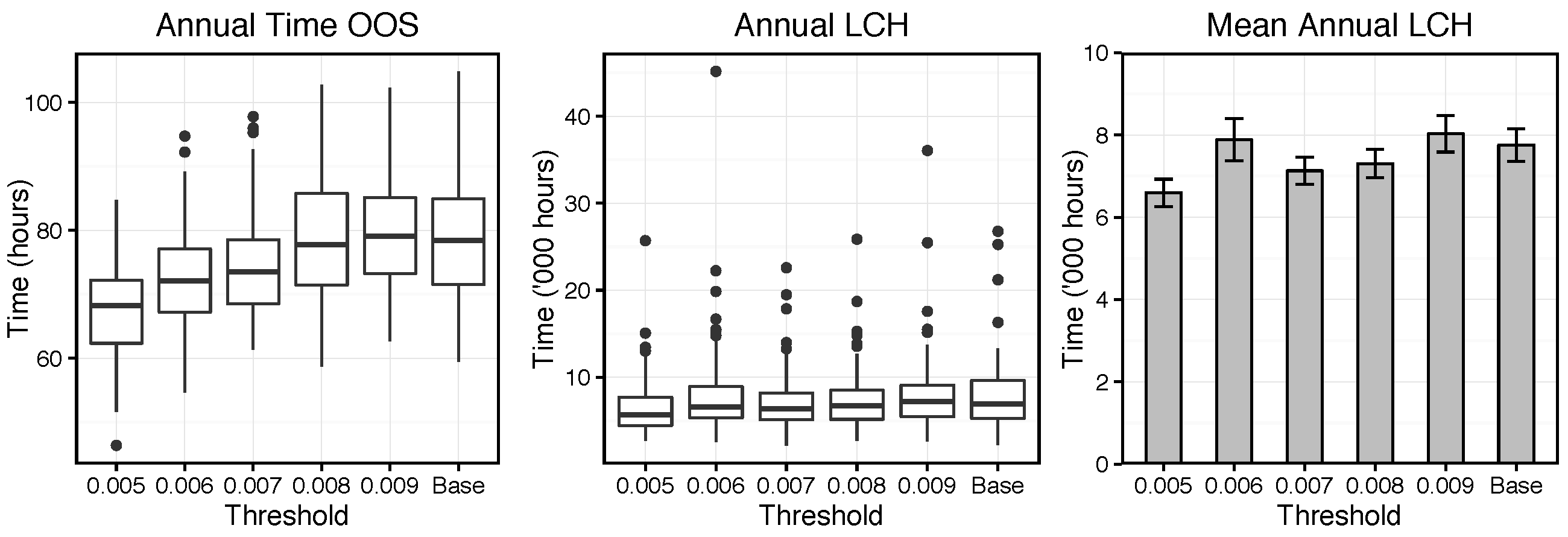
Figure 9 presents the output at each simulation setting. The left graph shows box plots of the annual time Lift agents have spent out of service (OOS). The centre box plot displays the annual Lost Customer Hours (LCH) value accrued by the User agents as a consequence of disruptions. The right bar chart presents the same LCH values summarised as means, to avoid scaling to outliers.
A number of observations can be made from the left plot. Firstly, there is significant variation in the time OOS between simulations at the same threshold setting. This is a consequence of the stochastic nature of the ABM; each simulation run is distinct as different values are drawn from probability distributions embedded in the model. Secondly, a general trend is observed of reducing time OOS as the threshold parameter is lowered. At the threshold values of 0.008 and 0.009 the plot shows little impact from the addition of predictive maintenance into the model. However, once the threshold is reduced below this level the response becomes more apparent. This is an intuitive concept, as a lower threshold value would imply more predictive maintenance tasks were scheduled and the installation of condition monitoring sensors has a greater effect.
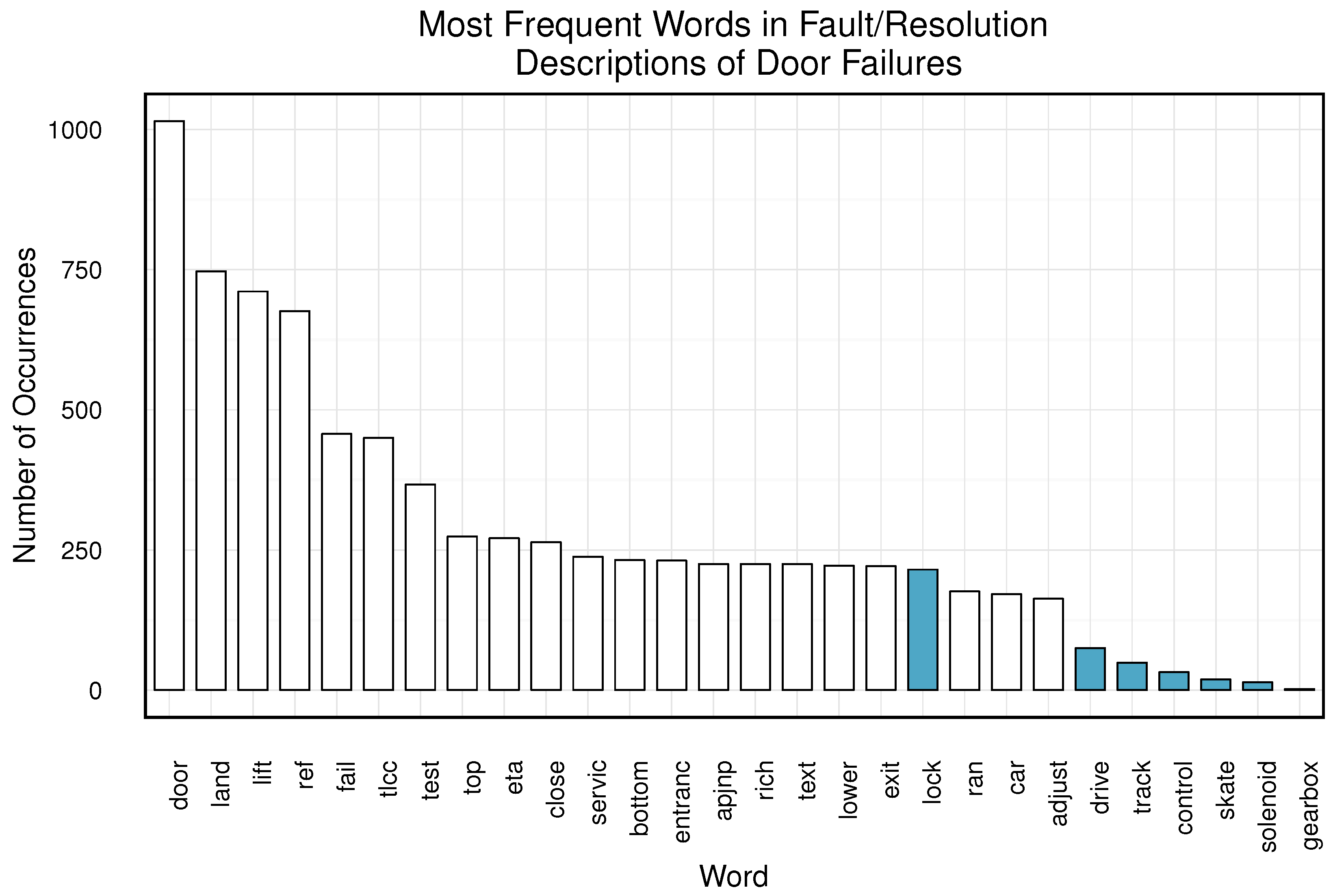
The magnitude of the reduction from the base case is perhaps not as significant as might be expected from the introduction of predictive maintenance capabilities. A potential cause for this rests in an assumption made in development of individual Component failure weightings: that they correspond to the Occurrence value from the FMEA document. This is not an unreasonable assumption as the FMEA analysis was completed by skilled engineers. However, exploratory frequency text mining of manually-typed Problem Description fields in the Failures Dataset provides opposing evidence to those values (see Appendix E). As the sensors are only assumed to monitor a subset of Components in a Lift, their impact is limited by these weightings.
The remaining plots in Figure 9 show the annual LCH for each threshold setting. The variation in these values is greater than for the previous output discussed and the box plot indicates a much larger number of outliers. The bar graph shows that the mean of the 0.006 threshold level is particularly affected by these anomalies. The reason for this large variation is believed to be a combination of the LCH calculation method, processes in the real system which the current model does not account for and the relatively short time period over which simulations were run.
As mentioned in the description of the User agent process, the LCH values calculated from these simulations use a literal interpretation of the term in absence of the method applied in the real system (see Equation (
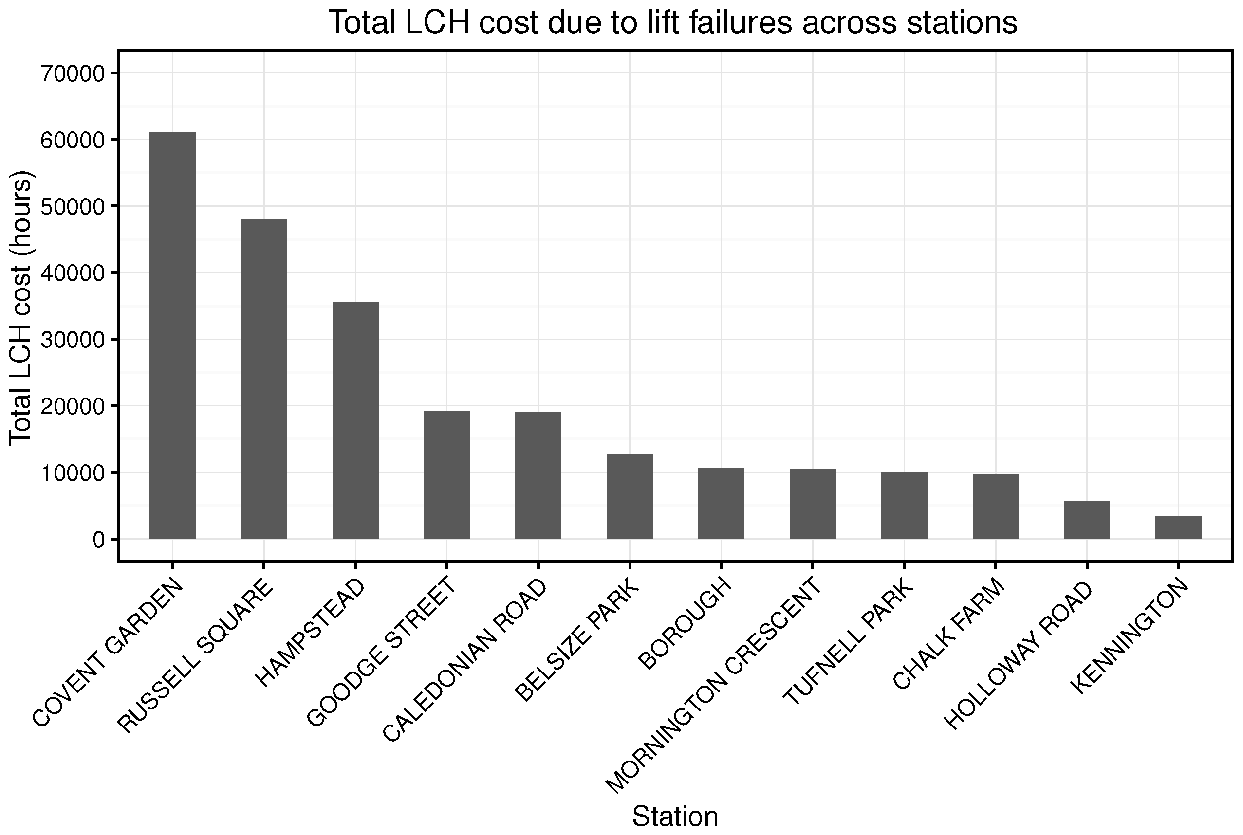
5)). Moreover, the model in its current form does not account for situations where a station can be closed as a result of asset failure. In the case of Covent Garden station, a single lift failing at a peak time of day (when over 1000 customers could be expected to travel through the station in either direction within a 15 min period) can force the station to shut. In these situations, the LCH value attributed to the event in the real system effectively has an upper bound.
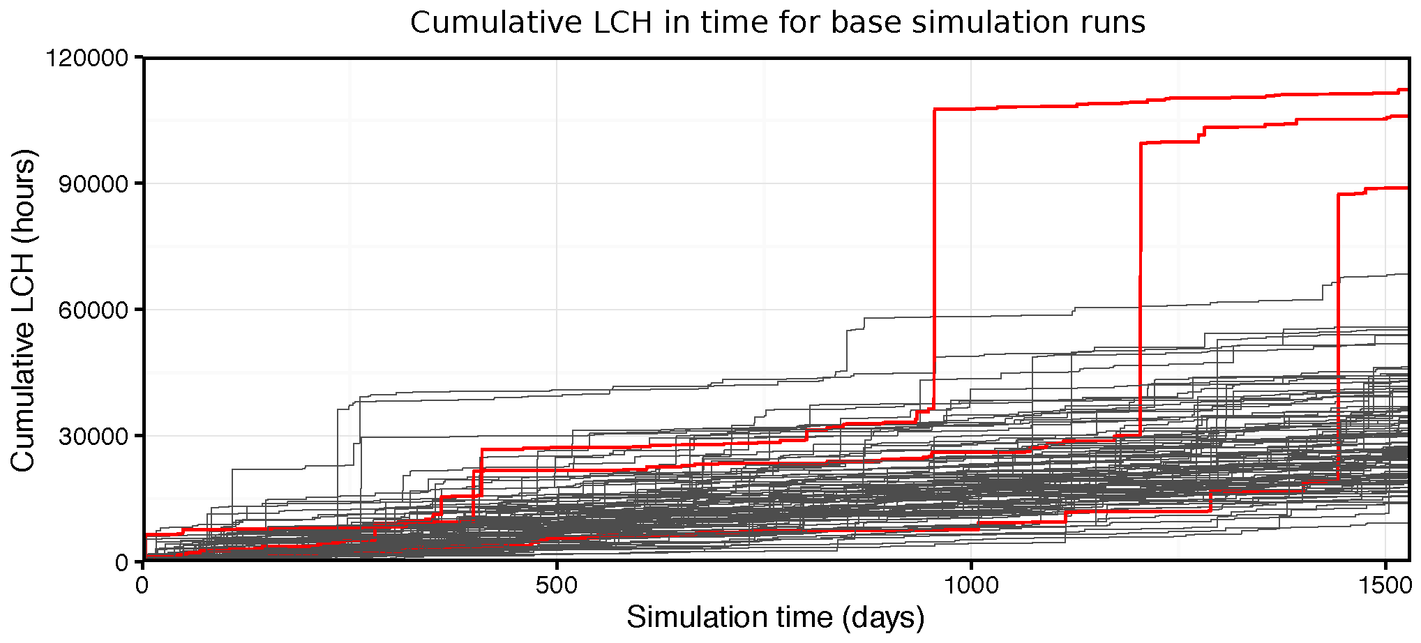
In contrast, if one of these rare events occurs within the simulation, it can have a significant impact on an individual run due to the lack of this upper bound. Figure 10 illustrates this effect. The plot shows the LCH accumulated over the course of multiple simulations (in this example the base case with no sensors) and three specific runs are highlighted in which these rare events arose. While the maximum waiting time of individual User agents was implemented to provide some stability in these circumstances, additional measures may be required to further take them into account.
Although a minor downward trend is observed in annual LCH with the introduction of sensors, it is difficult to assign a confident value in the face of this large variation. Nonetheless, this aspect of the results identifies a potentially useful, if unintended, application for the model in risk analysis (for example in estimating the likelihood of specific undesirable events occurring).

6.2. Return on Investment

It was possible to quantify the direct costs in the ABM results using the values discussed in Section 5.3. However, for the indirect costs, the LCH output obtained from the model was highly variable. Therefore, to characterise these indirect costs as a result of asset downtime in a more consistent way between simulations, a reference rate was inferred from the base model runs. The median of the LCH values from the base simulations was calculated and converted to an indirect cost per hour asset downtime (the median was used here as it is less affected by extreme outliers in the dataset and therefore an improved descriptor of the typical case in this situation). This reference value was subsequently applied in establishing indirect costs throughout the other simulations.
The average annual costs accrued during simulations were determined for each threshold setting. Initially, a very small set of values were observed to be having a significant impact on the mean costs. These were removed by setting limits at 2.5 absolute deviations around the median [122]. The annual saving rates were subsequently calculated by taking the difference between the annual costs for the base and predictive cases. Table 5 presents these results alongside mean multi-year RoI values. It is important to note there are large uncertainties introduced into these figures from the stochastic nature of the ABM, making it more challenging to draw conclusive insights.
As the threshold parameter is reduced, the results show that savings from predictive maintenance increase. These values also highlight a possible tipping point between thresholds of 0.007 and 0.008 . Above this value, there is no beneficial effect of predictive maintenance. This implies that monitored Components would generally fail before reaching the required threshold for the AssetManager to schedule predictive maintenance. Once this threshold is reduced, savings are achieved as additional predictive maintenance is performed in response to condition monitoring.
It may be expected an optimum should exist where the extra cost of predictive maintenance outweighs the realised benefits. However, the simulation results show no optimum value within the range of threshold levels investigated. A possible explanation for this could be additional complexities in the real system which the current model does not take into account.
These initial results were presented to experienced consultants within Amey Strategic Consulting and APJNP asset managers. Their feedback highlighted that at low values of the threshold level, the risk of false positive sensor readings could increase dramatically. In the real system, these type I errors can be introduced if minor deviations from an asset’s normal operating conditions breach a low failure threshold level despite there being no underlying problem. In these cases, if a decision is made based solely on whether asset conditions exceed this threshold, predictive maintenance could be carried out needlessly. This would incur extra cost without a corresponding benefit. Furthermore, this cost is not solely monetary. If a maintenance engineer is assigned to repair a part that is already in good condition, they may become sceptical of the true value of condition monitoring. These issues have the potential to undermine the effectiveness of the entire venture within an organisation.
Given the amount of predictive maintenance that occurs in the simulation at the lowest threshold in comparison to other levels, it was suggested that extra costs incurred as a result of the above considerations could significantly reduce or eliminate any benefit realised. The threshold settings at 0.006 and 0.007 were recommended to represent a more appropriate estimation of the RoI in this predictive maintenance strategy.
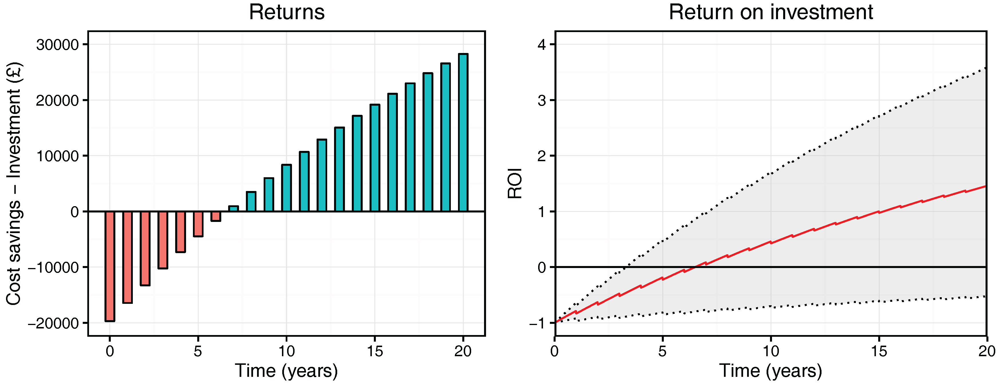
Figure 11 shows further detail of the estimated mean returns (Cost savings minus Investment) and discounted RoI for the threshold level of 0.006 . The grey shaded area in the RoI plot represents the range of outcomes as indicated from the variation in simulation results. A key aspect in both of these plots is the time taken to achieve a positive RoI. After this stage, the initial investment has been reclaimed and true returns start to be realised. The mean savings in both plots suggest this time would occur between 6 and 7 years after the initial installation (albeit with significant uncertainty).
The stochastic nature of the ABM also offers an insight into best- and worst-case scenarios. It is important to take these potential possibilities and risks into account when interpreting the results from the model. The right plot in Figure 11 shows that, in the worst-case, it could take a far greater period of time for a positive RoI to be realised. This is a consequence of lower savings and discounting applied to future values. Conversely, in the best-case scenario, the results suggest a positive RoI could be achieved approximately 3 years after sensor installation.
The question that this case study was initially developed to address was what is the RoI of installing remote condition monitoring sensors on lift doors in Covent Garden station? The current results suggest that a positive RoI can be realised in approximately 6 to 7 years, after which returns would continue to accrue and increase the RoI value. However, it is important to note the wide range of outcomes observed in the ABM output.
The results also imply that a positive RoI will only occur if an effective predictive maintenance strategy is implemented alongside the sensor installation. If readings from the sensors are disregarded and not acted upon (i.e., the threshold parameter is above the tipping point), the benefits of such a system may not be achieved. Similarly, if the data is not analysed appropriately and the derived information interpreted incorrectly by the asset manager (i.e., the threshold parameter is too low), extra costs can be incurred by unnecessary maintenance which could offset any potential benefit.

6.3. Suggestions for Future Work

The results produced by this ABM present an interesting view of the business case for installing condition monitoring sensors on lift assets. It would be desirable to use the insights gained up to this point to progress development of the model further, in keeping with the previously suggested data mining revision process [74,87]. Unfortunately, this was not possible within the scope of the current work. This section proposes questions which could be addressed in future research to realise a more complete approximation of the real system.

6.3.1. How Does the Failure Model Affect the Results?

The failure behaviour developed in this model only represents one of a number of ways to describe this aspect of the system. A more complex behaviour could be developed using one of the techniques discussed in Section 2.1.4, such as hidden Markov models or a form of Bayesian updating. A major limitation to the development of the former would be the lack of sufficient data regarding door lift failures, but this could be somewhat alleviated through a combination with the latter.
An advantage of redesigning the failure behaviour using the Bayesian updating approach would be that the sensors themselves could be more rigorously simulated. It was noted in the previous section that at lower threshold levels we could expect more false positive alerts, but the current ABM does not account for this. As Bayesian updating allows one to assign probability values to the sensor correctly identifying the asset’s condition state, the method would enable the ABM to capture this additional level of complexity.
A further factor to consider in the failure probability could be to build an interaction between the Behaviour object and the User agents. The theory behind this consideration is that the lifts may be more likely to undergo treatment that leads to failure when a large number of customers are passing through them, for example by trapped objects in doors. This heightened likelihood of failure could be characterised by temporarily increasing the failure probability of specific Components during busy periods throughout a day.
In addition, insight gathered from APJNP asset managers suggested that heterogeneity could be an important consideration in the nature of asset failures. Each lift in this ABM is assumed to follow the same general failure behaviour but a future extension could incorporate a variation of behaviours between separate assets.

6.3.2. How Is the RoI Affected If the Extra Predictive Maintenance Is Offset by Removal of Planned Maintenance?

This case study has focused on applying predictive maintenance in addition to an existing planned maintenance schedule. The results highlight the need for a changed approach to maintenance within the asset management organisation if a condition monitoring strategy is to be effective. The introduction of predictive maintenance led to savings in emergency maintenance costs. However, these were partly offset by the existing planned maintenance schedules which remain constant between scenarios.
It only became apparent after these results were analysed that it would be valuable to study how a reduction in the frequency of maintenance tasks within predefined schedules would affect the overall RoI of the venture. For example, this could potentially be implemented by skipping planned maintenance in the simulation if condition data observed by the AssetManager agent suggests failure is unlikely. A difficulty here would be that the sensors are assumed to only provide information relating to certain Component objects. Therefore, reducing the planned maintenance would be removing work on some Components without supplying an alternative. A further consideration is that some of the planned maintenance work is required to satisfy industry standards in the real system. Further investigation would need to be conducted into which specific tasks could potentially be excluded.

6.3.3. Will Agent Intelligence Improve the RoI Outcome?

The complexity of the current model could be further increased through the introduction of more advanced agent decision-making processes. For the AssetManager agent, it would be interesting to incorporate forecasting ability into the predictive maintenance scheduling. Rather than the basic case of a constant threshold level to initiate predictive maintenance, the AssetManager could be extended with the ability to observe trends in condition. Further interviews with asset managers could also be conducted to design a more realistic behaviour for this agent.
The queueing system for the User agents could also be enhanced. The current model only takes into account two choice preferences. Application of more advanced queueing theory may create interesting interactions between Users in different queues waiting for Lifts, which could have a consequential effect on their efficiency in passing through the station. For example, jockeying could be added where Users dynamically move between queues if they believe they may be able to board an earlier Lift.

6.3.4. How Does the ABM Scale in Time?

A number of assumptions had to be made when considering how the results evolved over long periods of time. The current failure behaviour is based on relatively recent historical data and so it may not continue to apply far into the future. Additionally, the complete refurbishment or replacement of lift assets is not accounted for in the ABM. Finally, the possibility of the sensor hardware itself failing and requiring replacement is not considered in the calculations. In extending the model, it would be valuable to assess how incorporating these longer-term aspects affects the value added by condition monitoring.

6.3.5. How Does the ABM Scale in Space?

This work only addresses the installation of sensors at a single, but critical, station on the London Underground. In future work, it would be valuable to investigate whether similar returns can be realised at other locations with different agent parameters. It could perhaps be expected that the sensor network would not offer a good investment at quieter stations, where the same indirect cost savings could not be achieved from reducing asset downtime. From a more ambitious perspective, the scope of the ABM could be increased dramatically by combining multiple station models to represent an entire network of lift assets.

6.3.6. Could We Set Threshold Values in Order to Optimise KPIs?

A key aspect that could be explored when running large scale simulations (i.e., covering all lift assets) of the presented work is regarding the effect of different threshold values for different lifts. The reasoning behind this is that not all assets are equally important to an organisation, even when the assets could be exactly the same. As pointed out in this report, lifts at Covent Garden have a much greater influence on KPIs such as LCH than any other lift in the network. This implies that it is possible to tolerate lift failure at stations with low number of passenger (high threshold values could be used) while it is unacceptable to have lift failures at key stations such as Covent Garden (requiring low threshold values). In fact, threshold values could become a function of not just space/location but also time among other variables (lift failures at Covent Garden are more damaging on Saturday afternoon than on weekdays).

7. Conclusions

This research has investigated the potential of integrating ABMS and data science to answer practical business questions within infrastructure asset management. A specific application was addressed in the installation of condition monitoring sensors to London Underground lift assets in Covent Garden station. The developed ABM was supported by analysis of historical data to present an authentic view of the real system. Key areas for future work were also outlined.
The results from the case study offer a number of conclusions. The ABM suggests that condition monitoring sensors on lift assets for predictive maintenance could realise a positive RoI approximately 6 to 7 years following the initial installation. However, difficulty was noted in obtaining a conclusive result as there was a significant range of achievable outcomes owing to the stochastic nature of the model. It was also determined that, to realise a positive RoI, the asset management firm must ensure that the predictive maintenance strategy is appropriately implemented and adopted within its current maintenance system.
A key objective of this research was to investigate opportunities for combining ABMS and data science in the field of infrastructure asset management. Based on insights from this work, it is clear that this integration possesses great capacity for capturing the complexity of the modern world when compared to other forms of simulation and analysis. However, it has yet to fully graduate from its origins in theoretical application to a refined process for answering practical business questions. The hope is that the current work has highlighted the underlying value in this approach and will serve to further this emerging paradigm.

Acknowledgments

The authors would like to thank Amey Strategic Consulting and Technology for their support and encouragement, in particular the management team: Charles Oldham, Tom Bedeman, Jon Jarritt and Ian Gordon. The authors would also like to thank APJNP personnel for their assistance and willingness to create innovative solutions to London Underground most pressing problems, in particular Ben Langham and Andy Derbyshire.

Author Contributions

C.H. wrote most of the report and performed simulations and analysis; S.G.H., R.M., A.K. and Y.L. assisted with expertise, data acquisition and analysis as well as simulation design; finally P.B. conceived and supervised the entire project.

Conflicts of Interest

The authors declare no conflict of interest.

Appendix A. Initial Failure Analysis

Before commencing the design of the structure and agents of the ABM, it was necessary to further examine the nature of lift failures on the London Underground. This allowed insight to be obtained on the type of sensors that could be potentially installed to realise the greatest value from their measurements. After initially cleaning the Failures Dataset it was possible to evaluate the total LCH costs due to different lift component failures. Figure A1 shows these results. Note that only the data gathered from January 1, 2012 contained the fields required to categorise the failures in this way and entries with missing failure labels were excluded. The results show that Landings and Doors failures account for a vast majority of asset problems for this case, causing over 30,000 LCH in this period.
Additionally, analysis was conducted into the most critical stations in terms of LCH costs. The same dataset as above was used for this analysis. Figure A2 presents the outcome. This plot shows that particular stations on the network have historically incurred higher LCH costs, with Covent Garden and Russell Square as the worst offenders.
Figure A1. Total incurred LCH costs from lift component failures across the Jubilee, Northern and Piccadilly lines. Data shown is from the period 1 January 2012 to 16 March 2016.
Systems 05 00004 g016
Figure A2. Total incurred LCH costs from lift failures across stations, showing highest values. Data shown is from the period 1 January 2012 to 16 March 2016.
Systems 05 00004 g017

Appendix B. Contractor Response and Repair Times

The Work Orders Dataset was used to determine probability distributions from which the Contractor response and repair times could be drawn. After cleaning, the data was filtered to include only failures classified as Landings and Doors. The subsequent analysis process is outlined below.
Firstly, a ResponseTime field was created for each entry to be the time difference in minutes between the CreateDate and FirstOnSite timestamps for each failure event. Similarly, a RepairTime field was generated as the difference between FirstOnSite and RTSDate (return to service) timestamps. To clean the data, erroneous entries due to incorrect input were excluded. This involved the removal of negative time values and manual investigation of extreme outliers.
For the ResponseTime variable, maximum-likelihood fitting was applied to approximate the data by a lognormal distribution. Figure B1 shows the histogram and fitted distribution. Figure B2 presents the corresponding Q-Q plot (a method for graphical comparison of a dataset with a theoretical distribution to assess the goodness of fit). A lognormal distribution was also fitted to the RepairTime variable and the corresponding plots are shown in Figure B3 and Figure B4. Table B1 gives the parameters and standard errors for both estimated lognormal distributions.
The logarithmised mean and standard deviation, denoted as μ and σ respectively, can be related to the non-logarithmised mean and standard deviation, denoted as m and v , by Equations (B1) and (B2). For the response time, m and v were determined as 47.3 and 27.7 min respectively. For the repair time, m and v were evaluated at 114.9 and 100.6 min.
μ = ln m 1 + v m 2
σ = ln 1 + v m 2
In both cases, the figures show that the lognormal distribution fits the data relatively well. The Q-Q plot of ResponseTime deviates slightly from the fitted distribution at the right, indicating that this data is light-tailed. This would be expected of a bounded dataset when compared to an unbounded distribution. Furthermore, it is interesting to note the steps in Figure B4 which are likely a result of manual data entries by maintenance engineers leading to duplicate repair times at round values. Despite these minor discrepancies, these fitted distributions are an appropriate approximation to the real case for the purposes of the simulation.
Table B1. Estimated parameter values of the lognormal fit for response and repair times with standard errors, all given to 3 significant figures.
Response TimeRepair Time
EstimateSEEstimateSE
Log mean 3.71 0.0169 4.46 0.0235
Log SD 0.543 0.0120 0.754 0.0166
Figure B1. Histogram of response time to emergency maintenance of lifts with a fitted lognormal distribution shown.
Systems 05 00004 g012
Figure B2. Q-Q plot of response time to emergency maintenance of lifts with lognormal line shown.
Systems 05 00004 g013
Figure B3. Histogram of repair time of emergency maintenance of lift doors with a fitted lognormal distribution shown.
Systems 05 00004 g014
Figure B4. Q-Q plot of repair time of emergency maintenance of lift doors with lognormal line shown.
Systems 05 00004 g015

Appendix C. Policies

In the absence of information on the specific planned maintenance schedules for different lifts, the Work Orders Dataset was analysed to identify the different schedules. Each lift asset in the dataset was plotted on a graph showing the total number of work orders against the percentage of Planned Maintenance (PM) work orders. Figure C1 displays the output of this process. The graph additionally has a colour scale denoting the proportion of Emergency Maintenance (EM) work orders for each individual asset.
Figure C1. Total number of work orders plotted against proportion of Planned Maintenance (PM) work orders for each lift asset. Colour scale represents proportion of Emergency Maintenance (EM) work orders for each asset.
Systems 05 00004 g018
There is clear banding present in the plot, as highlighted by the dashed lines. It appears that each of these bands corresponds to a maintenance schedule on the network. The various schedules include different types of PM work, each carried out at distinct regular intervals. The names of different PM tasks could be determined from description fields in the data. Covent Garden station resides in the uppermost band, which represents the most intensive PM schedule.
Once the type of planned policy was understood, the dataset was subsequently used to determine the time intervals between the different tasks. Table C1 shows the values obtained for the group containing Covent Garden station.
Table C1. Mean time intervals and standard errors for planned maintenance schedule denoted as Schedule 1 in Figure C1. All values given to 1 decimal place.
Maintenance NameTime Interval (Days)
MeanSDSE
Type A Service 27.4 4.2 0.2
Type B Service 57.2 6.4 0.5
Type C Service 58.5 8.0 0.6
Six Monthly Clean 187.4 29.0 5.1

Appendix D. Component Failure

In order to determine a probabilistic view of Component failure rate, the nonhomogeneous Poisson Process (NHPP) as discussed in Section 2.1.4 was used to characterise the nature of lift failures over time. The equations developed by Crow [31] were used to approximate the parameters of the NHPP. What follows is a brief description of these equations and the approximation process.
We assume an asset is observed from time t = S to t = T , and that N failures occur in the observed time. Additionally, let X i denote the time of each failure within the observed time for ( i = 1 , , N ) . The following equations can then be used to calculate maximum likelihood estimates for the shape, β ^ , and scale, λ ^ , parameters of the NHPP for the asset [31].
β ^ = N i = 1 N ln T X i
λ ^ = N T β
The maximum likelihood estimates were calculated using the Failures Dataset. Initially, data was filtered to include only door-related failures at Covent Garden station. Failures were regarded as door-related when the Problem field of the dataset included the word Door. A single asset (lift 1) was selected for the analysis as it possessed the greatest number of data points. Using the above equations, maximum likelihood estimates were calculated to be β = 1.53 and λ = 2.43 × 10 4 .
The compatibility of the probability model can be evaluated using the Cramér-von-Mises goodness-of-fit test. This test was adapted for the NHPP by Crow [31] and the full process is outlined in that work. The parametric Cramér-von-Mises statistic, C m 2 , was evaluated as 0.249 for the maximum likelihood estimates calculated above with the real failure data. This is below the corresponding critical value at the 1 % significance level for the number of data points that exist ([31] Table 2).

Appendix E. Text Mining Failure Descriptions

In order to assess the validity of the assumption that Component failure weightings correspond to Occurrence values from the FMEA analysis, manually typed fault description fields of the Failures Dataset were analysed using text mining. Common English words were ignored and derivations of the same word (e.g., plurals) combined in this process. The results, shown graphically in Figure E1, contrast quite dramatically to the FMEA document. Most strikingly, locks and skates were not considered to be the most frequent occurrence in the FMEA but are mentioned far more often that other parts in the Failures Dataset.
Figure E1. Specific word frequencies in fault descriptions of the Failures Dataset. Component words are highlighted. The results only show the highest frequency words and words relating to Components.
Systems 05 00004 g019

Appendix F. Initialisation Details

Table F1. Task details as part of the Policy assigned to all Lifts in the simulation.
TaskTime Interval (Days)
Type A Service27
Type B Service57
Type C Service59
Six Monthly Clean187
Table F2. Details of door Components of Lifts in the agent-based model.
Component NameFMEA Occurrence RatingFailure WeightingCondition from Sensor?
Safety edges8 0.190 Y
Drive controls7 0.167 N
Running tracks8 0.190 Y
Locks and skates5 0.119 Y
Gearbox5 0.119 N
Knuckle/solenoid4 0.095 N
Other5 0.119 N

Appendix G. User Agent Reference Journey Costs

The reference journey costs for assessing the impact of disruptions on a User agent’s journey time through the station were generated by running multiple simulation runs over a three day period with no Lift failures. During each run, in every fifteen minute time period the mean journey cost for a User was evaluated. Ten simulation runs were completed using this process. The results were then averaged to produce the reference dataset used during the simulation. Figure G1 illustrates the output of this process.
Figure G1. User reference journey costs with no lift failures. Each grey line represents one simulation run, the red line is the mean of the 10 simulation runs.
Systems 05 00004 g020

References

  1. ISO. ISO 55000: Asset Management—Overview, Principles and Terminology; ISO: Geneva, Switzerland, 2014. [Google Scholar]
  2. IAM (The Institute of Asset Management). An Anatomy for Asset Management; IAM: Bristol, UK, 2014. [Google Scholar]
  3. ISO. ISO 55001: Asset Management—Management Systems—Requirements; ISO: Geneva, Switzerland, 2014. [Google Scholar]
  4. ISO. ISO 55002: Asset Management—Guidelines for the Application of ISO 55001; ISO: Geneva, Switzerland, 2014. [Google Scholar]
  5. IBM Software. Harness the value of big data to build smarter infrastructures. 2013. Available online: http://www-01.ibm.com/common/ssi/cgi-bin/ssialias?infotype=SA&subtype=WH&htmlfid=TIW14160USEN (accessed on 14 February 2016).
  6. Atzori, L.; Iera, A.; Morabito, G. The Internet of Things: A survey. Comput. Netw. 2010, 54, 2787–2805. [Google Scholar] [CrossRef]
  7. Zanella, A.; Bui, N.; Castellani, A.; Vangelista, L.; Zorzi, M. Internet of Things for Smart Cities. IEEE Internet Things J. 2014, 1, 22–32. [Google Scholar] [CrossRef]
  8. Reed, D.A.; Gannon, D.B.; Larus, J.R. Imagining the Future: Thoughts on Computing. Computer 2012, 45, 25–30. [Google Scholar] [CrossRef]
  9. World Economic Forum. Industrial Internet of Things: Unleashing the Potential of Connected Products and Services. 2015. Available online: http://www3.weforum.org/docs/WEFUSA_IndustrialInternet_Report2015.pdf (accessed on 5 March 2016).
  10. Feibel, B.J. Investment Performance Measurement; John Wiley & Sons: Hoboken, NJ USA, 2003. [Google Scholar]
  11. Mobley, R.K. An Introduction to Predictive Maintenance; Butterworth-Heinemann: Woburn, MA, USA, 2002. [Google Scholar]
  12. Botchkarev, A.; Andru, P.; Chiong, R. A Return on Investment as a metric for evaluating information systems: Taxonomy and application. Interdiscip. J. Inf. Knowl. Manag. 2011, 6, 245–269. [Google Scholar]
  13. HM Treasury. The Green Book: Appraisal and Evaluation in Central Government. 2003. Available online: https://www.gov.uk/government/uploads/system/uploads/attachment_data/file/220541/green_book_complete.pdf (accessed on 1 May 2016). [Google Scholar]
  14. Fitz-Gibbon, C.T. Performance Indicators, 2nd ed.; Multilingual Matters: Clevedon, Philadelphia, PA, USA, 1990. [Google Scholar]
  15. Parmenter, D. Key Performance Indicators: Developing, Implementing, and Using Winning KPIs, 3rd ed.; John Wiley & Sons: Hoboken, NJ, USA, 2015. [Google Scholar]
  16. Minnaar, J.R.; Basson, W.; Vlok, P. Quantitative methods required for implementing PAS 55 or the ISO 55000 series for asset management. S. Afr. J. Ind. Eng. 2013, 24, 98–111. [Google Scholar] [CrossRef]
  17. Erhun, F.; Keskinocak, P. Game theory in business applications. In Management Science and Engineering; Stanford University: Stanford, CA, USA, 2003. [Google Scholar]
  18. Kelly, A. Decision Making Using Game Theory; Cambridge University Press (CUP): Cambridge, UK, 2003. [Google Scholar]
  19. Lindstädt, H.; Müller, J. Making Game Theory Work for Managers; McKinsey Quarterly: New York, NY, USA, 2010; pp. 1–9. [Google Scholar]
  20. Walravens, N.; Ballon, P. Platform Business Models for Smart Cities: From Control and Value to Governance and Public Value. IEEE Commun. Mag. 2013, 51, 72–79. [Google Scholar] [CrossRef]
  21. Dhillon, B. Engineering Maintenance: A Modern Approach; CRC Press: Boca Raton, FL, USA, 2002. [Google Scholar]
  22. Mobley, R.K. Maintenance Engineering Handbook; McGraw-Hill: New York, NY, USA, 2014. [Google Scholar]
  23. Tinga, T. Application of physical failure models to enable usage and load based maintenance. Reliab. Eng. Syst. Saf. 2010, 95, 1061–1075. [Google Scholar] [CrossRef]
  24. Akyildiz, I.F.; Su, W.; Sankarasubramaniam, Y.; Cayirci, E. Wireless sensor networks: A survey. Comput. Netw. 2002, 38, 393–422. [Google Scholar] [CrossRef]
  25. Hodge, V.J.; O’Keefe, S.; Weeks, M.; Moulds, A. Wireless Sensor Networks for Condition Monitoring in the Railway Industry: A Survey. IEEE Trans. Intell. Transp. Syst. 2015, 16, 1088–1106. [Google Scholar] [CrossRef]
  26. Dorling, K.; Messier, G.G.; Valentin, S.; Magierowski, S. Minimizing the Net Present Cost of Deploying and Operating Wireless Sensor Networks. IEEE Trans. Netw. Serv. Manag. 2015, 12, 511–525. [Google Scholar] [CrossRef]
  27. Davis, D.J. An Analysis of Some Failure Data. J. Am. Stat. Assoc. 1952, 47, 113–150. [Google Scholar] [CrossRef]
  28. Meeker, W.Q.; Escobar, L.A. Statistical Methods for Reliability Data; John Wiley & Sons: New York, NY, USA, 2014. [Google Scholar]
  29. Cohen, A.C. Maximum Likelihood Estimation in the Weibull Distribution Based On Complete and On Censored Samples. Technometrics 1965, 7, 579–588. [Google Scholar] [CrossRef]
  30. Yong, J. Condition-Based Hazard Ra te Estimation and Optimal Maintenance Scheduling for Electrical Transmission System. Ph.D. Thesis, Iowa State University, Ames, IA, USA, 2006. [Google Scholar]
  31. Crow, L.H. Evaluating the reliability of repairable systems. In Proceedings of the Annual Proceedings on Reliability and Maintainability Symposium, Los Angeles, CA, USA, 23–25 January 1990.
  32. Roberts, W.T.; Mann, L. Failure predictions in repairable multi-component systems. Int. J. Prod. Econ. 1993, 29, 103–110. [Google Scholar] [CrossRef]
  33. Tsokos, C.P.; Rao, A.N.V. Estimation of failure intensity for the Weibull process. Reliab. Eng. Syst. Saf. 1994, 45, 271–275. [Google Scholar] [CrossRef]
  34. Sim, S.H.; Endrenyi, J. A failure-repair model with minimal and major maintenance. IEEE Trans. Reliab. 1993, 42, 134–140. [Google Scholar] [CrossRef]
  35. Bunks, C.; McCarthy, D.; Al-Ani, T. Condition-Based Maintenance of Machines Using Hidden Markov Models. Mech. Syst. Signal Process. 2000, 14, 597–612. [Google Scholar] [CrossRef]
  36. Beck, J.L.; Au, S. Bayesian Updating of Structural Models and Reliability using Markov Chain Monte Carlo Simulation. J. Eng. Mech. 2002, 128, 380–391. [Google Scholar] [CrossRef]
  37. Zhang, R.; Mahadevan, S. Model uncertainty and Bayesian updating in reliability-based inspection. Struct. Saf. 2000, 22, 145–160. [Google Scholar] [CrossRef]
  38. North, M.J.; Macal, C.M. Managing Business Complexity; Oxford University Press (OUP): New York, NY, USA, 2007. [Google Scholar]
  39. Griffin, A.F.; Stanish, C. An agent-based model of prehistoric settlement patterns and political consolidation in the Lake Titicaca Basin of Peru and Bolivia. Struct. Dyn. 2007, 2. [Google Scholar]
  40. Charania, A.C.; Olds, J.R.; DePasquale, D. Sub-Orbital Space Tourism: Predictions of the Future Marketplace Using Agent-Based Modeling. In Proceedings of the 57th International Astronautical Congress (AIAA), Valencia, Spain, 2–6 October 2006.
  41. Robertson, D.A. The Strategy Hypercube: Exploring Strategy Space Using Agent-Based Models. In Multi-Agent-Based Simulation III; Springer: Berlin/Heidelberg, German, 2003; Volume 2927, pp. 182–192. [Google Scholar]
  42. Lattner, A.D.; Dallmeyer, J.; Timm, I.J. Learning Dynamic Adaptation Strategies in Agent-Based Traffic Simulation Experiments. In Multiagent System Technologies; Springer: Berlin/Heidelberg, German, 2011; Volume 6973, pp. 77–88. [Google Scholar]
  43. Axelrod, R.; Tesfatsion, L. Guide for Newcomers to Agent-Based Modeling in the Social Sciences. In Handbook of Computational Economics; Elsevier BV: Amsterdam, The Netherlands, 2006; pp. 1647–1659. [Google Scholar]
  44. Schelling, T.C. Micromotives and Macrobehavior; WW Norton & Company: New York, NY, USA, 2006. [Google Scholar]
  45. Hatna, E.; Benenson, I. The Schelling Model of Ethnic Residential Dynamics: Beyond the Integrated-Segregated Dichotomy of Patterns. J. Artif. Soc. Soc. Simul. 2012, 15, 6. [Google Scholar] [CrossRef]
  46. Holland, J.H. Hidden Order: How Adaptation Builds Complexity; Basic Books: New York, NY, USA, 1995. [Google Scholar]
  47. Bonabeau, E. Predicting the Unpredictable. Harv. Bus. Rev. 2002, 80, 109–116. [Google Scholar] [PubMed]
  48. Amin, M. Toward Secure and Resilient Interdependent Infrastructures. J. Infrastruct. Syst. 2002, 8, 67–75. [Google Scholar] [CrossRef]
  49. Rinaldi, S.M.; Peerenboom, J.P.; Kelly, T.K. Identifying, understanding, and analyzing critical infrastructure interdependencies. IEEE Control Syst. Mag. 2001, 21, 11–25. [Google Scholar] [CrossRef]
  50. Yerra, B.M.; Levinson, D.M. The emergence of hierarchy in transportation networks. Ann. Reg. Sci. 2005, 39, 541–553. [Google Scholar] [CrossRef]
  51. Samuelson, D.A.; Macal, C.M. Agent-based simulation comes of age. OR/MS Today. 2006. Available online: http://www.orms-today.org/orms-8-06/fragent.html (accessed on 3 February 2016).
  52. Sanford Bernhardt, K.L.; McNeil, S. Agent-Based Modeling: Approach for Improving Infrastructure Management. J. Infrastruct. Syst. 2008, 14, 253–261. [Google Scholar] [CrossRef]
  53. Osman, H. Agent-based simulation of urban infrastructure asset management activities. Autom. Constr. 2012, 28, 45–57. [Google Scholar] [CrossRef]
  54. Batouli, M.; Mostafavi, A. A hybrid simulation framework for integrated management of infrastructure networks. In Proceedings of the 2014 Winter Simulation Conference, Savannah, GA, USA, 7–10 December 2014; pp. 3319–3330.
  55. Macal, C.M.; North, M.J. Agent-based modeling and simulation. In Proceedings of the 2009 Winter Simulation Conference (WSC), Austin, TX, USA, 13–16 December 2009.
  56. Helbing, D.; Balietti, S. How to Do Agent-Based Simulations in the Future: From Modeling Social Mechanisms to Emergent Phenomena and Interactive Systems Design; Technical Report; Santa Fe Institute: Santa Fe, NM, USA, 2011. [Google Scholar]
  57. Bonabeau, E. Agent-based modeling: Methods and techniques for simulating human systems. Proc. Natl. Acad. Sci. USA 2002, 99, 7280–7287. [Google Scholar] [CrossRef] [PubMed]
  58. Bush, S.; Henning, T.; Ingham, J.; Raith, A. Agent-Based Modelling, a Quiet Revolution in Asset Management. In Proceedings of the IPWEA Conference NZ: Leading Tomorrow’s Infrastructure-Collaborate, Transform, Deliver, Auckland, New Zealand, 26–28 June 2014.
  59. Taber, C.S.; Timpone, R.J. Computational Modeling; SAGE Publications: Thousand Oaks, CA, USA, 1996. [Google Scholar]
  60. Heppenstall, A.; Malleson, N.; Crooks, A. ‘Space, the Final Frontier’: How Good are Agent-Based Models at Simulating Individuals and Space in Cities? Systems 2016, 4, 9. [Google Scholar] [CrossRef]
  61. Nikolic, I.; Dijkema, G.P.J. On the development of agent-based models for infrastructure evolution. Int. J. Crit. Infrastruct. 2010, 6, 148–167. [Google Scholar] [CrossRef]
  62. Sawyer, R.K. Artificial Societies: Multiagent Systems and the Micro-Macro Link in Sociological Theory. Sociol. Methods Res. 2003, 31, 325–363. [Google Scholar] [CrossRef]
  63. Helbing, D. Derivation of non-local macroscopic traffic equations and consistent traffic pressures from microscopic car-following models. Eur. Phys. J. B 2009, 69, 539–548. [Google Scholar] [CrossRef]
  64. Bell, W.P. Adaptive Interactive Expectations: Dynamically Modelling Profit Expectations. Ph.D. Thesis, University of Queensland, Brisbane, Australia, 2009. [Google Scholar]
  65. Deissenberg, C.; van der Hoog, S.; Dawid, H. EURACE: A massively parallel agent-based model of the European economy. Appl. Math. Comput. 2008, 204, 541–552. [Google Scholar] [CrossRef]
  66. Siebers, P.O.; Macal, C.M.; Garnett, J.; Buxton, D.; Pidd, M. Discrete-event simulation is dead, long live agent-based simulation! J. Simul. 2010, 4, 204–210. [Google Scholar] [CrossRef]
  67. Hamill, L. Agent-Based Modelling: The Next 15 Years. J. Artif. Soc. Soc. Simul. 2010, 13, 7. [Google Scholar] [CrossRef]
  68. Tobias, R.; Hofmann, C. Evaluation of free Java-libraries for social-scientific agent based simulation. J. Artif. Soc. Soc. Simul. 2004, 7. [Google Scholar]
  69. Nikolai, C.; Madey, G. Tools of the trade: A survey of various agent based modeling platforms. J. Artif. Soc. Soc. Simul. 2009, 12, 2. [Google Scholar]
  70. Lee, J.; Filatova, T.; Ligmann-Zielinska, A.; Hassani-Mahmooei, B.; Stonedahl, F.; Lorscheid, I.; Voinov, A.; Polhill, J.G.; Sun, Z.; Parker, D.C. The Complexities of Agent-Based Modeling Output Analysis. J. Artif. Soc. Soc. Simul. 2015, 18, 4. [Google Scholar] [CrossRef]
  71. Balci, O. Verification validation and accreditation of simulation models. In Proceedings of the 29th Conference on Winter Simulation (WSC ’97), Atlanta, GA, USA, 7–10 December 1997; pp. 135–141.
  72. Klügl, F. A validation methodology for agent-based simulations. In Proceedings of the 2008 ACM Symposium on Applied Computing (SAC ’08), Ceará, Brazil, 16–20 March 2008.
  73. Hastie, T.; Tibshirani, R.; Friedman, J. The Elements of Statistical Learning, 2nd ed.; Springer: New York, NY, USA, 2009. [Google Scholar]
  74. Remondino, M.; Correndo, G. MABS validation through repeated execution and data mining analisys. Int. J. Simul. Syst. Sci. Technol. 2006, 7, 10–21. [Google Scholar]
  75. Xing, P.; Lees, M.; Nan, H.; Viswanthatn, T.V. Validation of Agent-Based Simulation through Human Computation: An Example of Crowd Simulation. In Multi-Agent-Based Simulation XII; Springer: Berlin/Heidelberg, Germany, 2012; pp. 90–102. [Google Scholar]
  76. Manenti, L.; Manzoni, S.; Vizzari, G.; Ohtsuka, K.; Shimura, K. An Agent-Based Proxemic Model for Pedestrian and Group Dynamics: Motivations and First Experiments. In Multi-Agent-Based Simulation XII; Springer: Berlin/Heidelberg, Germany, 2012; pp. 74–89. [Google Scholar]
  77. Herd, B.; Miles, S.; McBurney, P.; Luck, M. Verification and Validation of Agent-Based Simulations Using Approximate Model Checking. In Lecture Notes in Computer Science; Springer: Berlin/Heidelberg, Germany, 2014; pp. 53–70. [Google Scholar]
  78. Konur, S.; Dixon, C.; Fisher, M. Formal Verification of Probabilistic Swarm Behaviours. In Lecture Notes in Computer Science; Springer: Berlin/Heidelberg, Germany, 2010; pp. 440–447. [Google Scholar]
  79. Borshchev, A.; Filippov, A. From System Dynamics and Discrete Event to Practical Agent Based Modeling: Reasons, Techniques, Tools. In Proceedings of the 22nd International Conference of the System Dynamics Society, Oxford, UK, 25–29 July 2004; Volume 22.
  80. Forrester, J.W. System dynamics, systems thinking, and soft OR. Syst. Dyn. Rev. 1994, 10, 245–256. [Google Scholar] [CrossRef]
  81. Schieritz, N.; Milling, P.M. Modeling the forest or modeling the trees. In Proceedings of the 21st International Conference of the System Dynamics Society, 20–24 July 2003; pp. 20–24.
  82. Fishman, G.S. Principles of Discrete Event Simulation; John Wiley & Sons: New York, NY, USA, 1978. [Google Scholar]
  83. Dhar, V. Data Science and Prediction. Commun. ACM 2013, 56, 64–73. [Google Scholar] [CrossRef]
  84. Batini, C.; Cappiello, C.; Francalanci, C.; Maurino, A. Methodologies for data quality assessment and improvement. ACM Comput. Surv. 2009, 41, 1–52. [Google Scholar] [CrossRef]
  85. Hazen, B.T.; Boone, C.A.; Ezell, J.D.; Jones-Farmer, L.A. Data quality for data science, predictive analytics, and big data in supply chain management: An introduction to the problem and suggestions for research and applications. Int. J. Prod. Econ. 2014, 154, 72–80. [Google Scholar] [CrossRef]
  86. Guess, F.G.; Redman, T.C. Data Quality (Poor Quality Data: The Fly in the Data Analytics Ointment). In International Encyclopedia of Statistical Science; Springer: Berlin/Heidelberg, Germany, 2011; pp. 345–346. [Google Scholar]
  87. Baqueiro, O.; Wang, Y.J.; McBurney, P.; Coenen, F. Integrating Data Mining and Agent Based Modeling and Simulation. In Advances in Data Mining. Applications and Theoretical Aspects; Springer: Berlin/Heidelberg, Germany, 2009; pp. 220–231. [Google Scholar]
  88. Sen, S.; Sekaran, M. Multiagent coordination with learning classifier systems. In Lecture Notes in Computer Science; Springer: Berlin/Heidelberg, Germany, 1996; pp. 218–233. [Google Scholar]
  89. Dogra, I.S.; Kobti, Z. Improving prediction accuracy in agent based modeling systems under dynamic environment. In Proceedings of the 2013 IEEE Congress on Evolutionary Computation, Cancun, Mexico, 20–23 June 2013.
  90. Zhang, H. Data-Driven Agent-based Modeling of Innovation Diffusion. In Proceedings of the 2015 International Conference on Autonomous Agents and Multiagent Systems, Istanbul, Turkey, 4–8 May 2015; pp. 2009–2010.
  91. Hassan, S.; Pavón, J.; Antunes, L.; Gilbert, N. Injecting Data into Agent-Based Simulation. In Simulating Interacting Agents and Social Phenomena; Springer: Berlin/Heidelberg, Germany, 2010; pp. 177–191. [Google Scholar]
  92. Remondino, M.; Correndo, G. Data mining applied to agent based simulation. In Proceedings of the 19th European Conference on Modelling and Simulation, Riga, Latvia, 1–4 June 2005.
  93. Denz, N. Process-Oriented Analysis and Validation of Multi-Agent-Based Simulations. Ph.D. Thesis, University of Hamburg, Hamburg, Germany, 2014. [Google Scholar]
  94. Grimm, V.; Revilla, E.; Berger, U.; Jeltsch, F.; Mooij, W.M.; Railsback, S.F. Pattern-Oriented Modeling of Agent-Based Complex Systems: Lessons from Ecology. Science 2005, 310, 987–991. [Google Scholar] [CrossRef] [PubMed]
  95. Kugu, E.; Altay, L.; Sahingoz, O.K. Using Agent Based Modeling and Simulation for Data Mining. In Neural Information Processing; Springer: Berlin/Heidelberg, Germany, 2012; pp. 258–265. [Google Scholar]
  96. Arroyo, J.; Hassan, S.; Gutiérrez, C.; Pavón, J. Re-thinking simulation: A methodological approach for the application of data mining in agent-based modelling. Comput. Math. Organ. Theory 2010, 16, 416–435. [Google Scholar] [CrossRef]
  97. Sibertin-Blanc, C.; Villa-Vialaneix, N. Data Analysis of Social Simulations Outputs-Interpreting the Dispersion of Variables. In Multi-Agent-Based Simulation XV; Springer: Berlin/Heidelberg, Germany, 2015; pp. 133–150. [Google Scholar]
  98. Bijak, J.; Hilton, J.; Silverman, E.; Cao, V.D. Reforging the Wedding Ring: Exploring a Semi-Artificial Model of Population for the United Kingdom with Gaussian Process Emulators. Demogr. Res. 2013, 29, 729–766. [Google Scholar] [CrossRef]
  99. Pruyt, E.; Cunningham, S.; Kwakkel, J.H.; De Bruijn, J.A. From data-poor to data-rich: System dynamics in the era of big data. In Proceedings of the 32nd International Conference of the System Dynamics Society, Delft, The Netherland, 20–24 July 2014.
  100. Pruyt, E. Integrating Systems Modelling and Data Science: The Joint Future of Simulation and ‘Big Data’ Science. Int. J. Syst. Dyn. Appl. 2016, 5, 1–16. [Google Scholar] [CrossRef]
  101. Bhamidipati, S.; van der Lei, T.; Herder, P. A layered approach to model interconnected infrastructure and its significance for asset management. Eur. J. Transp. Infrastruct. Res. 2016, 16, 254–272. [Google Scholar]
  102. Moore, C.; Tjioe, M.; Manzella, A.; Sanford Bernhardt, K.L.; McNeil, S. Asset management insights using agent models. In Proceedings of the 7th International Conference on Managing Pavement Assets, Calgary, AB, Canada, 23–28 June 2008.
  103. Zechman, E.M. Agent-Based Modeling to Simulate Contamination Events and Evaluate Threat Management Strategies in Water Distribution Systems. Risk Anal. 2011, 31, 758–772. [Google Scholar] [CrossRef] [PubMed]
  104. Chu, J.; Wang, C.; Chen, J.; Wang, H. Agent-Based Residential Water Use Behavior Simulation and Policy Implications: A Case-Study in Beijing City. Water Resour. Manag. 2009, 23, 3267–3295. [Google Scholar] [CrossRef]
  105. Taillandier, P.; Vo, D.; Amouroux, E.; Drogoul, A. GAMA: A Simulation Platform That Integrates Geographical Information Data, Agent-Based Modeling and Multi-scale Control. In Principles and Practice of Multi-Agent Systems; Springer: Berlin/Heidelberg, Germany, 2012; pp. 242–258. [Google Scholar]
  106. Du, J.; El-Gafy, M. Virtual Organizational Imitation for Construction Enterprises: Agent-Based Simulation Framework for Exploring Human and Organizational Implications in Construction Management. J. Comput. Civ. Eng. 2012, 26, 282–297. [Google Scholar] [CrossRef]
  107. Zhu, J.; Mostafavi, A. Integrated simulation approach for assessment of performance in construction projects: A system-of-systems framework. In Proceedings of the Winter Simulation Conference 2014, Savannah, GA, USA, 7–10 December 2014.
  108. Knoeri, C.; Nikolic, I.; Althaus, H.; Binder, C.R. Enhancing Recycling of Construction Materials: An Agent Based Model with Empirically Based Decision Parameters. J. Artif. Soc. Soc. Simul. 2014, 17, 10. [Google Scholar] [CrossRef]
  109. Thomsen, J.; Levitt, R.E.; Kunz, J.C.; Nass, C.I.; Fridsma, D.B. A trajectory for validating computational emulation models of organizations. Comput. Math. Organ. Theory 1999, 5, 385–401. [Google Scholar] [CrossRef]
  110. Remondino, M. Reactive and deliberative agents applied to simulation of socio-economical and biological systems. Int. J. Simul. 2005, 6, 11–25. [Google Scholar]
  111. Billari, F.; Fent, T.; Prskawetz, A.; Diaz, B.A. The “Wedding-Ring”: An agent-based marriage model based on social interaction. Demogr. Res. 2007, 17, 59–82. [Google Scholar] [CrossRef]
  112. MAX, Maximum uptime, all the time. Thyssenkrupp Elevator AG, 2016. Available online: https://max.thyssenkrupp-elevator.com/en/ (accessed on 14 July 2016).
  113. TfL Investment Programme Management Office. Business Case Development Manual (BCDM). 2008. Available online: https://www.whatdotheyknow.com/request/method_for_calculating_lch (accessed on 1 April 2016).
  114. Bünter, A. Elevator Installation Maintenance Monitoring Utilizing a Door Acceleration Sensor. U.S. Patent 8,678,143B2, 25 March 2014. [Google Scholar]
  115. Waspmote, Libelium. Available online: http://www.libelium.com/products/waspmote/ (accessed on 10 May 2016).
  116. MKR1000, Arduino. Available online: https://www.arduino.cc/en/Main/ArduinoMKR1000 (accessed on 10 May 2016).
  117. Wzzard, B-B Smart Worx. Available online: https://bb-smartsensing.com/wzzard-sensing-platform/ (accessed on 10 May 2016).
  118. Grimm, V.; Berger, U.; Bastiansen, F.; Eliassen, S.; Ginot, V.; Giske, J. A standard protocol for describing individual-based and agent-based models. Ecol. Model. 2006, 198, 115–126. [Google Scholar] [CrossRef]
  119. Grimm, V.; Berger, U.; DeAngelis, D.L.; Polhill, J.G.; Giske, J.; Railsback, S.F. The ODD protocol: A review and first update. Ecol. Model. 2010, 221, 2760–2768. [Google Scholar] [CrossRef]
  120. Bersini, H. UML for ABM. J. Artif. Soc. Soc. Simul. 2012, 15, 9. [Google Scholar] [CrossRef]
  121. An analytical railway. Railways Strategies. 2015, 117. Available online: http://www.railwaystrategies.co.uk/article-page.php?contentid=21969&issueid=644 (accessed on 20 June 2016).
  122. Leys, C.; Ley, C.; Klein, O.; Bernard, P.; Licata, L. Detecting outliers: Do not use standard deviation around the mean, use absolute deviation around the median. J. Exp. Soc. Psychol. 2013, 49, 764–766. [Google Scholar] [CrossRef]
Figure 1. Unified Modelling Language (UML) class diagram of entities in the agent-based model. Double side bars represent agents and single side bars represent objects. The colours correspond to the role of the entity in the simulation: blue represents people, yellow are part of the assets and green are included as an aspect of maintenance.
Systems 05 00004 g001
Figure 2. UML state diagram for the Lift agent during the simulation.
Systems 05 00004 g002
Figure 3. UML state diagram for the User agent during the simulation.
Systems 05 00004 g003
Figure 4. UML state diagram for the Contractor agent during the simulation.
Systems 05 00004 g004
Figure 5. Failure intensity and reliability functions in time of the approximated nonhomogeneous Poisson process.
Systems 05 00004 g005
Figure 6. Surface fitted to calibration simulation runs of the ABM. Parameters being varied are the effect of maintenance on failure probability. The output measured is the absolute difference in total lift time out of service in the time period 7 January 2012 to 7 January 2015 compared to the historical value. On the left plot, each red point represents the mean of five simulation runs.
Systems 05 00004 g006
Figure 7. Linear best-fit line for calibration of plannedEffect parameter showing difference in total lift time out of service between simulation runs and the real value from historical data. The shaded area shows 95% confidence intervals for the fitted line.
Systems 05 00004 g007
Figure 8. World Economic Forum industry survey [9].
Systems 05 00004 g008
Figure 9. Effect of threshold parameter on annual asset time out of service and Lost Customer Hours.
Systems 05 00004 g009
Figure 10. Cumulative Lost Customer Hours over time for 100 simulation runs at base settings (no sensors installed). So-called rare events are highlighted as sharp jumps in a few simulations leading to a dramatic effect in the final output.
Systems 05 00004 g010
Figure 11. Returns and discounted return on investment over time for threshold level of 0.006 . The range of possible outcomes is highlighted by the shaded area in the return on investment plot.
Systems 05 00004 g011
Table 1. Summary of related agent-based models.
Author(s)Application/Model ImplementationAgentsDefinition of Agent BehavioursModel Evaluation
Sanford Bernhardt et al. [52]Infrastructure management/NoneAssets, Users, Asset managers, RegulatorsUndefinedn/a
Moore et al. [102]Infrastructure management/Matlab & RePastAssets, Users, Asset managers, RegulatorsViewpoint of author(s), Empirical data & Mathematical modelsIllustrative example
Osman [53]Infrastructure management/AnyLogic & Excel VBAAssets, Users, Asset managers, RegulatorsViewpoint of author(s) & Case studiesCase study, Verification & Validation
Batouli et al. [54]Infrastructure management/AnyLogicAssets, Users, Asset managersViewpoint of author(s) & Mathematical degradation modelIllustrative example
Zechman [103]Infrastructure management/AnyLogic & EPANETUsers, Asset managersViewpoint of author(s) & Water distribution system modelCase study
Chu et al. [104]Infrastructure management/Swarm, Visual Basic & MatlabRegulators, Water appliance market, UsersViewpoint of author(s), Empirical data & Mathematical modelsCase study & Validation
Bhamidipati et al. [101]Infrastructure management/GAMA [105]Assets, Users, Asset managersViewpoint of author(s) & Mathematical modelsCase study
Du et al. [106]Construction management/Not statedStaff, Managers, PresidentViewpoint of author(s) & Case studiesCase study, Verification & Validation
Zhu et al. [107]Construction management/AnyLogicDesigners, Workers, Risk ManagersViewpoint of author(s)Illustrative example
Knoeri et al. [108]Construction management/NetLogoEmployees, Stakeholders, AuthoritiesEmpirical dataCase study & Validation
Remondino et al. [74]Biological/JASSpeciesViewpoint of author(s)Case study & Parameter tuning
Arroyo et al. [96]Population dynamics/RePastPopulationViewpoint of author(s) & Empirical dataCase study & Clustering techniques
Bijak et al. [98]Population dynamics/RePastPopulationViewpoint of author(s) & Empirical dataCase study & Statistical emulators
Table 2. Summary of data used in development of the ABM.
NameTimeframeRelevant Content
Failures Dataset27 June 2010–16 March 2016Failure events related to lifts and escalators across the APJNP network.
Work Orders Dataset1 January 2015–23 March 2016Details of work orders on lifts and escalators across the APJNP network. Includes both planned and emergency maintenance.
Lift Specificationsn/aTechnical specifications of lift assets managed by APJNP.
Failure Mode and Effect Analysis (FMEA)n/aLift system reliability study completed by APJNP engineers.
TfL Passenger Count DataOne week, November 2012Entry/exit counts to London Underground stations in 15-min intervals.
TfL Business Case Development Manual [113]n/aDetails of considerations for business cases in the London Underground.
Table 3. Overview of entities for the simulation model.
Entity NameAttribute NameAttribute TypeDescription
LifttraveldoubleVertical distance between floors (m)
speeddoubleAverage vertical speed (m/s)
capacityintStated maximum passengers
actualCapacity *doubleFactor accounting for real capacity
boardingTimedoubleTime for unload/load cycle at floor (s)
hasSensorbooleanIndicator for sensor installation
topQueue/bottomQueueList<User>Queues for this Lift
ridersList<User>Users on board this Lift
partsList<Component>Component objects of this Lift
UsertypeUserTypeDirection of travel ({Exiting, Entering})
targetLiftLiftCurrent lift choice
journeyTimedoubleRecorded time (min)
waitingTimeWeightdoubleWeighting factor for time in queues
onLiftTimeWeightdoubleWeighting factor for time on board Lift
valueOfTimedoubleFinancial value of time (£/min)
maxWaitTime *doubleLimit to waiting time (min)
ContractorresponseDelaydoubleTime to respond to emergency maintenance (min)
repairTimedoubleTime to repair Lift (min)
currentTaskTaskAssigned Task object
plannedEffect *doubleEffect of planned maintenance
emergencyEffect *doubleEffect of emergency maintenance
predictiveEffect *doubleEffect of predictive maintenance
AssetManagerthreshold *doubleMeasure of risk aversion
emListList<Task>List of emergency Tasks
pmListList<Task>List of planned/predictive Tasks
policiesList<Policy>List of all Policies
monitorPartsList<Component>Components monitored by sensors
ComponentfailProbdoubleCurrent instantaneous failure probability
failBehaviourBehaviourCharacterises failure probability in time
timeFromLastFaildoubleTime from previous Component failure (min)
failWeightingdoubleWeighting factor used to determine failure probability
parentComponentComponent above in hierarchical structure
childrenList<Component>Component(s) below in hierarchical structure
ownerLiftLiftLift under which Component lies
BehaviourbetadoubleShape NHPP parameter
lambdadoubleScale NHPP parameter
TasktypeTaskTypeMaintenance type ({Planned,Emergency,Predictive})
targetLiftLiftLift corresponding to this maintenance
createTimedoubleTime of Task creation (min since sim start)
firstOnSiteTimedoubleTime of Contractor arrival (min since sim start)
finishTimedoubleTime of Task completion (min since sim start)
PolicytaskListList<Task>List of planned maintenance Tasks
liftListList<Lift>Lifts for this maintenance schedule
repeatIntervalsList<double>Repeating time schedule for Tasks (days)
Starred (*) attributes were not derived from analysis of historical data, as the required data does not exist or could not be obtained. Other attributes are either parameters based on analysis of historical datasets or aspects of model operation.
Table 4. Parameter values for entities in the simulation.
EntityAttributeValueUnitsSource
Lifttravel 35.3 mLift Specifications
speed 1.5 m/sLift Specifications
capacity50UsersLift Specifications
actualCapacity N ( μ = 0.8 , σ = 0.1 ) n/aEstimate from observation
boardingTime40sBCDM [113] (Appx D1)
partssee Appendix Fn/aFMEA
UserwaitingTimeWeight 2.5 n/aBCDM [113] (Table E3a)
onLiftTimeWeight 2.0 n/aBCDM [113] (Table E3a)
valueOfTime 10.15 £/hourBCDM [113] (Table E1a)
maxWaitTime10minEstimate
ContractorresponseDelay ln N ( μ = 3.71 , σ = 0.54 ) minWork Orders Dataset
repairTime ln N ( μ = 4.46 , σ = 0.75 ) minWork Orders Dataset
plannedEffect 0.7 n/aCalibration
emergencyEffect 1.0 n/aCalibration
predictiveEffect1.0n/aEqual to emergencyEffect
AssetManagerpoliciessee Appendix Fn/aWork Orders Dataset
ComponentfailWeightingsee Appendix Fn/aFMEA
Behaviourbeta (shape) 1.53 n/aFailures Dataset
lambda (scale) 2.43 × 10 4 n/aFailures Dataset
PolicytaskListsee Appendix Fn/aWork Orders Dataset
repeatIntervalssee Appendix Fn/aWork Orders Dataset
Table 5. Summary of annual saving rates for each threshold value and multi-year returns on investment for those resulting in a net saving.
ThresholdSavings Rate from Simulations (£/Year)Sensor Running Costs (£/Year)Mean 5-Year RoI (%)Mean 10-Year RoI (%)Mean 20-Year RoI (%)
0.005 5600 ± 2700 −1000898239
0.006 4300 ± 2900 −1000−2342143
0.007 3900 ± 2900 −1000−3225114
0.008 ( 2100 ± 3200 ) −1000---
0.009 ( 3700 ± 3100 ) −1000---

