1. Introduction
Being able to predict the health of a stockpile or population of units with confidence is beneficial for planning and for greater understanding about drivers of change in reliability. Reliability is an important aspect of the performance of complex systems. It is defined as the probability that the item will perform as intended in a specified environment for a specified duration and task. If stockpile managers are able to understand what causes changes in reliability, then management and handling of the stockpile can potentially be adapted to extend the service lifetime of some of the units. Prognostics and Health Management [
1] seeks to leverage improved understanding about influences on reliability to improve management strategies. In military applications, two types of management errors are possible: (1) taking a unit out of service prematurely can waste resources, as a useable unit is scrapped and replaced with another often costly unit; (2) leaving an unreliable unit in the field too long can risk having it fail in a critical situation, causing a safety or mission problem. Often, a unit will be chosen for use based upon a false impression that a newer unit will provide better performance. This leaves older units in the stockpile, where they continue to age and degrade, instead of placing priority on utilizing those items which are projected to go bad first to both remove low reliability items from the stockpile before crossing a reliability threshold and maintain mission readiness. In other settings, there are often similar tradeoffs between prematurely abandoning the unit from use and attempting to use it too long. Greater understanding of what causes changes in the reliability of the units can allow for more precise management strategies, and fewer costly errors. In addition, with more automated management systems for inventory and the cheaper availability of smaller sensors, it may be possible to gather unit-by-unit histories of handling, environmental exposure and usage. This information allows more detailed understanding of what the units have experienced, and more accurate predictions of reliability at the unit or lot (a small sub-population of the overall population grouped by manufacturing run) level. The building block for this improved modeling hinges on the availability of high quality data and a method to connect handling, exposure and usage to changes in reliability.
Reliability engineers often seek to describe the relationship between these inputs through a scientific or engineering-based first principles model. Developing these models can be expensive and labor-intensive, and there are still problems in connecting the understanding gleaned from them to the actual experiences of the units in the stockpile. Moreover, these investigations are limited to what is expected to degrade or cause degradation, and unknown degradation mechanisms are unaccounted for. For example, a laboratory experiment may show that there is a relationship between temperature cycling and a particular failure mode, but how this translates into different observed reliabilities for units in the stockpile that have each experienced a slightly different temperature exposure is difficult to make precise; this can be compounded by an acceleration factor utilized in a lab environment to represent more extended exposure.
In this paper, we describe a process that takes readily available data on individual units and uses this information to potentially improve the quality of reliability predictions, as well as provide a quantitative ranking of the ability of different models to explain patterns in reliability seen in the data. Note: in the remainder of this paper, the term “model” means “statistical model”. The process is flexible to handle different types of explanatory data as well as a variety of types of reliability data, including: (a) pass/fail data observed at different ages of the system; (b) degradation data measured on a continuous scale with a known or estimated threshold for when the unit will fail; (c) lifetime data if the unit is observed until it fails or is censored; and (d) destructive test results from representative members of a lot. The modeling can be performed on reliability data for individual failure modes or at the overall system level.
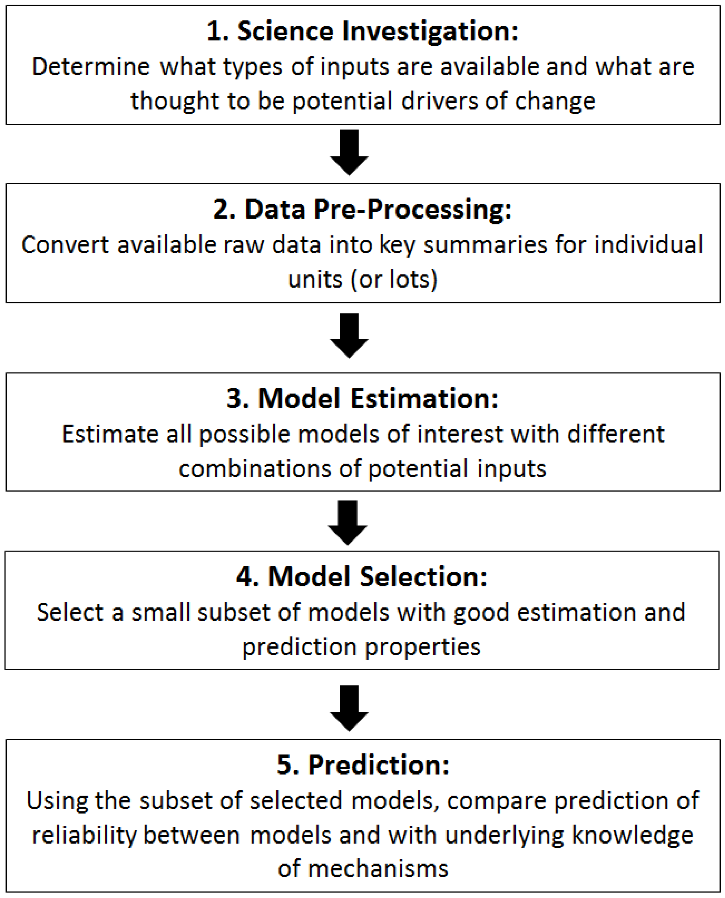
Figure 1 shows a flowchart of the process for evaluating the contributions of different potential explanatory variables summarizing the history of individual units on reliability. Ideally, in the first step “Science Investigation”, there would be scientific or engineering understanding that would drive the choices of which potential explanatory variables to consider in the models for reliability. For some failure mechanisms temperature cycling might be more important than absolute temperature, while for other mechanisms humidity might be of paramount importance. In most applications, the age of the unit is considered a potentially important influencer of reliability; other common choices for potential explanatory variables affecting reliability include: temperature, humidity, shock, vibration, manufacturer, usage and handling. Obtaining the list of explanatory variables that will be considered is the first step in determining what models can be examined and compared and is critical to completing the process with meaningful results.
Figure 1.
Flowchart of process for investigating the relationship between potential inputs and reliability.
Figure 1.
Flowchart of process for investigating the relationship between potential inputs and reliability.
The second step, “Data Pre-Processing”, takes the raw data available for each unit and translates it into useable summaries. For example, a sensor may measure temperature hourly across the lifetime of the unit. To make this information useable in a model we create summaries such as average, minimum and maximum temperature; average amplitude of daily temperature cycling; or a binning of exposure hours by temperature bands. Since many summaries are possible from this raw data, leveraging any available scientific understanding of the mechanisms driving changes in reliability can make this part of the process more effective and cut down on having too many unrelated summaries. However, in the absence of first-principles understanding, a collection of typical summaries can still be helpful for highlighting empirical relationships that improve prediction over just age alone, while suggesting areas for further first principles investigation.
The third step, “Model Estimation”, fits a potentially large number of models with different subsets of the explanatory factors to describe changes in reliability. The form of the model changes for different summaries of reliability. For example, if the response is a condition-based continuous summary, a standard multivariate linear regression model [
2] of the form
can be used, where
is the condition-based measure for the
jth unit, and
is the
ith explanatory variable value for the
jth unit. The error term,
, is assumed to be Normally distributed with mean 0 and constant variance. The parameters of the model which are estimated from the data are
. If the response is pass/fail observed at a particular age and set of environmental conditions, then a generalized linear model (GLM), such as a logistic regression model may be appropriate. The form of this model is as follows:
For more details on GLMs, see Myers
et al. [
3], Dobson and Barnett [
4] and McCullagh and Nelder [
5].
To assemble the set of possible models to be considered, different combinations of the inputs can be used. In its simplest form, if there are k different inputs to be evaluated, then there may be 2k models, where each factor can independently be included or omitted. Some combinations of inputs may not make sense or may not exist during the exposure lifetime of the unit, and then these models can be pruned from the set to be considered.
The fourth step, “Model Selection”, evaluates the different models based on their ability to explain patterns in the data. There are multiple possibilities for criterion to evaluate the quality of fit of the models, including AIC (Akaike Information Criterion) [
6], BIC (Bayesian Information Criterion [
7], DIC (Deviance Information Criterion) [
8], the Median Posterior Model [
9] and Prediction-Based criteria [
10,
11]. One or more of these metrics can be selected to provide a ranking of the goodness of the models, depending on how the user plans to use them. Different Information Criteria emphasize a different balance between parsimony and good prediction, so finding a good match to the objectives of the study is important. The statistics literature has considered multiple possible criteria for model selection. Many of these metrics are closely related, we encourage selecting a metric that mirrors study goals and how the final model will be used by the practitioners. In addition, cross-validation can be used to show the robustness of results for different subsets of the data and to provide assurance that the identified leading models perform well. Typical goals include estimation of model parameters to provide information about the nature of the relationship between the inputs and reliability, and/or prediction of reliability for a particular combination of inputs. In particular, there is frequently interest in extrapolating in order to predict the reliability of the system for ages in the future. As a result of this stage, the large collection of potential statistical models can be pruned to a smaller set with the best performance, as measured by the selected metric(s).
The fifth and final step, “Prediction”, examines what patterns of reliability are predicted using the top models identified in the previous step. Graphical summaries of the relationship between the inputs and reliability are produced to illustrate what impact different values of the inputs have on the expected reliability. Subject matter expertise combined with cost and quality considerations are all considered to select the top one or two models that best match current understanding of the underlying science and engineering and will be used for estimation and prediction in the future. Once the final models are identified, then Analysis of Variance (ANOVA) can be used to formally check for the significance of different terms in the model, and adequacy of the model assumptions, such as normality and the error term having constant variance, can be assessed.
The process and its possible results are illustrated in the next section using an example.
3. Reliability Data
In this Section, we examine the data using simple summaries and graphical methods to gain some initial understanding of its characteristics before proceeding with a formal assessment of the contributions of different input factors for predicting reliability. As part of the data pre-processing step, this exploratory data analysis (EDA) can help identify potential problems with the data, which can help us interpret the results and determine which models are best when we perform the formal analysis and model selection. For this case study, the reliability data consist of 1200 observations, with 973 “Pass” and 227 “Fail”, giving a simple
reliability estimate. For this data, there were no missing values. If some of the information about different units is incomplete, then a strategy for handling missing data should be considered. First, if there is no available information on the “Pass/Fail” status of the units, then these should be removed from the data considered in the analysis. Second, if some of the explanatory variables are missing data, then there are several choices about how to proceed:
Remove the unit with the missing values from consideration—this will reduce the overall size of the dataset, but will make comparisons between different models fair and consistent.
Remove the variable with the missing values from consideration—this maintains the size of the dataset, but does not allow investigation of different models with that as an explanatory variable. However, this strategy may be a good choice if a large proportion of the data is missing a particular variable, since future data may also suffer from this, and selecting a best model where information for that variable will not be available can be problematic.
Impute the missing values—this strategy allows missing values to be constructed based on available information from the rest of the data [
13], but is dependent on the assumption that the missing values are not systematically missing for a specific reason.
Table 1,
Table 2,
Table 3 and
Table 4 show some summaries of the distribution of units and their associated simple estimates of reliability for the example. In
Table 1, we see that there are more observations for younger systems, with less data in the windows between 40–50 and 50–60 months. This is connected to the fact that manufacturers 3, 4 and 5 have only been producing units for a shorter range of time, and hence there are no data to evaluate these units after a given age (52 months for manufacturer 3, and 38 months for manufacturers 4 and 5). In addition, we have included the binned reliability for each 10 month range. The overall trend in reliability is as expected, with older units being less reliable.
Table 1.
Summary information based on age.
Table 1.
Summary information based on age.
| Age | [0,10) | [10,20) | [20,30) | [30,40) | [40,50) | [50,60] |
|---|
| # obs | 215 | 256 | 244 | 222 | 132 | 131 |
| X/n | 87.4% | 85.9% | 81.1% | 80.6% | 72.0% | 71.0% |
Table 2.
Summary information based on manufacturer.
Table 2.
Summary information based on manufacturer.
| Manufacturer | 1 | 2 | MG = 1 | 3 | 4 | 5 | MG = 2 |
|---|
| # obs | 425 | 289 | 714 | 188 | 119 | 179 | 486 |
| X/n | 75.5% | 82.4% | 78.3% | 86.2% | 86.6% | 83.2% | 85.2% |
Table 3.
Summary information based on exposure.
Table 3.
Summary information based on exposure.
| Exposure | A | B | C | D |
|---|
| # obs | 379 | 562 | 201 | 58 |
| X/n | 92.9% | 75.8% | 70.1% | 93.1% |
Table 4.
Summary information based on version or damage.
Table 4.
Summary information based on version or damage.
| Version | a | b | c | Damage | 0 | 1 |
|---|
| # obs | 539 | 449 | 212 | # obs | 1118 | 82 |
| X/n | 81.1% | 80.4% | 82.5% | X/n | 81.2% | 79.3% |
Table 2 shows similar information when we partition the 1200 observations based on the different manufacturers. Manufacturer 1 has the largest proportion of the data, with the lowest estimated reliability. However, since there are differences in the ages of the units within each of the subpopulations, and there are more older units from manufacturers 1 and 2, we should be cautious about over-interpreting these results. Recall that the subject matter experts felt that manufacturers 1 and 2 are more similar to each other than to manufacturers 3, 4 and 5. Hence two different ways of partitioning the data by manufacturer or by manufacturer group (MG) are considered. The number of observations and the simple estimated reliability for each collection of units is provided.
Table 3 and
Table 4 show matching summaries based on partitioning the 1200 units by the four categories of exposures (
Table 3), the three categories of Version (left side of
Table 4) or by Damage, where “0” means that no superficial damage was observed on the unit. There are relatively few observations for exposure “D”, and only a small fraction of the units (82/1200 = 6.8%) has any recorded evidence of superficial damage.
We now highlight a number of areas of potential concern which are helpful to check before proceeding with subsequent model fitting and evaluation. While not extreme in this example, it is important to examine if one or more category within a factor does not have much observed data. For example, since there is such a small fraction of observed units with damage, there may not be sufficient information to adequately assess whether there are differences between the two categories of the damage factor. If one or more category has very little data, then it may be helpful to use expert opinion to try to determine if that data can be combined with another category based on understanding of the units.
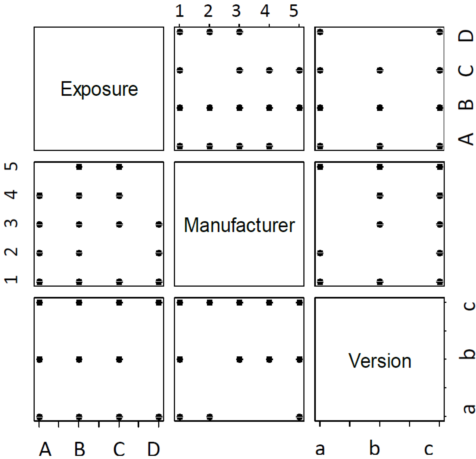
Figure 2 shows pairwise plots of exposure (E), manufacturer (M) and version (V), where a black dot indicates that there is at least one observation with a combination of attributes, and blank space indicates no data for that combination. For example, in the pairwise plot for exposure and manufacturer, we see that there are no data available for the following combinations: (E,M) = (A,5), (C,2), (D,4), (D,5). Similarly, there are missing combinations for (E,V) = (D,b), and (M,V) = (2,b), (3,a), (4,a). This is helpful to note, since when we try to make predictions based on some of these combinations of factors, they will be based on leveraging patterns across the entire dataset, instead of based on observations for that combination.
Figure 2.
Pairwise plot of all represented combinations of input factors observed in data.
Figure 2.
Pairwise plot of all represented combinations of input factors observed in data.
If two or more of the variables are measuring similar information, then the assessment of the models with these combinations of variables may be compromised because of the inability to distinguish which variables are contributing to changes in the observed reliability.
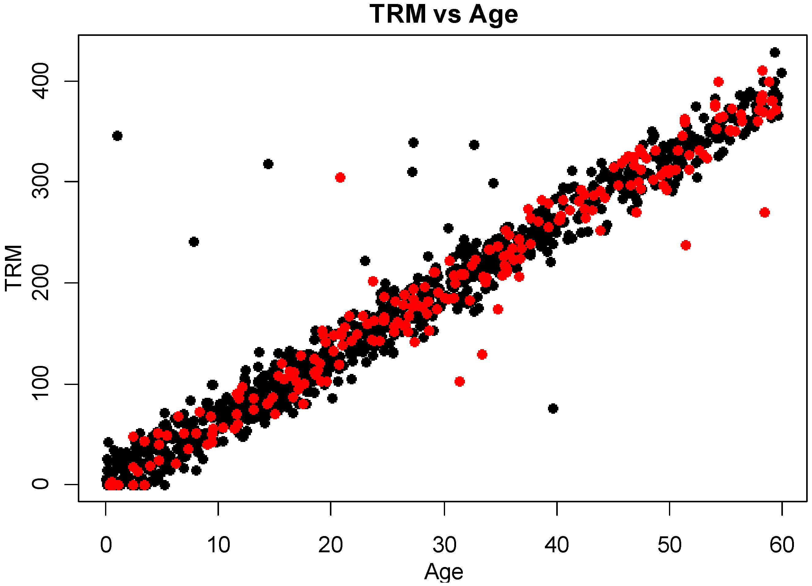
Figure 3 shows a scatterplot of time in ready mode (TRM—the usage measure for the units in our case study) and age. Black circles indicate an observed “Pass”, while red indicates a “Fail”. The calculated correlation between these two variables is 0.975, indicating that knowing the age of a particular system provides quite specific information about what range of TRM might be expected. There are a few observations which do not follow the strong trend between these two measurements, but overall there may be little additional information gained by including both age and TRM. When formal modeling is performed with both factors, the user should be cautious about interpreting the estimated coefficients since unstable estimated model parameters with large uncertainty is a known problem with multicollearity [
12]. A common solution to resolving problems with multicollinearity is to restrict estimation to models with just one of the problematic sets of variables. We return to this as a solution from our model selection after various models have been considered.
Figure 3.
Scatterplot of time in ready mode versus age, with tests resulting in a “Pass” shown in black, and those resulting in a “Fail” shown in red.
Figure 3.
Scatterplot of time in ready mode versus age, with tests resulting in a “Pass” shown in black, and those resulting in a “Fail” shown in red.
Finally, we note that several of the variables under consideration for models are continuous (age and TRM), while others are categorical in nature. When we choose to include a continuous variable in the model, it can be added with a single term (and a single degree of freedom) if we wish to examine the main effect or linear contribution of that factor on the response. If we wish to allow greater flexibility with the model, additional terms can be added to the model (say a quadratic or cubic term). When we include categorical variables in our model, then the number of degrees of freedom required to include that variable will typically be k−1, where k is the number of categories observed. Some variables could be included as either continuous or categorical. For example, consider that we have data available on the year of manufacturer. The year could be added as a continuous factor using a single degree of freedom: this would allow examining a linear trend across the years. An alternative would be to have separate categories for each year. This does not imply any connection between adjacent years, but rather allows each year to have a potentially different and unrelated effect on reliability compared to other years. If such a variable is included in the dataset, then it may be helpful to consider models that treat it as continuous and categorical separately, to determine which approach seems to yield better results. However, it would not make sense to consider models that include both of these choices simultaneously. In addition to selecting how the variables will be included in the model, there are also options about whether to include interactions between the variables. Because of the flexibility of the method that allows the user to specify any models that they wish to consider, we recommend that a combination of main effect only models and models including interactions be examined.
In the next section we consider what models to evaluate for estimating the reliability of the stockpile. Some of the features of the case study data that were identified in this exploratory analysis phase of the analysis will become important when we assess the performance of different models.
4. Modeling and Analysis
Recall that the goal of selecting a best model is to achieve good prediction of future reliability for individual units, with the ability to distinguish different subpopulations, and to leverage current engineering understanding of the reliability mechanisms. We also want a relatively uncomplicated model. One of the advantages of the model selection approach of this paper is that it is easy to consider a relatively large number of alternatives and quickly obtain a ranking for which candidate models look the most promising based on our identified priorities.
For the case study, we have available data for age (A), exposure (E), manufacturer (M), version (V), damage (D) and time in ready mode (TRM, or just T). We wish to consider all possible sensible models based on different combinations of these variables. For all of the variables except manufacturer, there are two options for the statistical model: include or exclude the variable. For manufacturer, we have three choices: exclude it, include it as summarized by the five levels of manufacturer directly (M), or include it using the two groups (MG, abbreviated as G). The inclusion or exclusion of a variable in the model can be determined independently for each of the variables. This leads to 96 possible models (2(A) × 2(E) × 3(M/G) × 2(V) × 2(D) × 2(T)). We use the naming convention that if a model includes a variable, then its label will include that letter. Omitted variables are not included in the label. For example, AEG is a model that includes age, exposure and manufacturer group (G). The largest possible model is AEMVDT, while the smallest model (denoted with “•”) is the null model with only the intercept. An enumerated list of all the models organized into a standardized structure is as follows:
•, A, E, AE, M, AM, EM, EAM, G, AG, EG, EAG,
(all 12 combinations of A, E and either M or G)
V, AV, EV, AEV, MV, AMV, EMV, EAMV, GV, AGV, EGV, EAGV,
(same combos with V added)
D, AD, ED, AED, MD, AMD, EMD, EAMD, GD, AGD, EGD, EAGD,
(same combos with D added)
VD, AVD, EVD, AEVD, MVD, AMVD, EMVD, EAMVD, GVD, AGVD, EGVD, EAGVD,
(same combos with both V and D added)
Repeat the above 48 model all with T included. Note the first line of the next set of models is
T, AT, ET, AET, MT, AMT, EMT, EAMT, GT, AGT, EGT, EAGT.
The advantage of the above structure is that it makes building a list of all of the models straightforward and intuitive. As the number of variables considered grows, it is helpful to use some structure to help with the efficient enumeration of all possible candidate models. If, for another example, some models do not make sense to consider, then they can be removed from the list.
An additional set of models can be specified if interactions between factors are considered. Including interaction terms in the model makes the predicted fits for different combinations of factors more flexible. For example, for a model with age and exposure with no interactions, we assume that the effect of age is the same for all levels of exposure, but just with a potential shift in the intercept in Equation (2). The same model including an interaction term allows for different shapes of reliability curves for different exposures. For this example, we consider only two-way interactions and make the additional assumption that it makes sense to include interactions if the two main effects are included in the model. In design of experiments, this principle is commonly called factor hierarchy, and is assumed in many statistical models, since the interpretability of results is greatly aided by this assumption. Since there are many possible models with two-way interactions when there are multiple variables included, we make the additional assumption and consider only those models where all two way interactions are included. For example, if we have a model AE, then there is only one two-way interaction that can be included (between age and exposure). If we have a model with AED, then our model would include all three two-way interactions age-exposure, age-damage and exposure damage.
With the inclusion of interactions (with the hierarchical assumption and including all two-way interactions for all pairs of variables in the model), this adds an additional 88 models. From the list of 96 models listed above, only those models with 0 (•) or 1 (A, E, M, G, V, D, T) variable are not included. We use the naming convention of adding an “i” after a model name to indicate that it includes the two-way interactions. For example AEDi would be the model with age, exposure, damage and the three possible two-way interaction terms.
We note that there is considerable flexibility in identifying the models to evaluate. For a moderate number of input factors, it is possible to consider all of the sensible combinations for combining the terms. It is straightforward to automate the identification of all models if there are no restrictions on which factors can be combined. Since estimating the parameters for each model is not time-consuming, a potentially large set of models can be considered. In other applications, we have evaluated over a thousand models with the goal of identifying the top few to examine in more detail. If the number of inputs leads to an unmanageably large number of choices then the practitioner can limit the choices to more promising candidates or look at groups of potential inputs sequentially in manageable groups to identify more promising contributors. We encourage the user to not be too nervous about looking at a larger number of models, since in our experience we have found that there are sometimes important surprises about which factors are beneficial that were not consider leading candidates a priori.
With the models to be evaluated now enumerated, we use statistical software to estimate all of the models and evaluate them with the chosen criterion. For this case study, the user selected the corrected AIC (Akaike Information Criterion) [
6], which is a common choice for model evaluation and managing the bias-variance tradeoff [
14], (p. 37). The form of the criterion, which is evaluated for each of the fitted models, is
with the first term, also called the deviance in the statistics literature, measuring how well the model can explain the patterns in the data by quantifying the amount left unexplained, and the second term is a penalty for complexity, since given equal predictive power, a simpler model is preferred. The corrected AIC makes a correction for finite sample sizes, with the formula
where n is the sample size (1200 for our example) and p is the number of model parameters.
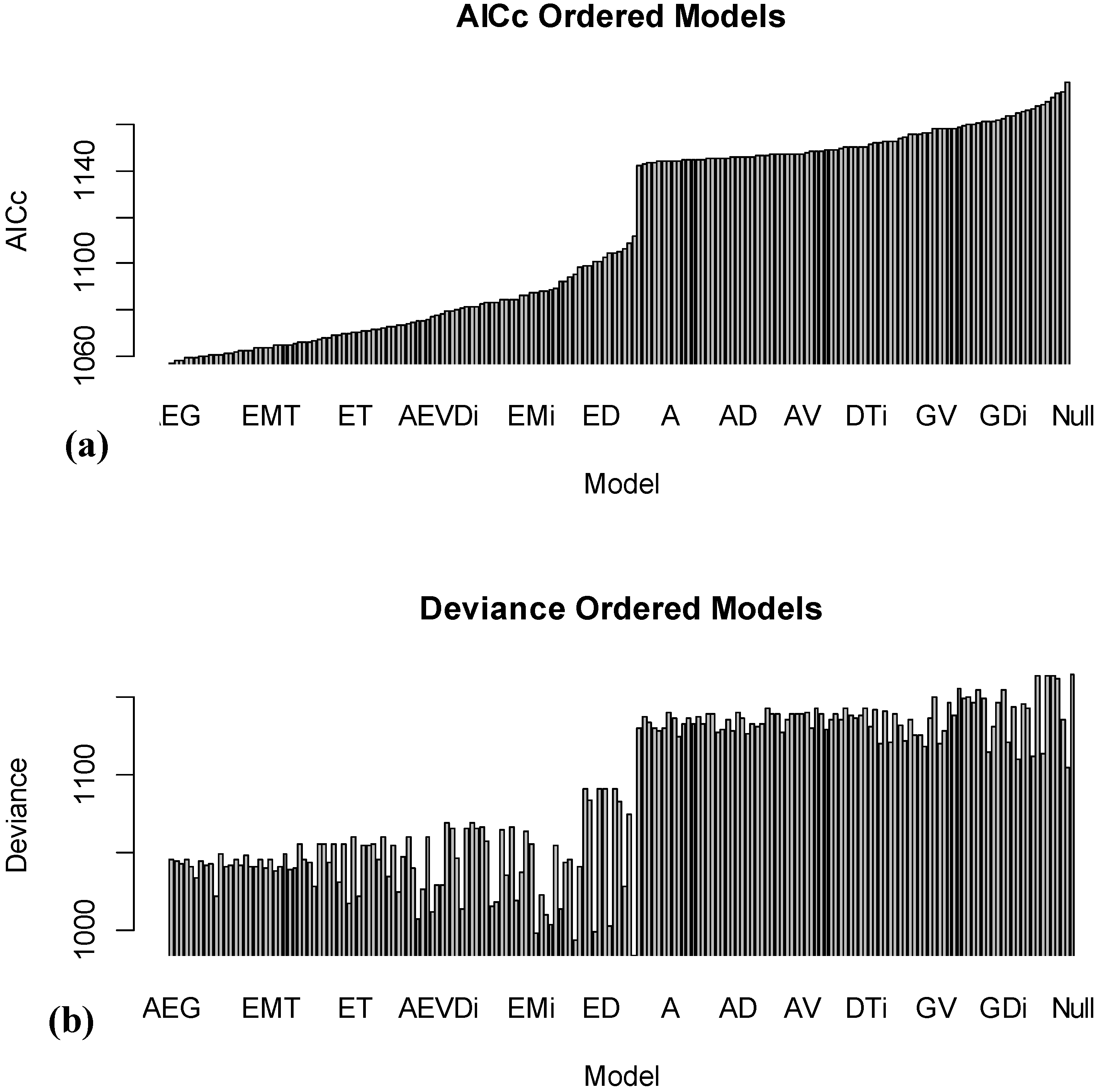
Figure 4a shows the sorted AICc values for fitting all 184 (96 models with no interactions, and 88 models with interactions). The best model is AEG, with several other models achieving similar performance.
Figure 4.
Results of fitting 184 models using different combinations of age (A), exposure (E), manufacturer (M), manufacturer group (G), version (V), damage (D) and TRM (T), including two-way interactions.
Figure 4.
Results of fitting 184 models using different combinations of age (A), exposure (E), manufacturer (M), manufacturer group (G), version (V), damage (D) and TRM (T), including two-way interactions.
The approach of fitting many models and looking at relative scores is advantageous since we can examine which of the top models actually makes the most sense given our current understanding of the drivers of change in reliability. While the AICc values in
Figure 4a show the overall trend in sorted models from best to worst,
Table 5 shows the top 20 models as ranked by the AICc criterion. By considering the degrees of freedom (DF) and the deviance columns, it is possible to gain a deeper understanding of competing top models. For example, the second best model, AEGT, leaves slightly less unexplained with a deviance of 1043.95 (
versus 1044.94 for the AEG model), but at the cost of a slightly more complex model (using 6 DF instead of 5 DF for the AEG model).
Figure 4b shows the model deviances in the same order as the top (with AICc) values. As can be seen, there are a number of models (near the left middle of the plot) with smaller deviances, implying that they are able to explain more of the patterns in the observed data. However, this highlights the advantage of using the AICc criterion, since it balances model complexity with the ability to explain patterns. These models are not that highly ranked with AICc because they require a very large number of model parameters to describe the patterns, and this overfitting [
14] of the model, which chases idiosyncrasies of the data instead of bigger trends, typically does not lead to good results when we wish to predict reliability for new data.
Table 5.
Summary information based on version or damage.
Table 5.
Summary information based on version or damage.
| | Model | AICc | DF | Deviance |
|---|
| 1 | AEG | 1056.99 | 5 | 1044.94 |
| 2 | AEGT | 1058.02 | 6 | 1043.95 |
| 3 | AEGV | 1058.18 | 7 | 1042.09 |
| 4 | AEGD | 1058.94 | 6 | 1044.87 |
| 5 | AEGVT | 1059.24 | 8 | 1041.11 |
| 6 | AEGi | 1059.25 | 12 | 1032.99 |
| 7 | AEGDT | 1059.99 | 7 | 1043.9 |
| 8 | AEGVD | 1060.09 | 8 | 1041.97 |
| 9 | AEM | 1060.23 | 8 | 1042.11 |
| 10 | AEGDi | 1060.5 | 18 | 1021.92 |
| 11 | EGT | 1060.52 | 5 | 1048.47 |
| 12 | AEGVDT | 1061.17 | 9 | 1041.01 |
| 13 | AEMT | 1061.32 | 9 | 1041.17 |
| 14 | EGVT | 1061.55 | 7 | 1045.46 |
| 15 | AEMV | 1062.18 | 9 | 1042.03 |
| 16 | EGDT | 1062.46 | 6 | 1048.39 |
| 17 | AEMD | 1062.55 | 10 | 1040.36 |
| 18 | AEMVT | 1063.29 | 10 | 1041.11 |
| 19 | EGVDT | 1063.45 | 8 | 1045.33 |
| 20 | AEMDT | 1063.65 | 11 | 1039.43 |
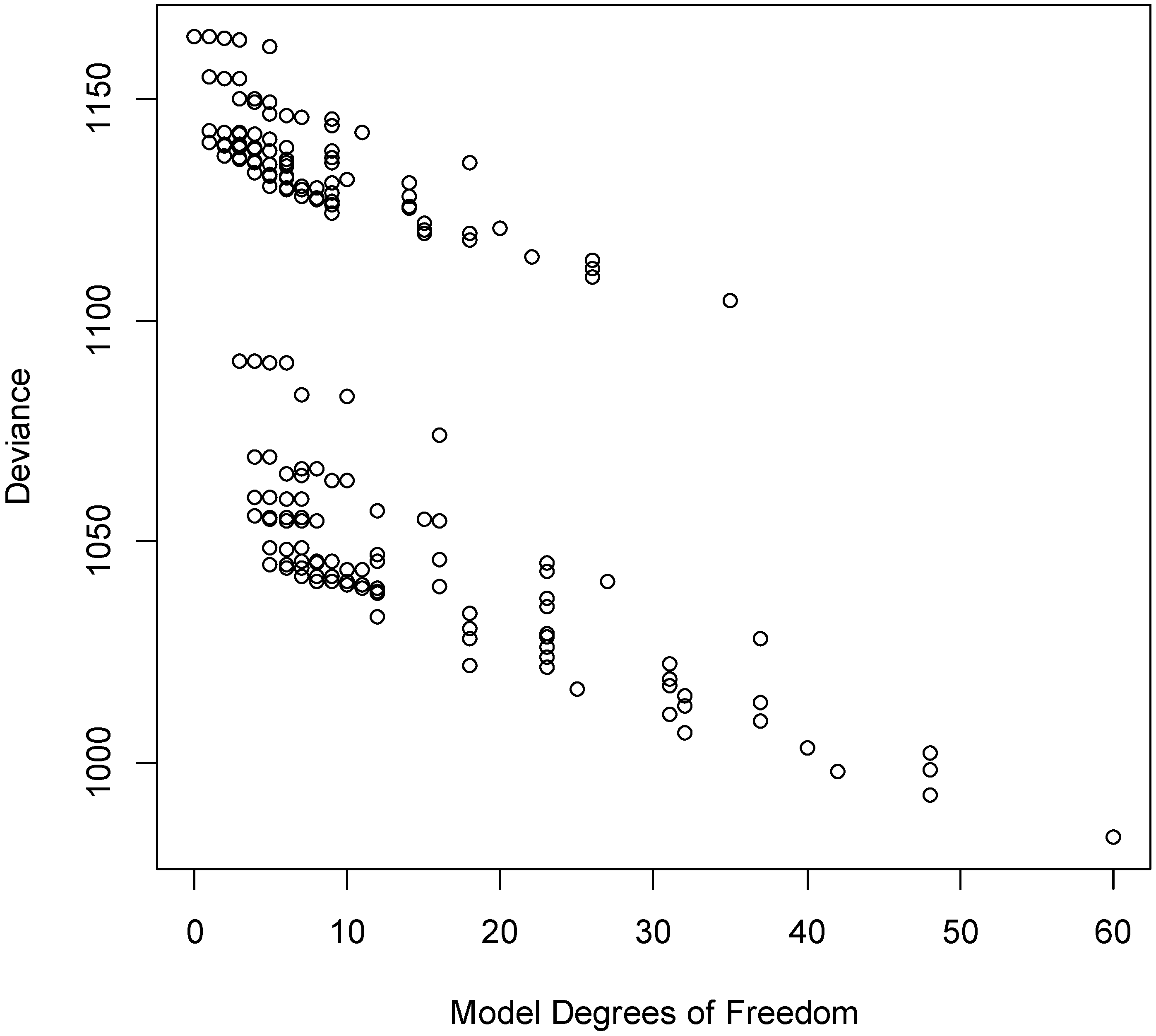
Figure 5 shows the general pattern of deviance
versus DF. Since this plot shows the two components of AICc directly, we can get a sense of the tradeoffs between the contributions. The Pareto front [
15,
16,
17] is the set of potential best values, depending on how we weight model complexity
versus deviance. It is the set of models which lie along the bottom left edge of the set of all models. For models on the Pareto front, the deviance can be reduced by making the model more complex, but these improvements are small relative to how much more complicated the model needs to become. In addition, there are large numbers of models (not on the Pareto front) with non-competitive deviance values, and these should typically be discarded from further consideration.
Traditionally, model selection algorithms have identified just a single best model. This approach considers the top models and compares them with current understanding of drivers of change in reliability from subject matter expertise to determine a best overall model. In addition, some models may be more expensive to collect the necessary data for future observations. If there is minimal marginal improvement with the addition of a potentially costly variable, the user may opt to use a simpler model with comparable performance. In the next section, we examine several of the top models, as identified by AICc, and examine the predictions across range of inputs of the included variables.
Figure 5.
Deviance versus degrees of freedom for 184 fitted models.
Figure 5.
Deviance versus degrees of freedom for 184 fitted models.
5. Results and Discussion
A final determination of a best model is made by balancing the empirical performance of the model from the model selection criterion (AICc here) with subject matter expertise of how well this matches current understanding. Based on the top 20 results in
Table 5, we note a few patterns:
All but two of the top 20 models include age. This suggests that there is a notable trend in reliability that can be modeled effectively with the inclusion of age. This matches current understanding of a key driver of change in reliability for the system.
Many of the top models include AEG, with the top eight models all including this combination plus other potential terms. This suggests that in addition to age, exposure and manufacturer group are effective ways of summarizing observed patterns. The simpler representation of manufacturer with the two groups (manufacturers 1 and 2 combined, and 3, 4 and 5 combined) is generally preferred to the more complex use of manufacturer directly.
The top five models all have quite similar deviance values, with the majority of the difference in their ranking being attributed to the complexity of the model with its associated penalty from the AIC criterion.
The 6th best model, AEGi, is the top model with a considerably smaller deviance value, but because of the three two-way interactions that have been included, it uses more degrees of freedom to achieve this improved fit.
Cross-validation was performed to evaluate the performance of the top 20 models. For each of 500 iterations, 20% of the data (240 observations) were removed from the data set, and the models were fit to the remaining 80% of the data. The estimated models were used to predict the responses for the 240 observations, and the quality of the fit was assessed. There was little change in the ranking of the top 10 models across the repeated resampling of the withheld data. Hence, the rankings based on the AICc appear robust to variations in the observed data used to fit the models.
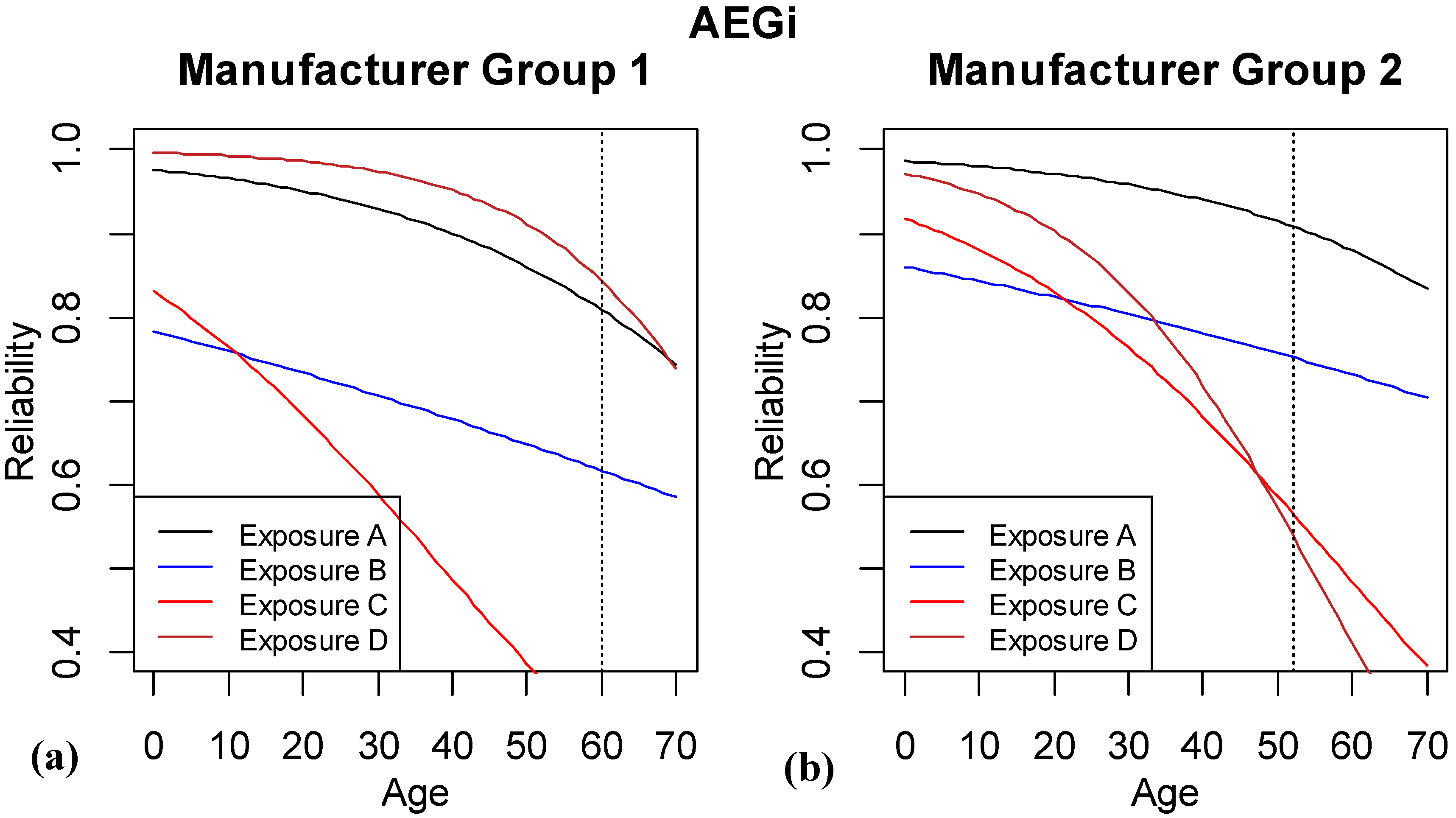
Based on this information, the engineers want to examine the predicted reliability for several models to see the patterns identified and compare it to available understanding. The models to be examined further are the top four models: 1. AEG, 2. AEGT, 3. AEGV, 4. AEGD, and the sixth best model AEGi, because of its smaller deviance value.
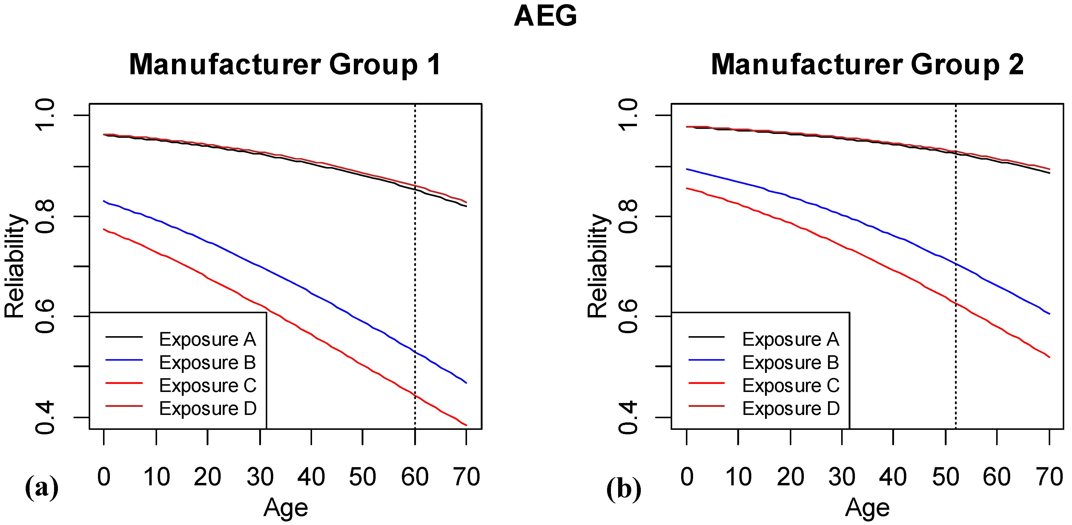
Figure 6 shows the eight lines that summarize the predicted reliabilities for the different factor combinations of the AEG model. There are four different exposure groups and two manufacturer groups. The reliability is shown for ages 0 to 70 months, where vertical dashed lines show the end of the observed data. For manufacturer group 1, the oldest tested system was approximately 60 months old, while for the second manufacturer group, the oldest system is near 52 months. To the right of the vertical lines, we are extrapolating to ages not yet tested. From examining differences between the lines, we can see that Exposures A and D are most similar and have the highest reliability, and manufacturer group 2 has better predicted reliability for any given age. The observed patterns (decreasing reliability with aging) and ordering of categories within a factor all match current understanding of the underlying mechanisms.
Figure 6.
Results of logistic regression model based on including age, exposure and manufacturer group. The vertical dashed line highlights where the last of the observed data are available.
Figure 6.
Results of logistic regression model based on including age, exposure and manufacturer group. The vertical dashed line highlights where the last of the observed data are available.
An alternative to modeling reliability directly might be to plot the predicted value of right hand side of Equation (2) versus the explanatory variables. This quantity is known as the “fitted log odds” and is a linear function of the explanatory variables that mirrors the form of the equation selected. While this may be a better presentation for readers with a solid background in statistics, we have found that most subject matter experts prefer to view reliability directly since it provides a summary that is most intuitive on a scale that is immediately interpretable.
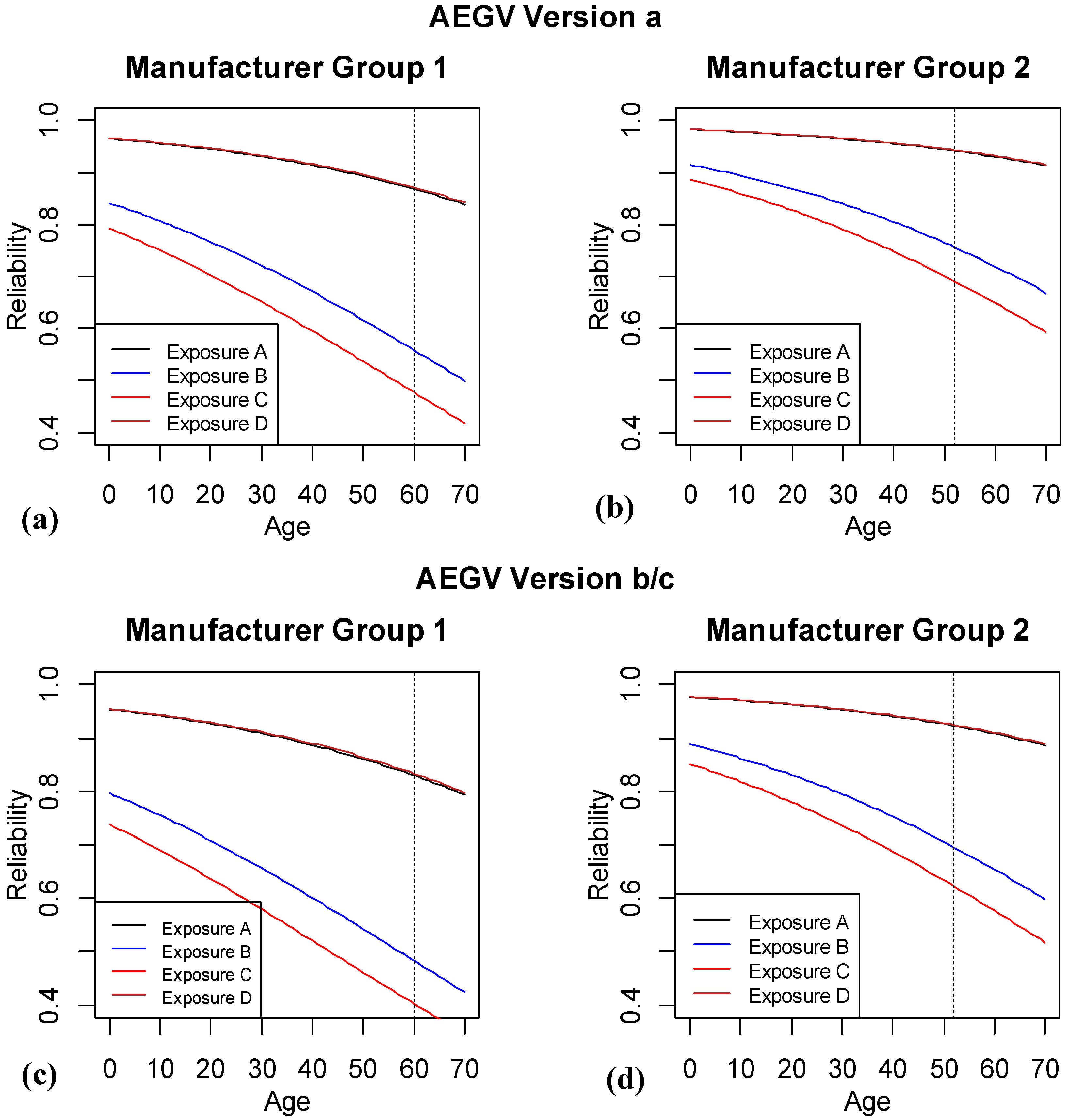
For simplicity, we next consider the 3rd and 4th best models, AEGV and AEGD, in
Figure 7 and
Figure 8, respectively. For the AEGV model, there are 24 different combinations of EGV (4(E) × 2(G) × 3(V)).
Figure 7a, b show the same eight lines combinations as
Figure 6, but this time the predictions are based on version
a of the system. For brevity and because the predictions for versions
b and
c were virtually indistinguishable, we have combined the predicted reliability plots for these two version into
Figure 7c,d.
Figure 7.
Logistic regression results with age, exposure, manufacturer group and version. The vertical dashed line highlights where the last of the observed data are available for the different subgroups of the population.
Figure 7.
Logistic regression results with age, exposure, manufacturer group and version. The vertical dashed line highlights where the last of the observed data are available for the different subgroups of the population.
The overall patterns of exposures A and D, and manufacturer 2 having higher predicted reliability continues for this model, with now the additional information that version a is predicted to have slightly higher reliability than either of version b or c.
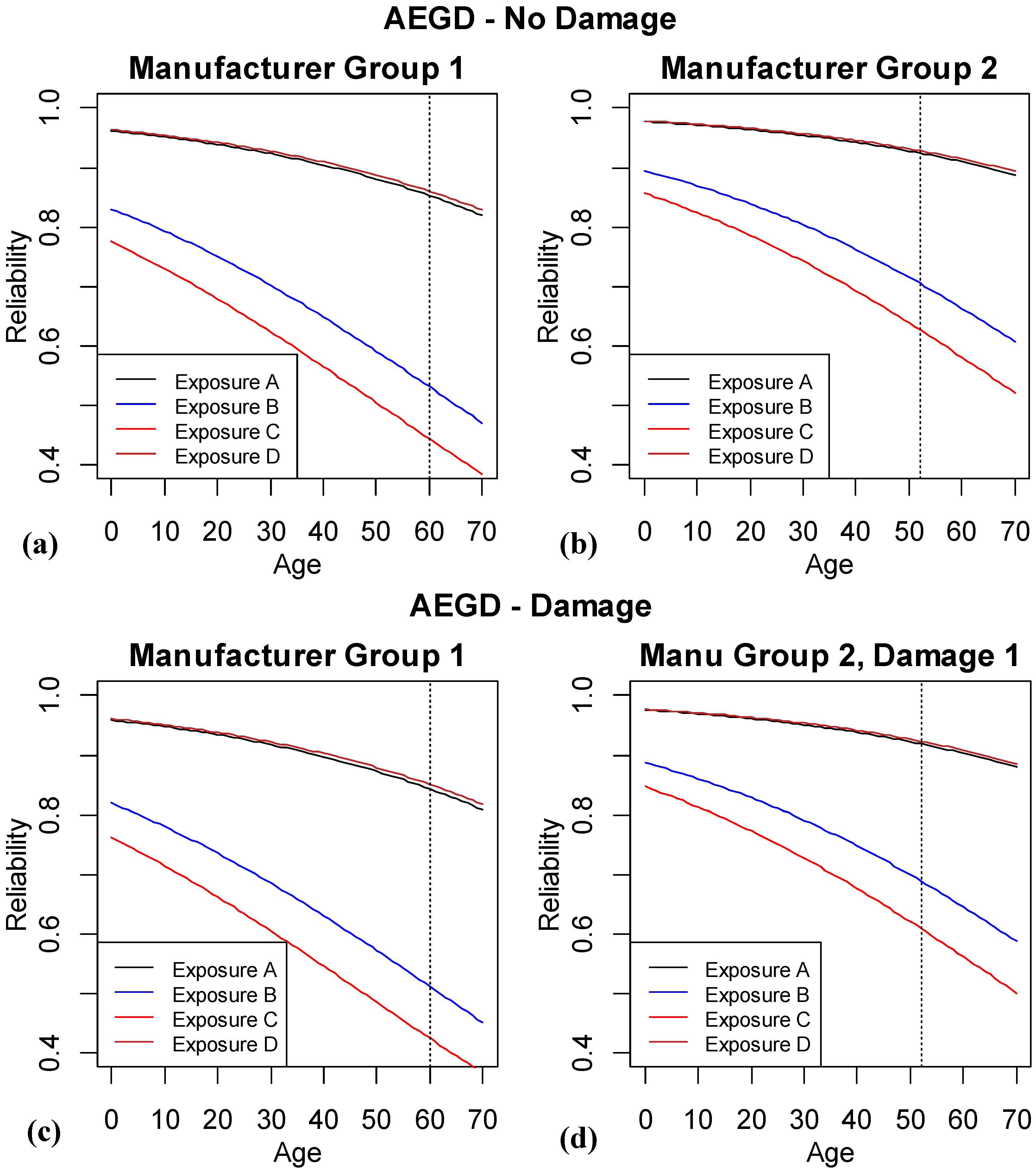
Figure 8.
Results of logistic regression model based on including age, exposure, manufacturer group and damage. The vertical dashed line highlights where the last of the observed data are available for the different subgroups of the population.
Figure 8.
Results of logistic regression model based on including age, exposure, manufacturer group and damage. The vertical dashed line highlights where the last of the observed data are available for the different subgroups of the population.
Similarly
Figure 8a,b show the same eight lines combinations as
Figure 6, but this time the predictions are based on systems with no observed superficial damage.
Figure 8c,d are the corresponding predictions when there is damage. There is minimal difference between the upper and lower plots for corresponding lines, showing that there is marginal advantage to including the superficial damage variable in the model. Since identifying superficial damage on future units is time-consuming and subjective, and superficial damage is a driver for maintenance and not a decrease in functionality, the engineers do not wish to consider this model further as a top contender.
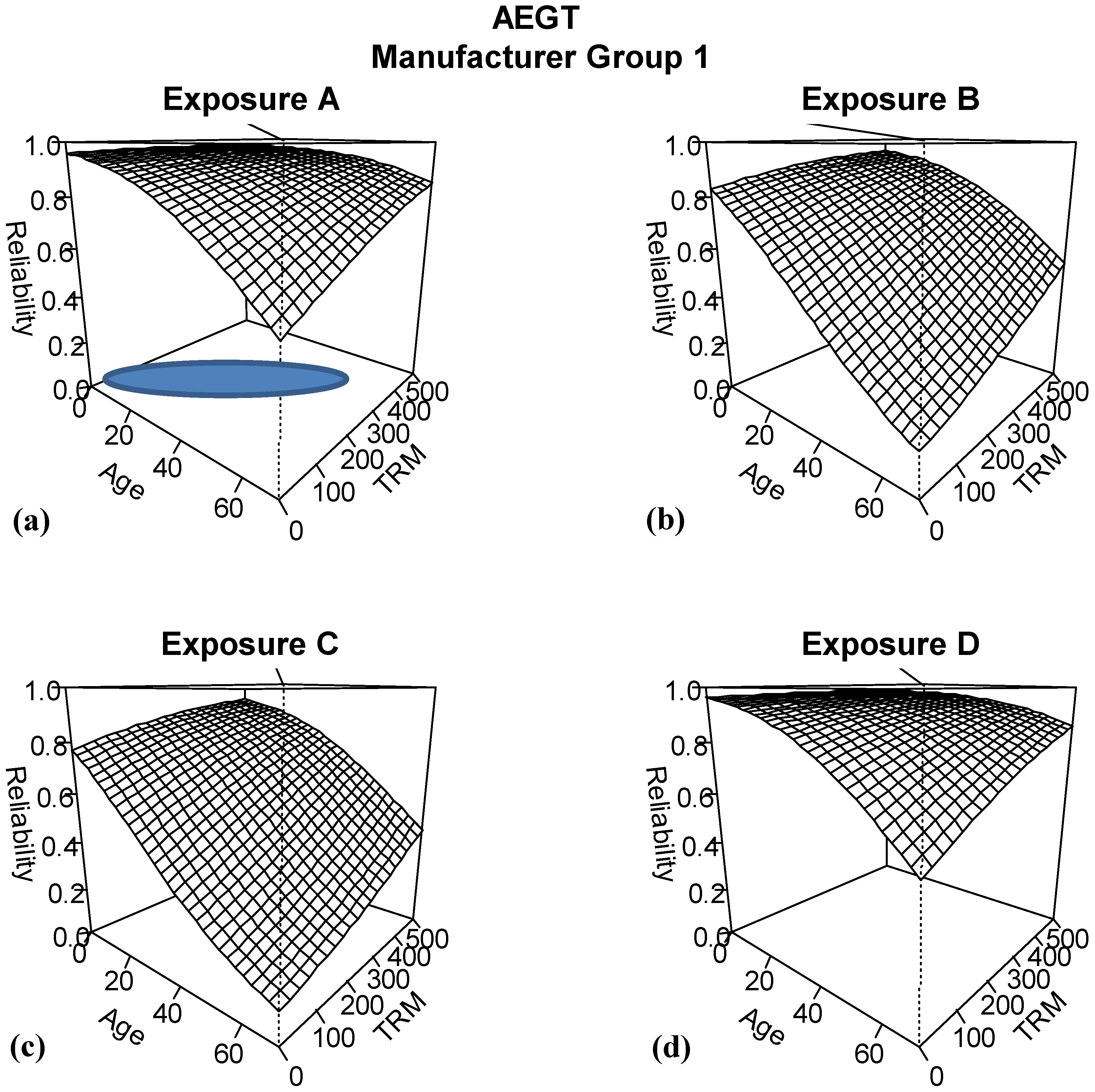
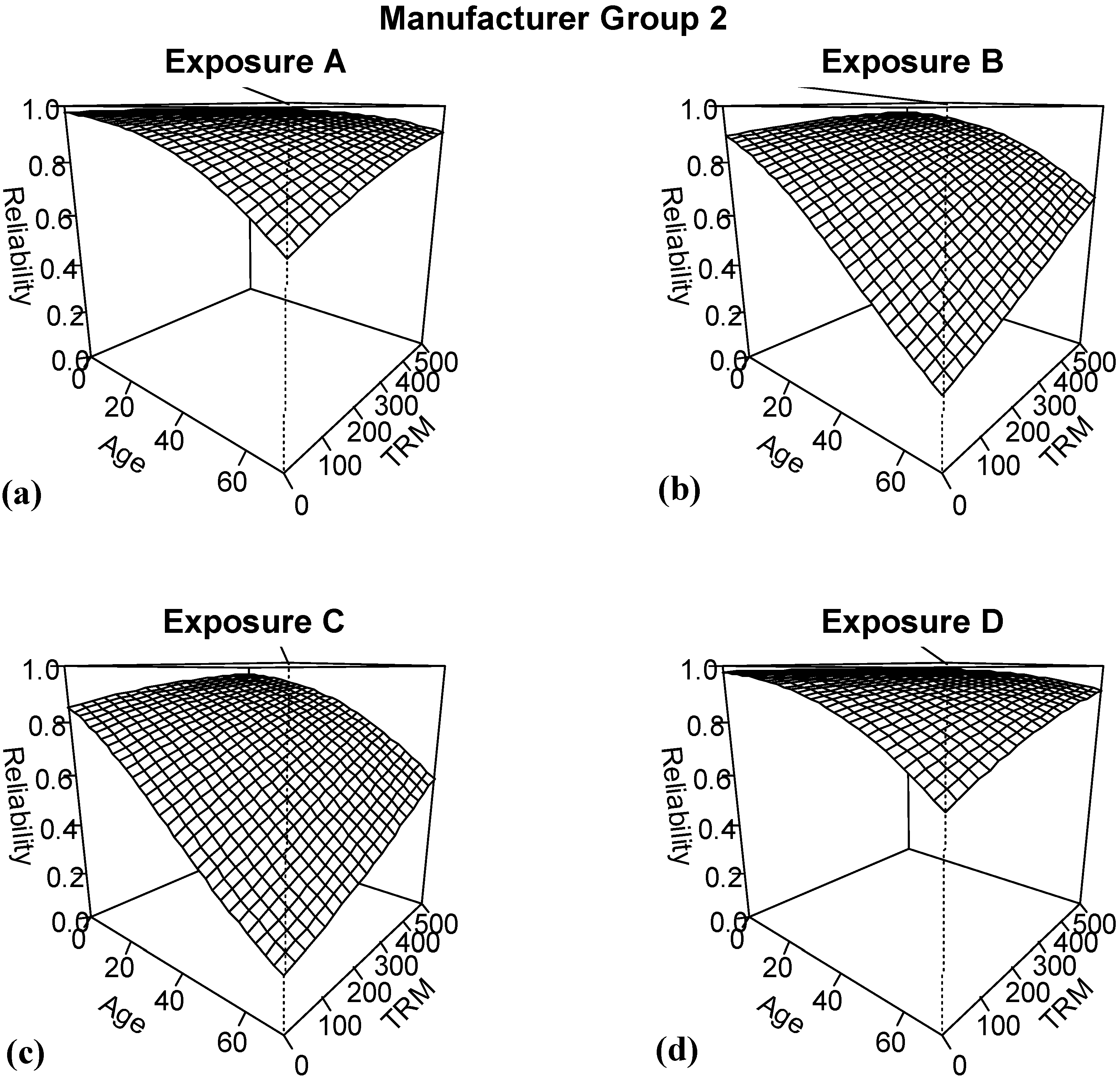
The next model considered is the second best model, AEGT. Because both age and time in ready mode are continuous variables, a different summary plot is needed to show the patterns for the different combinations of exposure and manufacturer group.
Figure 9 and
Figure 10 show surface plots of the predicted reliability for ranges of ages from 0 to 70 months and for time in ready mode ranges of 0–500 h. For each of the exposure and manufacturer group combinations, predicted reliability decreases with age. However, for a fixed age, if we increase the number of hours in time in ready mode, this is predicted to improve reliability. This is strongly counter-intuitive given current understanding of the underlying mechanism driving changes in reliability.
Figure 9.
Results of logistic regression model based on including age, exposure, manufacturer group and TRM for manufacturer group 1.
Figure 9.
Results of logistic regression model based on including age, exposure, manufacturer group and TRM for manufacturer group 1.
When we consider a possible explanation of how this result may have obtained, recall from
Section 3 and
Figure 3 that there was strong correlation between age and time in ready mode. This feature in the data has led to a common result of multicollinearity: obtaining unexpected predicted patterns in the data because of the instability of the parameter estimates. In
Figure 9a, a blue ellipse denotes where the majority of the observed data for age and time in ready mode is located. Trying to predict the reliability relationship for the entire range of age and TRM combinations from this small fraction of the space, coupled with the instability of the estimates has led to this unintuitive result. As a result, the engineers dismiss this model from further consideration.
Figure 10.
Results of logistic regression model based on including age, exposure, manufacturer group and TRM for manufacturer group 2.
Figure 10.
Results of logistic regression model based on including age, exposure, manufacturer group and TRM for manufacturer group 2.
AEGi is the final model considered; it is ranked 6th highest by AICc. This is a more complicated model based on the number of degrees of freedom in the model than the previous 4 considered. However, it has a notably smaller deviance value.
Figure 11 shows the same eight combinations of exposure and manufacturer group as
Figure 6, but this time the interaction terms allow different shapes of relationships between reliability and age for each of the combinations. For these predictions, we see that exposures A and D are no longer considered as similar, and the exposure C and MG 1 reliability curve drops very sharply.
In judging whether this additional complexity is justified, we examine the number of observations that were available to estimate each of these curves.
Table 6 shows the number of observations in each of the cell combinations. Recall that when no interactions are included in the model, the estimation leverages information for estimating the curves across different levels of the factors. When we are including more flexible interactions, then only a smaller fraction of the data are used to estimate the reliability patterns. Several of the cells in
Table 6 have relatively small numbers—in particular for exposure D. With only 42 Pass/Fail observations for combination 1 or 16 for combination 2, it is difficult to estimate the reliability pattern. Hence based on this, and that some of the drastically declining reliabilities do not match engineering understanding, this model was excluded by the experts from further consideration.
Figure 11.
Results of logistic regression model based on including age, exposure, manufacturer group and all the two-way interactions. The vertical dashed line highlights where the last of the observed data are available for the different subgroups of the population.
Figure 11.
Results of logistic regression model based on including age, exposure, manufacturer group and all the two-way interactions. The vertical dashed line highlights where the last of the observed data are available for the different subgroups of the population.
Table 6.
Number of observations in each combination of exposure and manufacturer group.
Table 6.
Number of observations in each combination of exposure and manufacturer group.
| MG/Exposure | A | B | C | D |
|---|
| 1 | 267 | 311 | 94 | 42 |
| 2 | 112 | 251 | 107 | 16 |
Of the top models examined, three were eliminated from further consideration by the subject matter experts. The second best model, AEGT, was removed because the patterns predicted for increasing TRM contradicted current understanding, and it was anticipated that this was the result of the multicollinearity issues with the data. The 4th best model, AEGD, was eliminated because the marginal potential advantage of including damage was thought to be outweighed by the time-consuming and subjective nature of collecting the data for future systems. The 6th best model, AEGi, was not considered further because its reliance on estimating reliability for some exposure and manufacturer group combinations was based on a small sample size, and because some of the predicted patterns did not match engineering understanding.
Hence the top two models at the end of this process are AEG and AEGV. The AEG model has the advantages of simplicity and being the top ranked AICc model. The third ranked AEGV model is close in AICc value, but offers the advantage of allowing a distinction to be made between the versions. It was felt that the estimated differences between versions from this model were worth tracking in the future, and this information was readily available without any additional cost. Hence the subject matter experts selected the preferred final model as AEGV. While the process for selecting the final model has subjective elements, it does follow a systematic approach and we view this as a strength of how the decision was made. A systematic approach can be anything from using a mental checklist to using a formal algorithm that emulates human decision-making. For evaluating complex systems, we are more likely to be on the less formal end of that spectrum, and while not as formal as some automated processes, this approach does incorporate considerable systematic thinking, as described by the algorithm in
Figure 1. The subject matter experts were able to see differences between the model choices, compare results with subject matter understanding of how factors are thought to impact reliability, and incorporate the cost of data collection and the associated quality of the data used for prediction. This discussion and visualization of the results helps build common understanding of the impact of factors among various engineers and scientists working on the system, and leads to deeper acceptance of the model selected. If the traditional practice of just selecting the single model with the best score on a single metric had been used, then it would have been much more difficult to obtain buy-in from the engineering community about the final choice of model.
Once a final model has been selected, it is recommended that the model assumptions be evaluated with plots of the residuals, etc. In addition, an Analysis of Variance analysis can be performed to assess formally which of the model terms are statistically significant. For this example, all of the terms in the AEGV model were statistically significant. Efforts will be made to investigate and explain differences between the different versions, as adding understanding about engineering mechanisms to the empirical results will be helpful for future predictions.
6. Conclusions
The process described in this paper allows users to efficiently consider a large number of potential explanatory variables in evaluating how to predict reliability of a system. By enumerating a list of statistical models with different combinations of the variables, the relative contributions of the variables, alone and in combination, can be quantitatively assessed. The process is flexible for different types of data, including Pass/Fail reliability data modeled with logistic regression as well as degradation data modeled with linear regression. In addition, the criterion used to evaluate the different models is flexible to match the priorities of the study.
The method is illustrated with a case study based on data with similar characteristics. One hundred and eighty-four models were fitted and ranked based on the corrected AIC (Akaike Information Criterion). The top 20 models were examined for patterns of factors included, and from this list 5 models were chosen to examine in more detail. The predicted reliability curves for different factor combinations were plotted and compared to subject matter expertise. How well the models explain patterns in the data, the match of engineering understanding with observed patterns, and the cost of obtaining future data were all considered in selecting the final overall model.
The authors feel strongly that a model selection method that identifies just a single best statistical model is too limiting. Examining several top contenders with comparable performance can help with greater understanding. In addition, when several choices are examined closely, then subject matter experts are better able to defend the choice of the top model and feel more ownership for its selection. When the process includes built-in stages where expertise and cost-effectiveness can be incorporated into the decision-making process, better results are likely. By considering different models, there is also the opportunity to translate some of the findings from the empirical study into future work for the engineers to delve into the mechanisms which led to the observed patterns in the data. This iterative process can lead to improved understanding over time, and additional confidence in the reliability predictions.
There are still opportunities or further enhancements and refinements to the outlined process. Since there are numerous different metrics that can be used to evaluate the quality of the fit of various models to the data, it would be helpful to develop a strategy for how to consider the robustness of models across different metrics, such as AIC, BIC, DIC. Advanced methods, such as least angle regression [
18], may provide algorithms for automatically searching the space of all possible models and identifying promising candidates, which provide an alternative to having the user specify the set of models under consideration. For many reliability engineers, the choice of multiple metrics that measure approximately the same thing is confusing and distracting from the task of understanding predictions from the models. We encourage a knowledgeable statistician to guide the choice of a sound statistically-based metric to use and then focus on discussions of the suitability and practicality of the model for prediction.
Since several alternative models may be identified as leading candidates, model averaging [
19] might be considered as an approach to further improve the prediction ability of the final model. One drawback of model averaging is the loss of interpretability of results, but it could be used as a gold standard against which to compare the performance of the best model. Finally, since the outlined approach can involve both continuous and categorical responses, at either the system or component levels, strategies are needed for combined model selection [
20] when multiple responses are considered. Frequently when there is interest in understanding each component or failure mode separately, decisions about which model to select are handled individually to best match with the mechanics driving reliability.


