Abstract
We present a practical guide and step-by-step flowchart for establishing uncertainty intervals for key model outcomes in a simulation model in the face of uncertain parameters. The process starts with Powell optimization to find a set of uncertain parameters (the optimum parameter set or OPS) that minimizes the model fitness error relative to historical data. Optimization also helps in refinement of parameter uncertainty ranges. Next, traditional Monte Carlo (TMC) randomization or Markov Chain Monte Carlo (MCMC) is used to create a sample of parameter sets that fit the reference behavior data nearly as well as the OPS. Under the TMC method, the entire parameter space is explored broadly with a large number of runs, and the results are sorted for selection of qualifying parameter sets (QPS) to ensure good fit and parameter distributions that are centrally located within the uncertainty ranges. In addition, the QPS outputs are graphed as sensitivity graphs or box-and-whisker plots for comparison with the historical data. Finally, alternative policies and scenarios are run against the OPS and all QPS, and uncertainty intervals are found for projected model outcomes. We illustrate the full parameter uncertainty approach with a (previously published) system dynamics model of the U.S. opioid epidemic, and demonstrate how it can enrich policy modeling results.
1. Introduction
1.1. Background and Approach
System dynamics (SD) models frequently employ parameters for which solid empirical data are not available. Modelers often use expert judgment to provide estimates of parameter values for which empirical data are not available. When several experts are available, and a formal process (such as Delphi) produces convergent estimates, modelers may have reasonable confidence in the parameter values despite the lack of data. Nevertheless, these parameter values remain uncertain to a degree—as is indeed true even for measured parameters, due to issues including small sample sizes and definitional variation.
To address parameter uncertainty, SD modelers test alternative parameter values in order to understand their degree of influence in the model. Formal sensitivity analyses can be run using features provided in popular SD software packages, and results can be displayed in a table or portrayed graphically as a “Tornado diagram” [1].
Once the modeler has identified influential parameters, additional effort is applied, as time and budget allow, to increase confidence that the values of these influential parameters are well supported. When reliable empirical data are available, ideally from multiple sources, the parameter value may be fixed and used with confidence. Usually, however, some, perhaps even many, parameter values typically remain uncertain.
This paper describes how the model analysis features available in the VensimTM software package (as well as other popular packages including Stella®), can be used to represent and incorporate parameter uncertainty into the analysis of SD model results, including providing outcome uncertainty intervals.
In this paper, we present a flowchart describing a step-by-step process for incorporating parameter uncertainty in SD models. We then illustrate use of the method using a previously published model of the U.S. opioid epidemic [2]. We close with a discussion of how model results under uncertainty can be described for interested parties such as policy makers or other end users of the analyses.
1.2. Prior Work in This Area
Ford [3] and Sterman [4] discussed uncertainty analysis vis-à-vis dynamic models. Helton et al. [5] provided a general overview of sampling-based methods for sensitivity analysis, including traditional Monte Carlo (TMC). Dogan [6,7] discussed confidence interval estimation in SD models using bootstrapping and the likelihood ratio method. Cheung and Beck [8] explained Bayesian updating in Monte Carlo processes, and background material on the mathematics of Markov Chain Monte Carlo (MCMC) is readily available [9,10].
Background on sensitivity analysis methods for dynamic modeling, and SD in particular, including the TMC and MCMC methods being employed in this paper, may be found in Fiddaman and Yeager [11], Osgood [12], Osgood and Liu [13], and Andrade and Duggan [14]. Using TMC methods to search a parameter space is sometimes considered to be a brute force or totally random search, whereas the MCMC method uses a Bayesian update process to guide the search of parameter space. In at least some contexts, it has been shown that MCMC optimally creates statistically valid samples [9].
Although publications describing the application of these methods are plentiful in some scientific and engineering disciplines, publications featuring their use with SD models are scant. A search for “system dynamics” AND (“MCMC” or “monte carlo”) returned only a handful of publications. Five relevant examples are Jeon and Chin [15], who described their use of TMC with an SD model of renewable energy; Sterman et al. [16], who applied MCMC in a model of bioenergy; Garfazadegan and Rahmandad [17] who used MCMC to estimate parameter values for a COVID-19 model, Lim et al. [18] who applied MCMC in a model of the U.S. opioid crisis; and Rahmandad et al. [19] who applied MCMC in another model of COVID-19.
2. Materials and Methods
2.1. The Process: Initial Steps
Figure 1 presents the initial steps of a process for incorporating uncertainty analysis into SD models, with further steps shown in Figure 2, Figure 3 and Figure 4. The complete process is shown in a single flowchart in Supplement Part S1.
The process starts at Create model & modify as needed. This would be a model that employs uncertain parameters and includes dynamic outcome variables that strive to match the dynamics seen in real world reference behavior data. To use the methods described in Figure 1, one needs to Define error metric variables and Add error metrics to model. A useful example could be to compute the mean absolute error (MAE) between the model calculated time series and the reference behavior time series for each outcome variable. Care must be taken to consider how to compute MAE when reference data are incomplete so as not to distort results. When different outcomes have very different scales, it is useful to use MAEM, which stands for MAE over M, where M is the mean value of the metric. In addition, composite error statistics are added to the model, such as the average of the MAEMs over all the outcomes, and the maximum value of the individual MEAMs. These are used later in the process for identifying well-fitting parameter sets. There are statistical macros available for Vensim to help with this (Supplement Part S2).

Figure 1.
Process for addressing simulation model uncertainty, initial steps.
Another initial step is to Estimate parameter uncertainty ranges, a lower and upper bound for each uncertain parameter, and to Specify weights for the outcome variables. These are needed for the algorithm used in a key part of the process: Estimate uncertain parameter values. This process employs a Powell optimization process that uses an objective function consisting of model outcomes vs. reference data. For more information, see Menzies et al. [20] for a tutorial on using Bayesian methods to calibrate health policy models. Each term of the objective function represents one of the outcome time series of interest. The algorithm strives to minimize the differences between model and reference data. Weights are needed because outcomes may have very different scales and variances. This tends to be an iterative process, so Figure 1 contains a feedback loop, and some of the connections are bidirectional. The end result of this step is a set of optimized parameter values for the uncertain parameters (OPS). Its average MAEM might be 0.1 and its maximum MAEM (worst MAEM for any one of the outcomes) might be 0.2.
2.2. The Process: Intermediate Steps for the Traditional Monte Carlo (TMC) Approach
At this point, the user may elect to use traditional Monte Carlo (TMC) or Markov Chain Monte Carlo (MCMC). TMC is discussed first; see Figure 2.
Make very large traditional Monte Carlo (TMC) run employs Vensim’s sensitivity feature to perform a very large number of model runs, millions if there are many uncertain parameters. Using this feature requires the user to specify how many runs to perform, the seed to start with, the type of sampling (e.g., multivariate, Latin hypercube, etc.), and which parameters to vary and how. We used multi-variate, which is a totally random search process. Latin hypercube strives to cover a large parameter space more efficiently. Both may be valid choices. We experimented with Uniform but settled on Triangular with the mode specified as the value from the OPS. Since we were focused on overall error, we changed the output save period (SAVEPER) to be the length of the run. This kept the output file size manageable. We also specified some additional variables to be saved (all the parameters being varied are automatically saved). These additions were the average MAEM and maximum MAEM for the run.

Figure 2.
Intermediate steps for the traditional Monte Carlo (TMC) approach.
Note that when more than one million runs are needed, we find it practical to perform one million at a time and to change the seed for each run. At the end of a sensitivity run, the data output file (.vdf in Vensim) is exported to a tab-delimited file for further analysis.
Next, the user needs to Determine cutoffs for a qualified parameter set (QPS) which involves determining how well-fitting a candidate parameter set must be to warrant its inclusion in the QPS. The vast majority of the TMC runs will not be well-fitting in the manner of the OPS. One rational approach would be to accept parameter sets that performed nearly as well as the OPS. For example, for a model in which the OPS has an average MAEM = 0.1 and the maximum MAEM = 0.2, the cutoffs for the inclusion of a candidate parameter set could be average MAEM < 0.12 and maximum MAEM < 0.25.
Sort TMC runs & create N-QPS employs Excel’s data/import external data from file to read in the TMC results. The result will be M columns by N rows, where M is the number parameters being varied + K, and N is the number of runs. K is the number of saved variables times the number of saved times per variable, which could be one, two (start time and end time), or more. The results are then sorted by average MAEM and all rows > average MAEM cutoff are discarded. The remainder is sorted by maximum MAEM and all rows > maximum MAEM are discarded. This will likely leave a very tiny fraction of runs, perhaps a few hundred out of a million. These N runs are the qualified parameter sets (N-QPS).
2.3. The Process: Intermediate Steps for Markov Chain Monte Carlo (MCMC) Approach
A very different approach for creating a set of runs to be used to evaluate the impacts of parameter uncertainty is to use the MCMC approach; see Figure 3.
This begins with Estimate Optimal Outcome Weights. First, one adds to the model a weight variable for each outcome, instead of specifying the weights numerically as in the MC process. One also needs to specify the search range for outcome weight constants. The search ranges for the uncertain parameters can be the same as for the MC approach. Or, these ranges could be broader than those used with the prior approach. No sampling distribution such as Uniform or Triangular is specified because the search of parameter space is guided by a heuristic, not by random, sampling. Guidance regarding how broad to set the ranges for MCMC varies by expert. We have heard from some, the comment that very broad ranges will give the algorithm “room to work”. Others have suggested that ranges should not include implausible values. Both comments are sensible, suggesting that a careful study of this question is needed. To proceed, first a Powell search is performed that optimizes the uncertain parameters and the weights simultaneously. In our experience, allowing larger ranges may allow the algorithm to find an optimum that achieves slightly lower average MAEM, but higher maximum MAEM. The reason is that some of the individual outcomes are sacrificed to achieve lower overall error. However, these results may be less realistic.

Figure 3.
Intermediate steps for the Markov Chain Monte Carlo (MCMC) approach.
Next is to Conduct MCMC search & generate SVS. MCMC, in the manner of MC, varies the uncertain parameters over the specified ranges, but uses in the objective function the outcome weights that were found in previous step. The Markov Chain-driven search algorithm is designed to create a statistically valid sample (abbreviated here as SVS). It can be quite large and contain many duplicates (which apparently helps to assure a sample with the correct properties). Model fitness may be further improved, but be less plausible, as mentioned earlier. Results are then exported as a tab-delimited file.
One then must Import results into Excel, and, if the population of runs produced by the MCMC search is excessively large, one can select a random sample of desired size M from the SVS. This subsample of size M, which is still a statistically valid sample (M-SVS), is comparable to the N-QPS set of runs created by the conventional MC process described earlier. One can proceed to computing statistics by parameter using the M-SVS and/or use it to run file-driven sensitivity runs, analyze alternative scenarios, etc.
2.4. The Process: Final Steps for Both TMC and MCMC
The final steps of the process are shown in Figure 4.
Save sensitivity (TMC or MCMC) parameters as a tab-delimited txt file creates the file needed for file-driven sensitivity runs.
Within Excel, the user can proceed to Compute/graph statistics by parameter to see what the values in N-QPS (or M-SVS) file are for each parameter, for example, to see if the entire range of possible values for a given parameter is represented in N-QPS, if the mean of this sample is near the value of the parameter in the OPS. Additionally, it could be used to determine the confidence interval of the estimate for the mean of the parameter based on this sample and examine the distribution (shape) of the sample. Does this information raise any red flags with respect to the OPS or N-QPS? Or, does this information indicate that the N-QPS may be representative of the entire parameter space?

Figure 4.
Final steps of the process.
Next, the N-QPS (or M-SVS) file can be used in two primary ways. One is the Run file-driven Trajectory Sensitivity Run for Baseline, for which the user can change the SAVEPER to a useful time-period, such as by year, in order to create a series of N (or M) trajectories for each outcome. The result is exported to a tab-delimited file that can be imported into Excel to Compute/graph baseline statistics by primary outcome, including uncertainty intervals for the model calculated outcome at each time period, since there is now a sample of N model-calculated values at each time point. Excel can also be used to create box and whisker plots at each time point, with or without outliers. However, we found it more expedient to create these plots using Python.
For the other primary use of the N-QPS (or M-SVS) file, explained below, the user first needs to Specify primary high-level outcomes of interest such as total cost and net performance. The previous sensitivity run was focused on behavior over time for all outcome time series, but to compare alternative scenarios in an overall sense, a few key end-of-run metrics are needed. In addition, one also needs to Specify alternative scenarios of interest; these might be different configurations or policy changes that could be implemented in the model as switches that are used in conjunction with magnitude-of-impact parameters and timing parameters linked to specific model constants.
Using the N-QPS or M-SVS, the user will change the SAVPER back to the End of Run and then Make file driven sensitivity runs for baseline and each alternative scenario. The results, for the baseline and for each scenario, are matched pairs of data points (where all of the uncertain parameter values are the same for baseline and the alternative). This means that the distributions of the differences can be used to determine, in a statistically valid fashion, the credible interval estimates (a term from Bayesian statistics), for the mean of the difference by outcome between baseline and the alternative, that can be attributed to parameter uncertainty.
We suggest that one Assemble a consolidated spreadsheet to perform these analyses. In the upper left corner, is O × N, where O is the number of overall outcomes and N is the number of runs. Note that the raw sensitivity results file has columns for all the parameters as well as columns for each outcome. The user selects and copies only the end columns for each outcome into the consolidated sheet. The data for Alternative 1 is placed below the Baseline results; Alternative 2 below Alternative 1, etc. Then, starting at the first row of Alternative 1, columns will be added to compute the differences between the Alternative 1 numbers and baseline number, one column for each outcome. Similarly for Alternative 2 vs. baseline, and so forth. Columns for percentage differences can also be added.
Finally, Create summary table(s) or tab(s) is used to provide the results of relevant calculations, such as means and their credible intervals for each outcome at baseline and for each alternative. In addition, the results for the differences by outcome between baseline and Alternative 1, baseline and Alternative 2, etc., may be compiled. Similarly, for the percentage differences.
2.5. About the Opioid Epidemic Model
To illustrate the process and results, the TMC method was applied to an SD model of significant complexity that explored the opioid epidemic in the United States from 1990 to 2030 including the impacts of alternative policies (hereafter the Opioid Epidemic Model) [2,21]. SD has been frequently applied to drug abuse and other areas of public health and social policy [22,23,24,25,26]. The current model adopts the basic scientific approach and some of the same elements as these forerunner models, but the current model was completely redeveloped to address current needs.
A committee of the National Academies of Sciences/Engineering/Medicine considered the complexities of the opioid epidemic and stated that for informed decision making “a true systems model, not just simple statistics” was needed because “decisions made about complex systems with endogenous feedback can be myopic in the absence of a formal model” [27]. The NAS cited the system dynamics model by Wakeland et al. [24] as an example of a true systems model.
Best practices for model development, testing, and reporting are well documented [4,28,29,30]. The model building process for the Opioid Epidemic Model involved amassing evidence from many different sources and developing a dynamic structure that reproduces historical trends and is sufficiently parsimonious to allow explanation. Uncertainties are addressed through sensitivity testing and the multivariate TMC testing described previously that allows results to be reported with rigorous credible intervals.
A complete list of the approximately 340 interacting model equations (including about 80 input constants, 17 time series for input and validation, and 240 output variables) is available in the model’s reference guide [21]. This guide also provides stock and flow diagrams for each sector of the model and describes how model constants and time series were estimated, including data sources. The model time horizon was 1990–2030. Figure 5 shows the basic model structure.
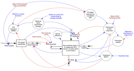
Figure 5.
Opioid Epidemic Model diagram showing high level stocks, flows, and primary feedback structures. Red lines are causal links with negative valence, while blue lines have positive valence. Reproduced by permission from Homer and Wakeland 2020 [2].
3. Results
3.1. Error Metrics
As the first step in the TMC approach, error metrics were created, in this case, MAEM (mean absolute error over mean) for multiple outcome time series with historical data counterparts. We used the Vensim SSTATS macro provided by Professor John Sterman at MIT; see Supplement Part S2. This code was inserted via text editor (we used Notepad) at the top of the model file starting at the second line. Supplement Part S3 presents the model code for calculating the statistics, which was also inserted into the model file via text editor, typically after the Control block, which is located after the user-defined model variables/constants section. We utilized an Excel workbook that included a worksheet with Time in Row 1 and historical time series data in the rows below. In some cases, there were data only for some of the historical years. The SSTATS macro calculations are designed to handle this correctly. An example Vensim equation for reading one these data time series is GET XLS DATA (‘model RBP data.xlsx’, ‘RBP’, ‘1’, ‘B2’).
Another step to prepare the model for analysis was to add a custom graphs file via the Control Panel and add custom tables that display the variables calculated by the SSTATS macro (R2, MAPE, MAEM, RMSE, Um, Us, Uc, and Count), one table for each Outcome variable. I/O Objects were added to a model view to display the custom tables.
Figure 6 shows a sample of these statistical parameter displays created using the SSTATS macro, with the MAEM statistics on the left and R-squared statistics on the right. These outputs were from the optimized parameter set (OPS) version of the Opioid Epidemic Model; see discussion below. In addition to the weighted average of all the MAEMs of 8.9% (bottom left 2020 column), it is clear that OD death-related trajectories were reproduced more accurately than, for example, heroin-related trajectories. The MAEM for OD deaths total was 3.6%, whereas for H initiates it was 18%. This large difference was due mostly to noise in the data representing the actual values. OD death data are the actual data collected by the CDC, and the changes from year to year are modest. Data on persons initiating heroin in a given year is based on a small sample of a difficult-to-access population and the resulting estimates by year vary dramatically. In fact, the difference between the data and the corresponding three-period moving average was 12.5%, suggesting that most (70%) of the 18% model-calculated MAEM was due to noise in the data.
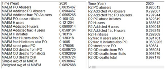
Figure 6.
Selected SSTATS displays (MAEM and R-squared for outcome variables).
3.2. Optimized Parameter Set (OPS)
Before using optimization to estimate uncertain parameter values, the user must specify an appropriate range for each parameter to be used by the Powell search algorithm. Supplement Part S4 provides an example Vensim optimization control file (.voc) which specified the uncertain parameters to be varied. Table 1 shows the first few rows of the model parameter spreadsheet by parameter, including the minimum and maximum values. Many of the 80 model parameters had empirical support from the literature, which helped to reduce the uncertainty ranges for these parameters.

Table 1.
Portion of the opioid model parameter spreadsheet showing parameter name, units, value (central estimate), source (or optimized), and the minimum and maximum values used during optimization runs.
In addition, weights must be specified for the objective function, informed by the relative magnitudes and variances of the outcome variables. In this example, weights were set so that metrics with solid empirical data were given more weight than those for which empirical data were scant or less reliable.
The optimization runs using the CG (calibration Gaussian) option ran for several minutes on a laptop computer. A blend of modeler judgment and optimization results was used iteratively to select the values for the optimized parameter set. The MAEMs for many of the outcomes were reduced compared with a purely manual calibration process. The weighted (based on the amount of data available for each outcome) average of the MAEMs was 8.9%, with the largest individual MAEM being 17.9%.
Figure 7 shows the trajectories for two example outcomes calculated by the model using the optimized parameter set compared with the available historical data for these metrics. The MAEMs for the two outcomes in Figure 7 were 9% and 4%. The calculated Persons with Addiction trajectory was somewhat biased downward, whereas the OD Deaths trajectory matched very well. One possible reason could be the amount of data available: the standardized errors for the first variable may carry somewhat less weight than the second one. Additionally, note that measurement uncertainty was greater for the first variable than the second one.

Figure 7.
Model fit to two key outcomes using the optimized parameter set.
3.3. Qualified Parameter Sets (N-QPS)
Creating a large Monte Carlo run is easy using the sensitivity feature in Vensim, which uses or creates a .vsc file. One option for exploring parameter space could be to use Uniform distributions between thoughtfully chosen minima and maxima. These values could be the same as those used during calibration, or perhaps narrowed somewhat. Another option could be to use a Triangular distribution with the optimum value as the mode, which would increase samples near the optima. For this illustration, Triangular distributions were used. The user also needs to specify a .lst file that lists which variables are to be saved for each run. Sensitivity runs automatically save the varied parameters used for each run, and in addition, it is useful to know the maximum MAEM and average MAEM (to be used to select which runs are qualified). Since we do not need to know the time trajectories, we set the model SAVEPER to 40. This kept the output file modest in size. Supplement Part S5 shows the .vsc and .lst files.
The simulation was set to create one million runs, which took about seven hours on a laptop. Ten such runs were made, changing the random seed for each run, creating a total sample of ten million runs. Each resulting data output file (.vdf) was exported (via the model menu) to a tab-delimited file and read into Excel using data/get external data/from text (switch to All Files to see .tab files). This was sorted by weighted average of MAEMs. The weighted average MAEM was below 0.11 for 300–600 runs in each of the one million runs, and these rows were kept. The other rows were deleted.
The file was then sorted by maximum MAEM, and 100–130 runs were less than 0.20 and kept. The rest were deleted. These ten spreadsheets were combined, yielding a sample of 1119 runs that accomplished <11% weighted average error and <20% maximum error. Rows were added below the sample to calculate useful statistics about the sample, regarding both the distributions of the input parameters and the how well each run performed. Table 2 shows the first and last few rows of the spreadsheet.
Table 2.
First and last few rows and columns of the file used to create the N-QPS.
We next examined the properties of the parameter samples contained in the N-QPS. The rows at the bottom of Table 2 show the minimum, maximum, mean, and standard deviation of each parameter. For more detail, histogram plots were created, with examples shown in Figure 8. The parameter shown on the left, Addicted PONHA move to heroin rate initial, was limited to be in the 0.01 to 0.03 range. As the histogram shows, nearly all of this allowed range was included in the N-QPS. The mode was about 0.0235, which was slightly higher than its value of 0.021 in the optimized parameter set. The parameter on the right, Consumption mgs ME per addicted PO abuser per month initial, was limited to be in the range of 2000 to 5000; the values in the N-QPS were well inside these limits (2092 to 4566). The mode was 3330, very slightly higher than its value of 3200 in the optimized parameter set. One can examine all of the parameter histograms in this fashion to build confidence in the sample.
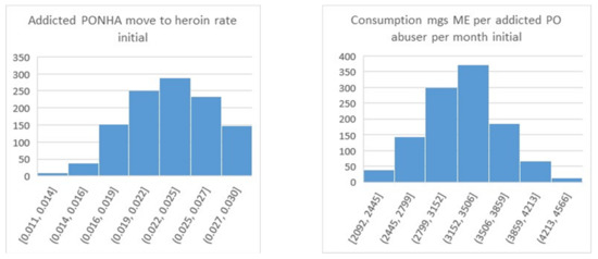
Figure 8.
Histograms for two uncertain parameters resulting from the TMC approach.
For comparison, Figure 9 shows a histogram that results from using the MCMC algorithm rather than TMC, again considering the parameter that was on the left side of Figure 8. For MCMC, nearly all of the samples fell in the range from 0.02 to 0.0216 with a width of 0.0016, whereas the range for same parameter in Figure 8 is from 0.014 to 0.03 with a width of 0.026 (greater by 16x), and the shape has a sharp rather than rounded peak. We found that nearly all of the parameter distributions from testing MCMC on the Opioid Epidemic Model had this narrow and pointed characteristic. The problem was not skewness, but the implausibly high degree of precision in the estimated parameter value, within just a few percentage points.
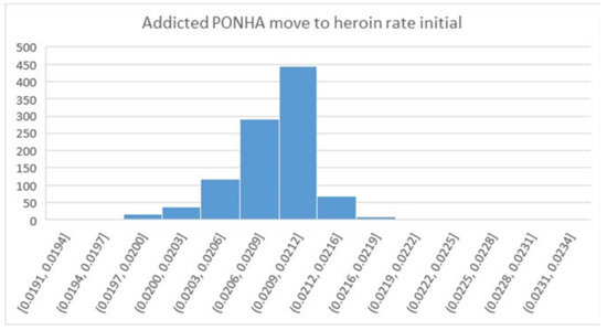
Figure 9.
Histogram for an uncertain parameter resulting from the MCMC approach. Note that all of the bars in this diagram are contained within the fourth bar on the left side of Figure 8.
Using different settings for the MCMC algorithm yielded similar very narrow and pointed samples, prompting the decision to rely on the TMC-based method that tests a much broader range of potential values for these parameters. However, other researchers have reported successful use of the MCMC method [15,16,17,18,19], indicating that the MCMC approach may be preferred in many cases.
3.4. Sensitivity Runs for the Baseline Scenario
To put the N-QPS sample from the MC-based method to use, file-driven sensitivity runs were performed. The SAVEPER was changed to 40, and the Sensitivity tool was selected. Previous settings were cleared, and the Type of sensitivity run was changed to File. The N-QPS text file was selected as the file. Next a save list was created. The previous save list (with the statistical variables) was cleared, and three primary outcome variables were entered: Total opioid addicts, Opioid overdoses seen at ED, and Total opioid OD deaths. This run took just a minute to complete, and the data output file (.vdf) it produced was exported via Vensim and imported into Excel.
The first 50 columns of this trajectory spreadsheet provided the run number (1–1119) and the values of the 49 uncertain parameter values used for each specific run. The remaining 41 columns were values from time 1990 to 2030 for the three outcome variables. Figure 10 shows the trajectory under uncertainty for Overdoses Seen at ED using a box-and-whiskers plot. One can also use the data in the spreadsheet to report useful sample statistics, such as mean and standard deviation.
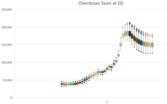
Figure 10.
Excel box-and-whisker time series plot for Overdoses Seen at ED under the baseline scenario.
Unfortunately, there was no easy way using Excel to superimpose the historical data on this plot. Python software could be used to create such a plot as needed. Figure 11 shows the plot produced using Python for Total opioid OD deaths, showing the credible interval trajectory overlaid with green dots for the historical data. The credible interval was similar in spirit to the confidence intervals used to characterize statistical samples from actual populations.
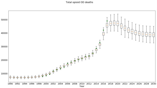
Figure 11.
Python box-and-whisker time series plot for Total Opioid OD Deaths under the baseline scenario, overlaid with historical data (green dots).
To prepare the file needed by Python, a version of the trajectory spreadsheet was created, named Outcome Trajectory Data for Python Plotting (OTDPP), in which the columns for run number and the parameter values were deleted. Additionally, two rows were added below the first row. Row 2 should contain the actual data to be overlaid. For each outcome variable, the appropriate row of the RBP spreadsheet was copied above its corresponding section in OTDPP. Since the RBP data spreadsheet contained up to 30 values of historical data for each outcome trajectory, and since the data sections for each outcome in OTDPP were oriented horizontally, it was a simple copying process, even for several outcomes. Row 3 in OTDPP should provide the time values, which was easily created in Excel or could be copied from the historical data spreadsheet (41 cells copied once and pasted N times in the OTDPP, where N is the number of outcome variable, 3 for this example).
3.5. Sensitivity Runs for Alternative Scenarios (Policy Testing under Uncertainty)
Another use of the N-QPS is to compare a baseline case with policy runs, to determine how much impact parameter uncertainty may have with respect to the most important outcome indicators. In the case of the Opioid Epidemic Model, three key indicators were the number of people with opioid addiction (also known as opioid use disorder or OUD), opioid overdose events, and opioid overdose deaths. These metrics are saved for each of the parameter sets in the N-QPS, for the baseline condition and for each alternative. The net change in outcome, and policy vs. baseline, were calculated run by run, in both absolute and percentage terms.
The Opioid Epidemic Model was run using the file-driven sensitivity tool reading in the 1119-QPS parameter sets, and for five potential policies aside from the baseline. The final values for the three key metrics were saved for each of the 1119 runs, and a spreadsheet was created to compute the differences in outcome metrics, run by run. This spreadsheet had 1119 rows and 48 columns. The first three columns were the final baseline values for each of the three metrics. Then, nine columns were created for each of the five policies. These were the three columns of raw outcomes, plus three columns that calculated the change, and three more that calculated the percentage change. A row was added at the bottom to compute the mean percentage change in each outcome due to each policy. Two more rows computed minimum change in each metric and the maximum change in each metric.
Table 3 presents a summary of the parameter uncertainty analysis of the impacts of the various policies. The % change vs. Baseline under OPS may be compared with the Mean %Δ and the range (min, max) of percentage changes under the QPS 1119. Even though the mean of the QPS-driven change was generally close to the results using the OPS, seeing the uncertainty interval provides more information to inform policy decisions. Three examples are highlighted in yellow, as follows:
- Treatment rate 65% (from 45%) policy and the outcome Persons with OUD: The model projected a modest unfavorable impact for the OPS and a modest favorable impact for the QPS. The QPS sample interval contained zero, so this policy should perhaps be considered not to impact Persons with OUD;
- All four policies combined and the outcome Overdoses Seen at ED: a mean beneficial outcome was predicted by both, but the credible interval again included zero, indicating that the net effect of all four policies on overdose events could be neutral;
- Diversion control policy and the outcome OD Deaths: The uncertainty interval again included zero, suggesting that for a significant number of the qualified parameter sets, the impact was unfavorable. This was likely due to persons switching to more dangerous drugs. This hypothesis could be examined directly by studying the uncertainty analysis results to find the specific parameter values which render the policy ineffective.
Table 3.
Impact of parameter uncertainty on the simulated results of policy changes.
Table 3.
Impact of parameter uncertainty on the simulated results of policy changes.
| Optimized Parameter Set | QPS 1119 MC Result | QPS 1119 MC, % Change vs. Baseline | |||||||
|---|---|---|---|---|---|---|---|---|---|
| Outcome Measure | Test Condition | Result | % Change vs. Baseline | Mean | Credible Interval | Mean %Δ | Credible Interval | ||
| Min | Max | Min | Max | ||||||
| Persons with OUD (thou) | Baseline | 1694 | 1593 | 1111 | 2084 | ||||
| Avg MME dose down 20% | 1510 | −10.9% | 1416 | 1035 | 1823 | −11.1% | −25.7% | −3.4% | |
| Diversion Control 30% | 1428 | −15.7% | 1339 | 1007 | 1716 | −15.9% | −37.4% | −4.6% | |
| Treatment rate 65% (from 45%) | 1713 | 1.1% | 1585 | 1054 | 2130 | −0.5% | −9.0% | 5.0% | |
| Naloxone lay use 20% (from 4%) | 1728 | 2.0% | 1624 | 1150 | 2111 | 1.9% | 1.3% | 2.3% | |
| All four policies combined | 1285 | −24.1% | 1189 | 905 | 1560 | −25.4% | −60.2% | −6.5% | |
| Overdoses seen at ED (thou) | Baseline | 155 | 149 | 124 | 179 | ||||
| Avg MME dose down 20% | 153 | −1.3% | 145 | 118 | 176 | −2.7% | −8.2% | 3.8% | |
| Diversion Control 30% | 153 | −1.1% | 144 | 116 | 175 | −3.4% | −11.6% | 6.0% | |
| Treatment rate 65% (from 45%) | 150 | −3.0% | 144 | 118 | 171 | −3.7% | −11.3% | −0.3% | |
| Naloxone lay use 20% (from 4%) | 159 | 2.9% | 154 | 128 | 187 | 3.1% | 2.2% | 5.1% | |
| All four policies combined | 148 | −4.1% | 139 | 111 | 168 | −7.3% | −19.6% | 6.1% | |
| Overdose deaths (thou) | Baseline | 40.3 | 39.0 | 32.5 | 46.7 | ||||
| Avg MME dose down 20% | 39.8 | −1.3% | 37.9 | 30.9 | 46.0 | −2.7% | −8.2% | 0.6% | |
| Diversion Control 30% | 39.9 | −1.1% | 37.6 | 30.3 | 45.5 | −3.4% | −11.6% | 6.0% | |
| Treatment rate 65% (from 45%) | 39.2 | −3.0% | 37.5 | 30.8 | 44.6 | −3.7% | −11.3% | −0.3% | |
| Naloxone lay use 20% (from 4%) | 35.3 | −12.5% | 34.2 | 28.4 | 41.4 | −12.3% | −18.6% | −8.1% | |
| All four policies combined | 32.9 | −18.4% | 30.7 | 24.5 | 31.2 | −21.1% | −36.4% | −6.9% | |
4. Discussion
Here we have demonstrated a practical method for analyzing the effects of parameter uncertainty on simulated model projections, using a health policy example. The process summarized in Figure 1, Figure 2, Figure 3 and Figure 4 (and Supplement Part S1) provides two alternative approaches: traditional Monte Carlo (TMC) and Markov Chain Monte Carlo (MCMC). We featured the former in this paper, because of its greater familiarity and ease of understanding.
However, it should be noted that, despite our difficulties with MCMC (specifically, the overly narrow parameter distributions we observed), it is the theoretically superior and less time-consuming of the two approaches. Tom Fiddaman at Ventana Systems (the makers of Vensim) has suggested that a better choice of likelihood function for MCMC might have produced better dispersed parameter distributions.
Indeed, other research teams have had success with MCMC [15,16,17,18,19]. Although MCMC yields theoretically superior results, further examination and characterization of the parameter distributions resulting from MCMC seems to be in order. Garfazadegan and Rahmandad [17] note in their Appendix A “rather tight confidence intervals coming from MCMC methods directly applied to large nonlinear models,” which they address via heuristics that scale the likelihood function.
A possible limitation of both TMC and MCMC is their reliance on the goodness of fit to historical data. Forrester [32] warned that “the particular curves of past history are only a special case.” The implication is that this method should not be used to make claims of precision in predicted outcomes, but rather to better appreciate the range of possible outcomes and, especially, the uncertainty in projected policy impacts.
5. Conclusions
We have presented a step-by-step approach to assessing the degree of uncertainty in simulation model outcomes related to uncertainty in the model’s input parameters. Our flowchart summarizes two ways to perform this, and we have demonstrated one of these in detail with a concrete health policy example. Providing uncertainty intervals for the range of possible outcomes from contemplated policy options, as we have described here, could increase the value of simulation models to decision makers.
Supplementary Materials
The following supporting information can be downloaded at: https://www.mdpi.com/article/10.3390/systems10060225/s1, Supplement Part S1: Complete process for addressing simulation model uncertainty (uniting Figures S1 to S4) and Supplement Parts S2 to S5.
Author Contributions
W.W. and J.H. have met authorship requirements, and contributed to every part of the manuscript. All authors have read and agreed to the published version of the manuscript.
Funding
The original Opioid Epidemic Model was developed under contract in 2019 (see [2]), but the uncertainty analysis described here was performed subsequently and received no funding.
Institutional Review Board Statement
Not applicable.
Informed Consent Statement
Not applicable.
Data Availability Statement
All data presented in this article were extracted from publicly available data sources (see [2]).
Acknowledgments
The authors wish to thank Kevin Stoltz who wrote the Python code for graphing uncertainty interval time series, as well as John Sterman and Tom Fiddaman for their advice.
Conflicts of Interest
The authors declare no conflict of interest.
References
- Wakeland, W.; Hoarfrost, M. The case for thoroughly testing complex system dynamics models. In Proceedings of the 23rd International Conference of the System Dynamics Society, Boston, MA, USA, 17–21 July 2005. [Google Scholar]
- Homer, J.; Wakeland, W. A dynamic model of the opioid drug epidemic with implications for policy. Am. J. Drug Alcohol. Abuse. 2020, 47, 5–15. [Google Scholar] [CrossRef] [PubMed]
- Ford, A. Estimating the impact of efficiency standards on the uncertainty of the northwest electric system. Oper. Res. 1990, 38, 580–597. [Google Scholar] [CrossRef]
- Sterman, J.D. Business Dynamics: Systems Thinking and Modeling for a Complex World; Irwin McGraw-Hill: Boston, MA, USA, 2000. [Google Scholar]
- Helton, J.C.; Johnson, J.D.; Sallaberry, C.J.; Storlie, C.B. Survey of sampling-based methods for uncertainty and sensitivity analysis. Reliab. Eng. Syst. Saf. 2006, 91, 1175–1209. [Google Scholar] [CrossRef]
- Dogan, G. Confidence interval estimation in system dynamics models: Bootstrapping vs. likelihood ratio method. In Proceedings of the 22nd International Conference of the System Dynamics Society, Oxford, UK, 25–29 July 2004. [Google Scholar]
- Dogan, G. Bootstrapping for confidence interval estimation and hypothesis testing for parameters of system dynamics models. Syst. Dyn. Rev. 2007, 23, 415–436. [Google Scholar] [CrossRef]
- Cheung, S.H.; Beck, J.L. Bayesian model updating using hybrid Monte Carlo simulation with application to structural dynamic models with many uncertain parameters. J. Eng. Mech. 2009, 135, 243–255. [Google Scholar] [CrossRef]
- Ter Braak, C.J.F. A Markov Chain Monte Carlo version of the genetic algorithm Differential Evolution: Easy Bayesian computing for real parameter spaces. Stat. Comput. 2006, 16, 239–249. [Google Scholar] [CrossRef]
- Vrugt, J.A.; ter Braak, C.J.F.; Diks, C.G.H.; Robinson, B.A.; Hyman, J.M.; Higdon, D. Accelerating Markov Chain Monte Carlo Simulation by differential evolution with self-adaptive randomized subspace sampling. Int. J. Nonlinear Sci. Numer. Simul. 2009, 10, 271–288. [Google Scholar] [CrossRef]
- Fiddaman, T.; Yeager, L. Vensim calibration and Markov Chain Monte Carlo. In Proceedings of the 33rd International Conference of the System Dynamics Society, Cambridge, MA, USA, 19–23 July 2015. [Google Scholar]
- Osgood, N. Bayesian parameter estimation of system dynamics models using Markov Chain Monte Carlo methods: An informal introduction. In Proceedings of the 31st International Conference of the System Dynamics Society, Cambridge, MA, USA, 21–25 July 2013. [Google Scholar]
- Osgood, N.D.; Liu, J. Combining Markov Chain Monte Carlo approaches and dynamic modeling. In Analytical Methods for Dynamic Modelers; Rahmandad, H., Oliva, R., Osgood, N.D., Eds.; MIT Press: Cambridge MA, USA, 2015; Chapter 5; pp. 125–169. [Google Scholar]
- Andrade, J.; Duggan, J. A Bayesian approach to calibrate system dynamics models using Hamiltonian Monte Carlo. Syst. Dyn. Rev. 2021, 37, 283–309. [Google Scholar] [CrossRef]
- Jeon, C.; Shin, J. Long-term renewable energy technology valuation using system dynamics and Monte Carlo simulation: Photovoltaic technology case. Energy 2014, 66, 447–457. [Google Scholar] [CrossRef]
- Sterman, J.D.; Siegel, L.; Rooney-Varga, J.N. Does replacing coal with wood lower CO2 emissions? Dynamic lifecycle analysis of wood bioenergy. Environ. Res. Lett. 2018, 13, 015007. [Google Scholar] [CrossRef]
- Ghaffarzadegan, N.; Rahmandad, H. Simulation-based estimation of the early spread of COVID-19 in Iran: Actual versus confirmed cases. Syst. Dyn. Rev. 2020, 36, 101–129. [Google Scholar] [CrossRef]
- Lim, T.Y.; Stringfellow, E.J.; Stafford, C.A.; DiGennaro, C.; Homer, J.B.; Wakeland, W.; Jalali, M.S. Modeling the evolution of the US opioid crisis for national policy development. Proc. Natl. Acad. Sci. USA 2022, 119, e2115714119. [Google Scholar] [CrossRef]
- Rahmandad, H.; Lim, T.Y.; Sterman, J. Behavioral dynamics of COVID-19: Estimating underreporting, multiple waves, and adherence fatigue across 92 nations. Syst. Dyn. Rev. 2021, 37, 5–31. [Google Scholar] [CrossRef]
- Menzies, N.A.; Soeteman, D.I.; Pandya, A.; Kim, J.J. Bayesian methods for calibrating health policy models: A tutorial. Pharmacoeconomics 2017, 35, 613–624. [Google Scholar] [CrossRef]
- Homer, J. Reference Guide for the Opioid Epidemic Simulation Model (Version 2u); February 2020. Available online: https://pdxscholar.library.pdx.edu/cgi/viewcontent.cgi?filename=0&article=1154&context=sysc_fac&type=additional (accessed on 7 November 2022).
- Levin, G.; Roberts, E.B.; Hirsch, G.B. The Persistent Poppy: A Computer-Aided Search for Heroin Policy; Ballinger: Cambridge, MA, USA, 1975. [Google Scholar]
- Homer, J.B. A system dynamics model of national cocaine prevalence. Syst. Dyn. Rev. 1993, 9, 49–78. [Google Scholar] [CrossRef]
- Homer, J.; Hirsch, G. System dynamics modeling for public health: Background and opportunities. Am. J. Public Health 2006, 96, 452–458. [Google Scholar] [CrossRef]
- Wakeland, W.; Nielsen, A.; Schmidt, T.; McCarty, D.; Webster, L.; Fitzgerald, J.; Haddox, J.D. Modeling the impact of simulated educational interventions in the use and abuse of pharmaceutical opioids in the United States: A report on initial efforts. Health Educ. Behav. 2013, 40, 74S–86S. [Google Scholar] [CrossRef]
- Wakeland, W.; Nielsen, A.; Geissert, P. Dynamic model of nonmedical opioid use trajectories and potential policy interventions. Am. J. Drug Alcohol. Abuse 2015, 41, 508–518. [Google Scholar] [CrossRef]
- Bonnie, R.J.; Ford, M.A.; Phillips, J.K. (Eds.) Pain Management and the Opioid Epidemic: Balancing Societal and Individual Benefits and Risks of Prescription Opioid Use; National Academies Press: Washington, DC, USA, 2017. [Google Scholar]
- Homer, J.B. Why we iterate: Scientific modeling in theory and practice. Syst. Dyn. Rev. 1996, 12, 1–19. [Google Scholar] [CrossRef]
- Richardson, G.P. Reflections on the foundations of system dynamics. Syst. Dyn. Rev. 2011, 27, 219–243. [Google Scholar] [CrossRef]
- Rahmandad, H.; Sterman, J.D. Reporting guidelines for system dynamics modeling. Syst. Dyn. Rev. 2012, 8, 251–261. [Google Scholar]
- Ray, W.A.; Chung, C.P.; Murray, K.T.; Hall, K.; Stein, C.M. Prescription of long-acting opioids and mortality in patients with chronic noncancer pain. JAMA 2016, 315, 2415–2423. [Google Scholar] [CrossRef] [PubMed]
- Forrester, J.W. System dynamics—The next fifty years. Syst. Dyn. Rev. 2007, 23, 359–370. [Google Scholar] [CrossRef]
Publisher’s Note: MDPI stays neutral with regard to jurisdictional claims in published maps and institutional affiliations. |
© 2022 by the authors. Licensee MDPI, Basel, Switzerland. This article is an open access article distributed under the terms and conditions of the Creative Commons Attribution (CC BY) license (https://creativecommons.org/licenses/by/4.0/).