Algorithms for Computing the Triplet and Quartet Distances for Binary and General Trees

Abstract
:1. Introduction
2. The Triplet and Quartet Distances
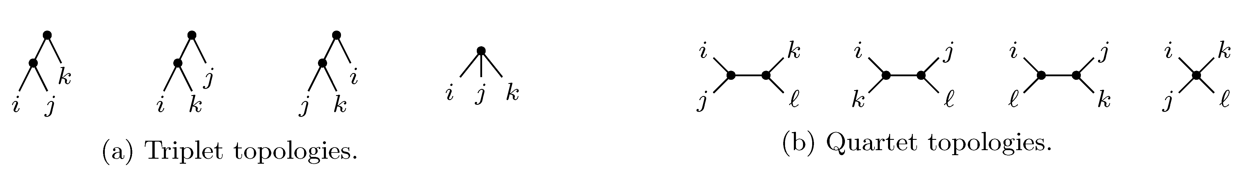
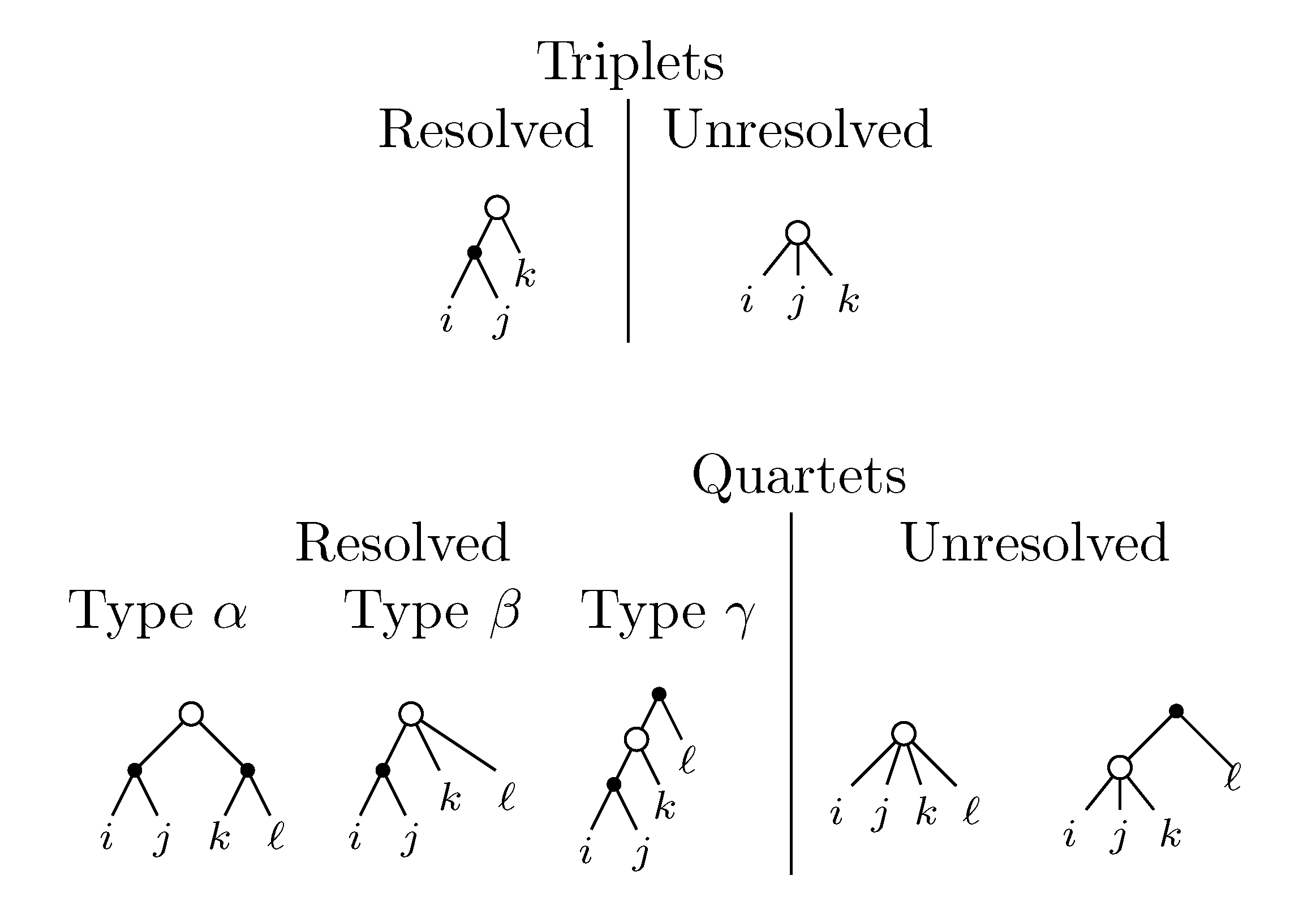
 sets of three leafs and for each set comparing the induced topologies in the two trees.
 sets of four leafs and for each set comparing the induced topologies in the two trees.
 , obtained by dividing the distance by the total number of quartets was shown by Bandelt and Dress to be monotonically increasing with n, and they conjectured that this ratio is bounded by 2/3 [7]. Steel and Penny furthermore showed that the normalized mean value of the distances,
 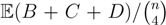 , tends to 2/3 as n → ∞ and that the variance of (B + C + D)/ tends to zero as n → ∞, when all (binary or general) trees are sampled with equal probability [6]. A further desirable feature of the quartet and triplet distances is that quartets and triplets play a fundamental role in many approaches to phylogenetic tree reconstruction (see, e.g., the R* method in Dendroscope [8] or the Quartet MaxCut method [9]).
3. Computing the Triplet and Quartet Distances between Binary Trees
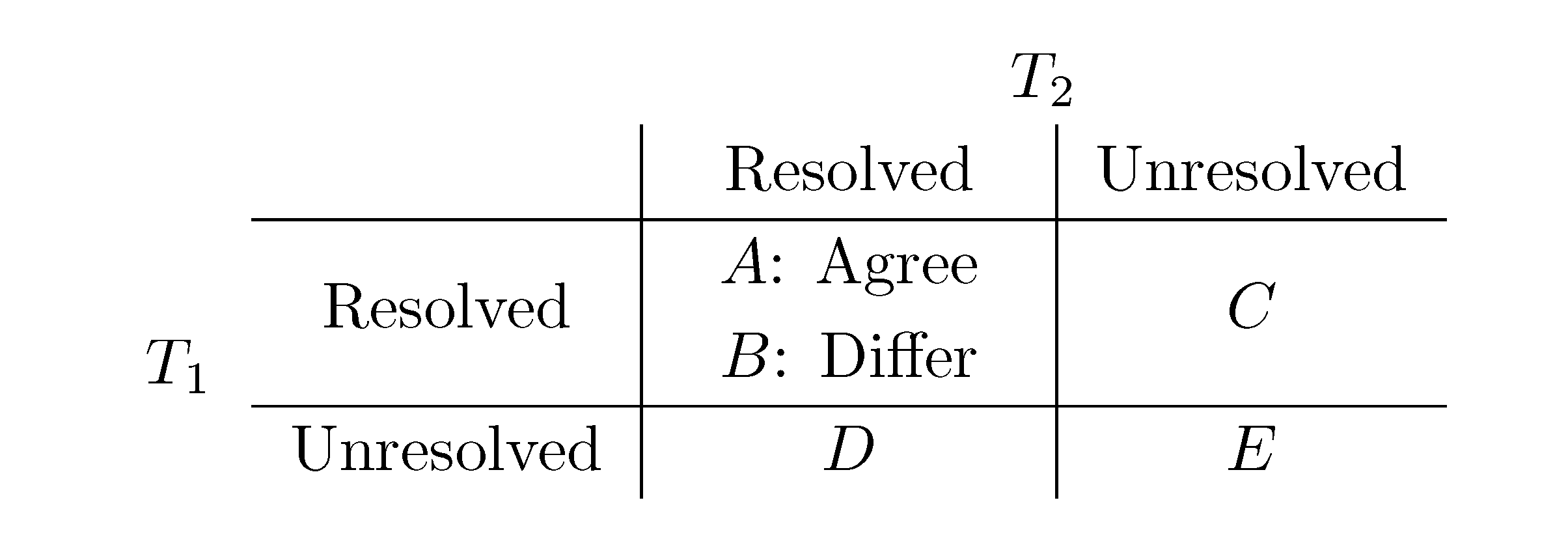
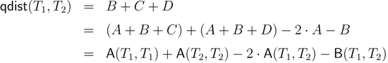
− A for the triplet distance and B = − A for the quartet distance.3.1. A Dynamic Programming Approach
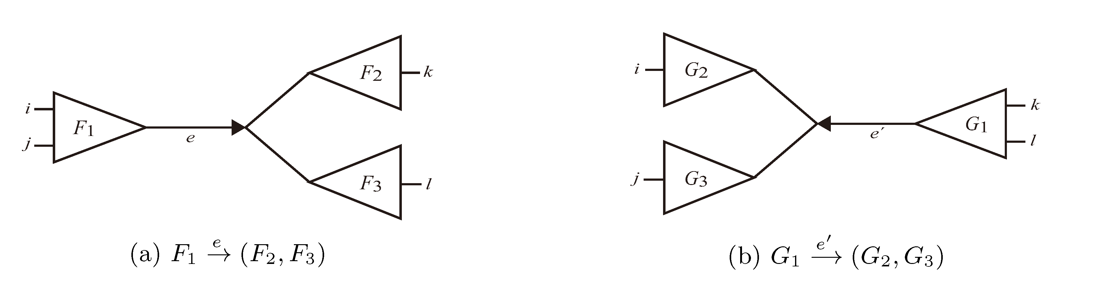
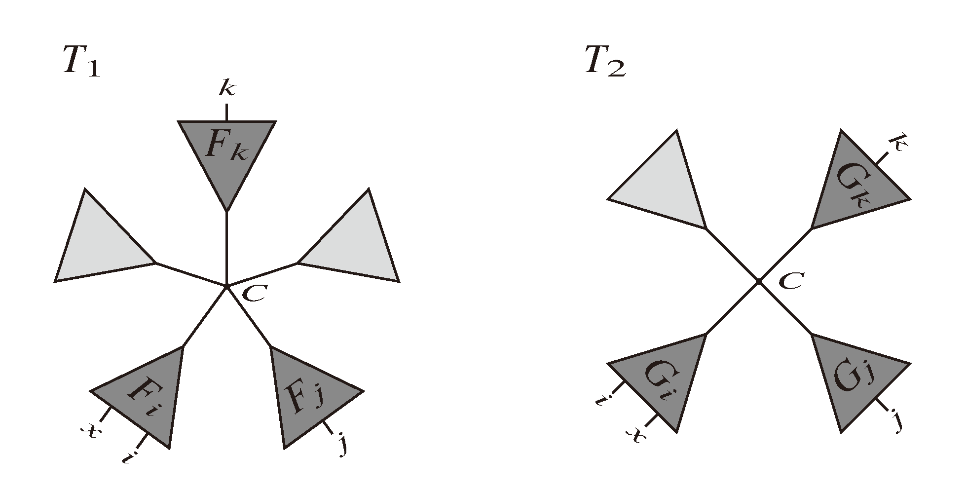
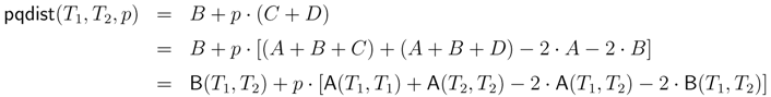
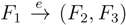 and say that the directed edge, , claims all quartets, ij|kl, with i, j ∈ F1, k ∈ F2 and l ∈ F3 (or l ∈ F2 and k ∈ F3). If a tree contains the quartet topology, ij|kl, it will be claimed by exactly two such edges: with i,j ∈ F1, k ∈ F2 and l ∈ F3 (or l ∈ F2 and k ∈ F3); and
 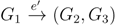 with k, l ∈ G1, i ∈ G2 and j ∈ G3 (or j ∈ G2 and i ∈ G3) as in Figure 3b.
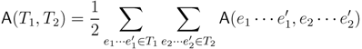
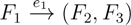 in T1 and
 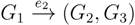 in T2, and counts how many oriented quartets, ij → kl, are claimed by both e1 and e2. This number, denoted A(e1,e2), can be computed as:

3.2. Tree Coloring
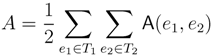
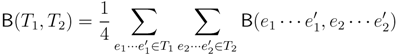
 oriented quartets, and similar to before, each quartet is associated with exactly two inner nodes. Furthermore, similar to before, the idea is to compute the double sum
 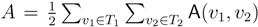 , where A(v1, v2) now denotes the number of oriented quartets (in the remainder of this section, we will use quartet and oriented quartet interchangeably) associated with nodes, v1 and v2, which induce the same quartet topology in both T1 and T2. The two algorithms, however, only explicitly iterate over the nodes in T1, while for each v1 ∈ T1, they compute
  implicitly using a data structure called the hierarchical decomposition tree of T2. To realize this strategy, both algorithms use a coloring procedure in which the leaves of the two trees are colored using the three colors,
  ,
,  and
and  . For an internal node, v1 ∈ T1, we say that T1 is colored according to v1 if the leaves in one of the subtrees all have the color, , the leaves in another of the subtrees all have the color, , and the leaves in the remaining subtree all have the color, . Additionally, we say that a quartet, ij → kl, is compatible with a coloring if i and j have different colors and k and l both have the remaining color. From this setup, we immediately get that if T1 is colored according to a node, v1 ∈ T1, then the set of quartets in T1 that are compatible with this coloring is exactly the set of quartets associated with v1 and, furthermore, if we color the leaves of T2 in the same way as in T1, that the set of quartets, S, in T2 that are compatible with this coloring is exactly the set of quartets that are associated with v1 and induce the same topology in both T1 and T2; thus, = |S|.
3.2.1. Coloring Leaves in T1 Using the “Smaller-Half Trick”
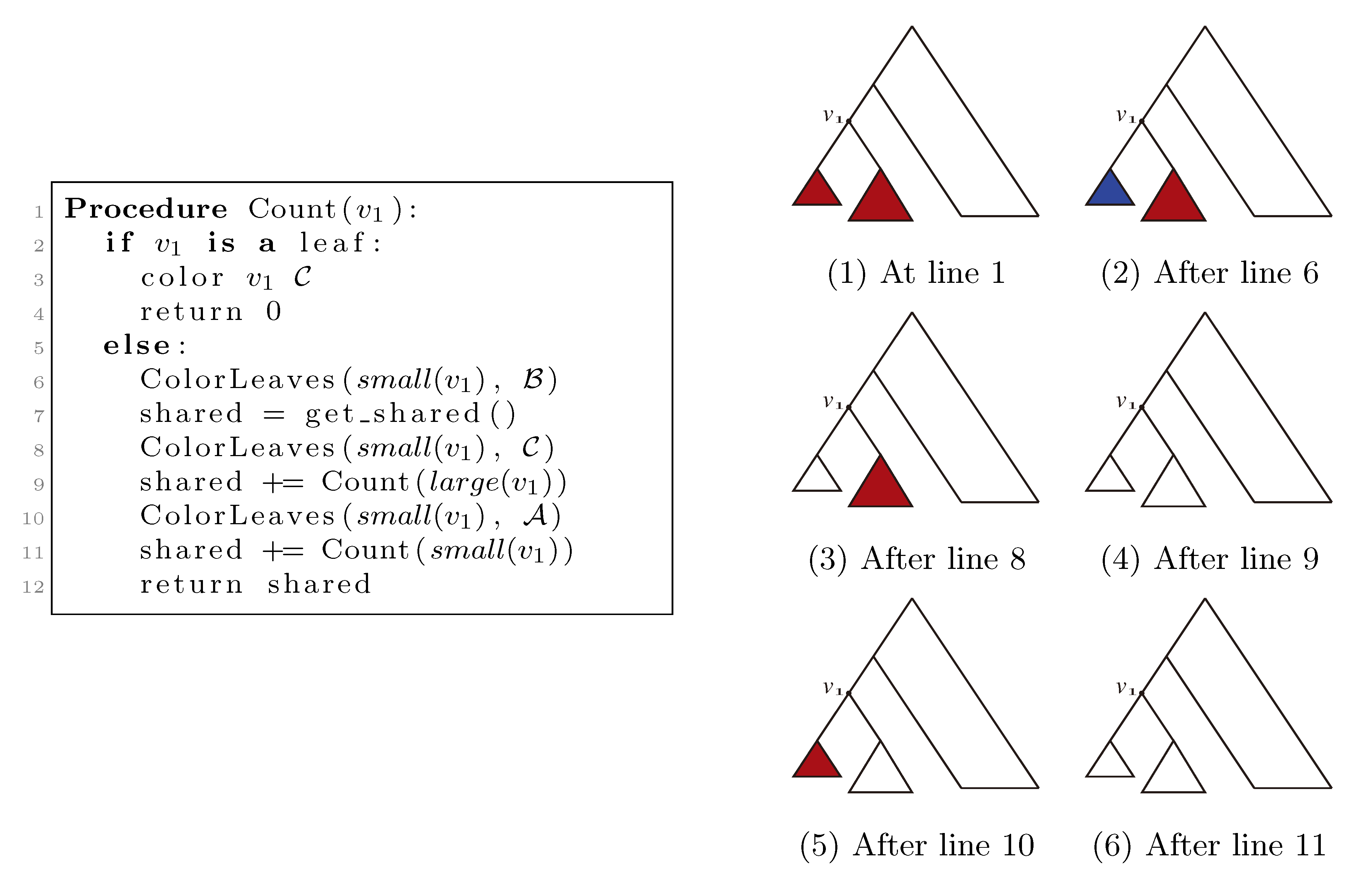
, and the new root is colored by the color, . The procedure then runs through all colorings of T1 recursively, as described and illustrated in Figure 4, starting at the single child of the root of T1. In Figure 4, large(v1), respectively small(v1), denotes the child of v1 that constitutes the root of the largest, respectively smallest, of the two subtrees under v1, measured on the number of leaves in the subtrees, and get_shared() is a call to the hierarchical decomposition of T2 to retrieve the number of quartets in T2 that are compatible with the current coloring. During the traversal, the following two invariants are maintained for all nodes, v1 ∈ T1: (1) when Count(v1) is called, all leaves in the subtree rooted at v1 have the color, , and all other leaves have the color, ; and (2) when Count(v1) returns, all leaves have the color, . As illustrated in Figure 4, these invariants imply that when get_shared() is called as a subprocedure of Count(v1), then T1 is colored according to v1. Hence, the correctness of the algorithm follows, assuming that get_shared() returns the number of oriented quartets in T2 compatible with the current coloring of the leaves.
3.2.2. The Hierarchical Decomposition Tree
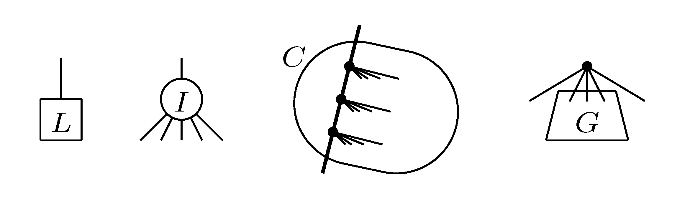
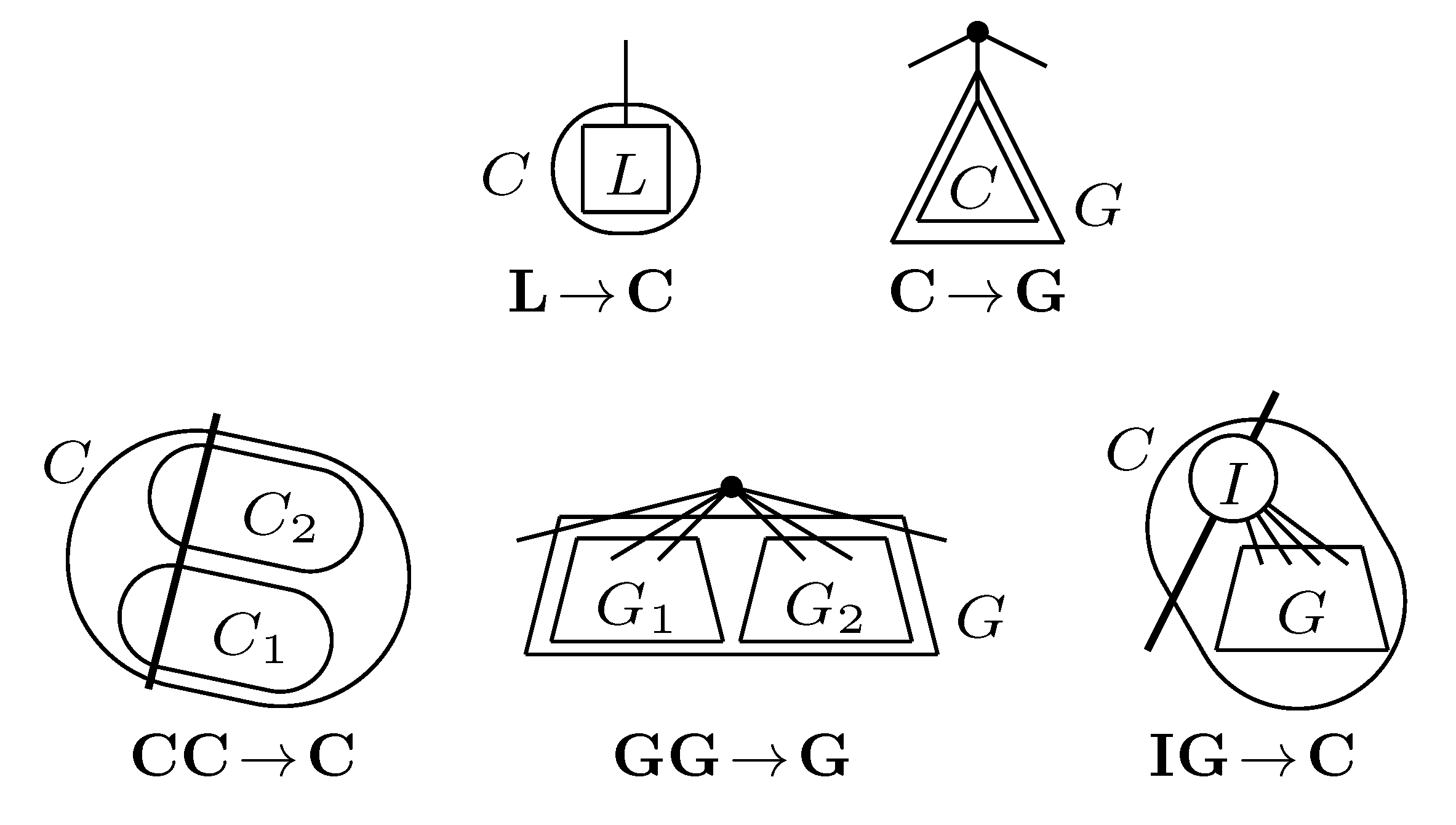
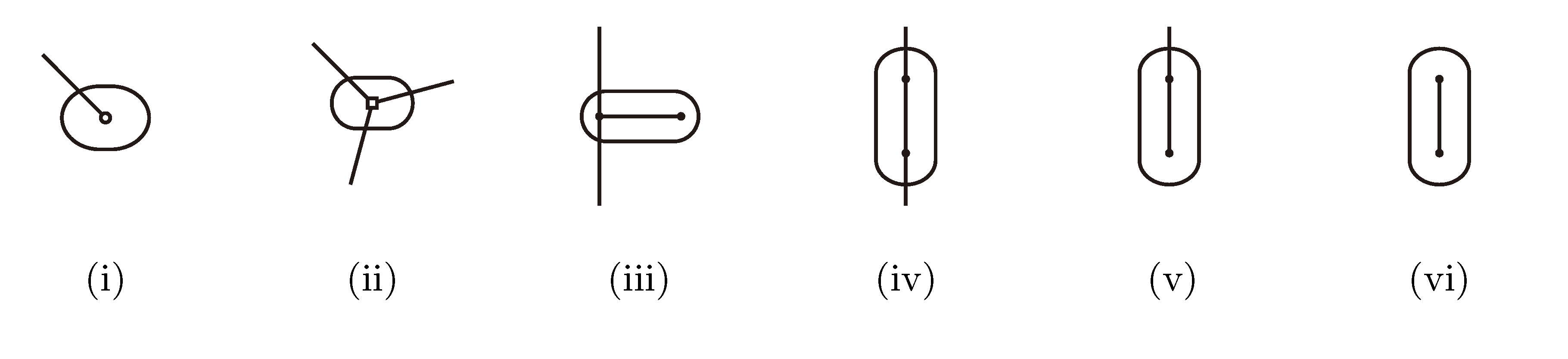 , and , respectively, in the connected component of T2 represented by C. The function F takes three parameters for each external edge of C (all components have between zero and three external edges, depending on their type, e.g., type (i) components have one external edge, while type (iii) components have two). If C has k external edges, we number these arbitrarily from one to k and denote the three parameters for edge i by ai, bi and ci. Of the two ends of an external edge, one is in the component and the other is not. The parameters, ai, bi and ci, denote the number of leaves with colors , and , respectively, which are in the subtree of T2 rooted at the endpoint of edge i that is not in C. Finally, F states, as a function of these parameters, the number of elements of the quartets, which are both associated with nodes contained in C and compatible with the current coloring of the leaves. It turns out that F is a polynomial of a total degree of at most four.
3.2.3. Tweaking the Algorithm to Obtain Time Complexity O(n log n)
 for each inner node v and cv = 0 for each leaf v, then we have a total cost of Σv∈T cv ≤ n log n. This means that if we can decrease the time used per inner node v1 in T1 from |small(v1)| log n, as in the previous two subsections, to
  , the total time used will be reduced from O(n log2 n) to O(n log n).
 , we first observe that a hierarchical decomposition tree is a locally-balanced binary rooted tree. A binary rooted tree is c-locally-balanced if for all nodes v in the tree, the height of the subtree rooted at v is at most c(1 + log |v|). To be exact, our hierarchical decomposition trees are
  -locally-balanced (see [15] for the proof of this). A locally-balanced tree with n nodes has the property that the union of k different leaf-to-root paths contains just
  nodes (see Lemma 4 in [15]). Thus, since each v1 ∈ T1 HDT(T2(v1)) has O(|v1|) nodes, the |small(v1)| leaf-to-root paths in HDT(T2(v)) that need to be updated when visiting v1 contain nodes in total. This means that if we spend only constant time to update each of these, we get a total time for coloring and counting, still disregarding the time used to build contractions, of O(n log n) by the extended smaller-half trick. To spend only constant time for each of the nodes, we split the update procedure for HDT(T2(v1)) after the |small(v1)| color changes in two in the following way: (1) We first mark all internal nodes in HDT(T2(v1)) on paths from the |small(v1)| type (i) components to the root by marking bottom-up from each of the type (i) components, until we find the first already marked component. (2) We then update all the marked nodes recursively in a postorder traversal starting at the root of HDT(T2(v1))., and we will not do it from scratch every time. Figure 6 shows how this is achieved using the subroutines, Contract and Extract. In this pseudo-code, T2 and are used to refer to the tree, T2, as well as their associated hierarchical decomposition trees.
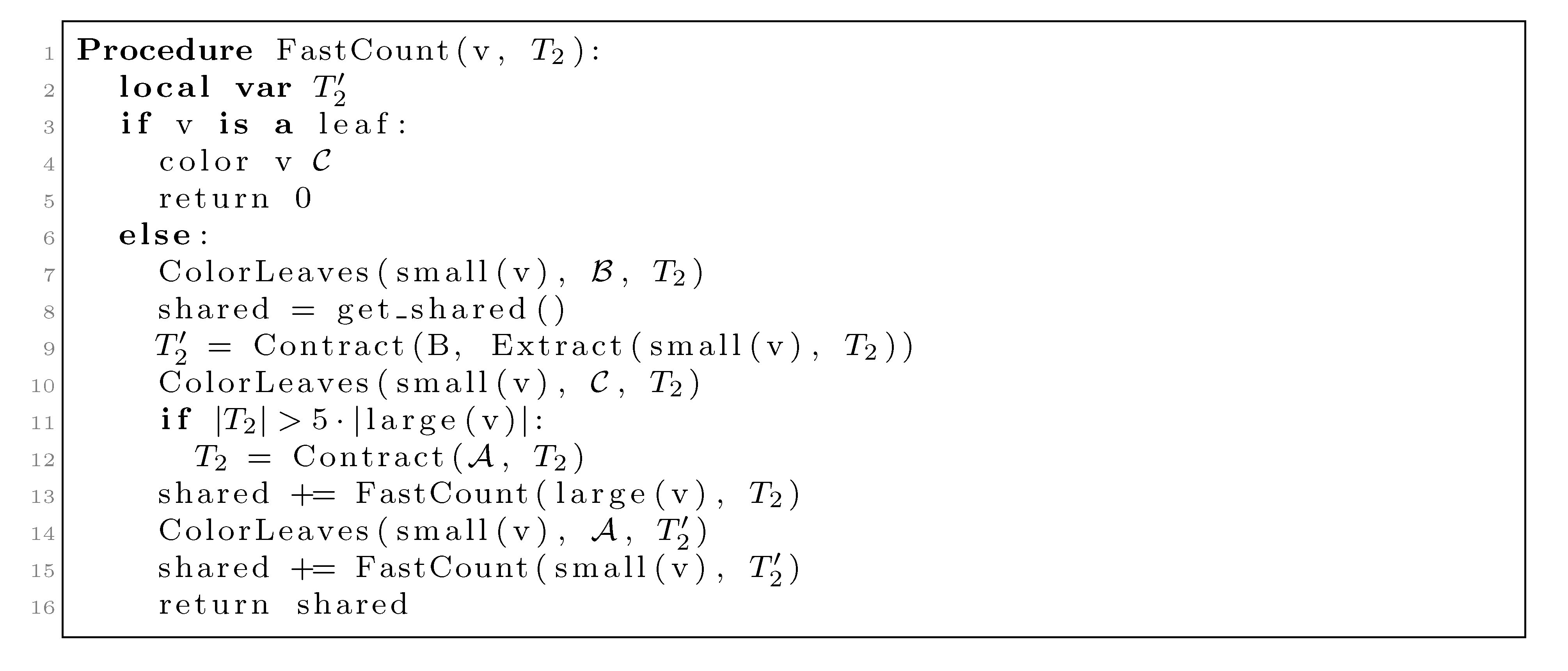 , but all other leaves have the color . The first call to Contract in line 9 builds a contraction, , of this copy, and this contraction is used as T2 in the recursive call on small(v1) in line 15. The second call to Contract in line 12 is only executed when |T2| > 5|large(v1)| (i.e., when more than 4/5 of the leaves have the color, ). This contraction is used in the recursive call on large(v1) in line 13.
 (see [15]); thus, since |T2| = |v1| when we perform it, the total time used on this line is O(n log n) by the extended smaller-half trick. We now consider the time spent on contracting T2 in line 12. We perform this line whenever |T2| > 5|large(v1)|. Since all leaves in large(v1) are colored when we contract, the size of the new T2 has at most 4|large(v1)| − 5 nodes. Hence, the size of T2 is reduced by a factor of 4/5. This implies that the sequence of contractions applied to a hierarchical decomposition results in a sequence of data structures of geometrically decaying sizes. Since a contraction takes time O(|T2|), the total time spent on line 12 is linear in the initial size of T2, i.e., it is dominated by the time for constructing the initial hierarchical decomposition tree, which is O(n). In total, we therefore use O(n log n) time for contracting and extracting T2.
4. Dealing with General Trees
4.1. Dynamic Programming Approaches

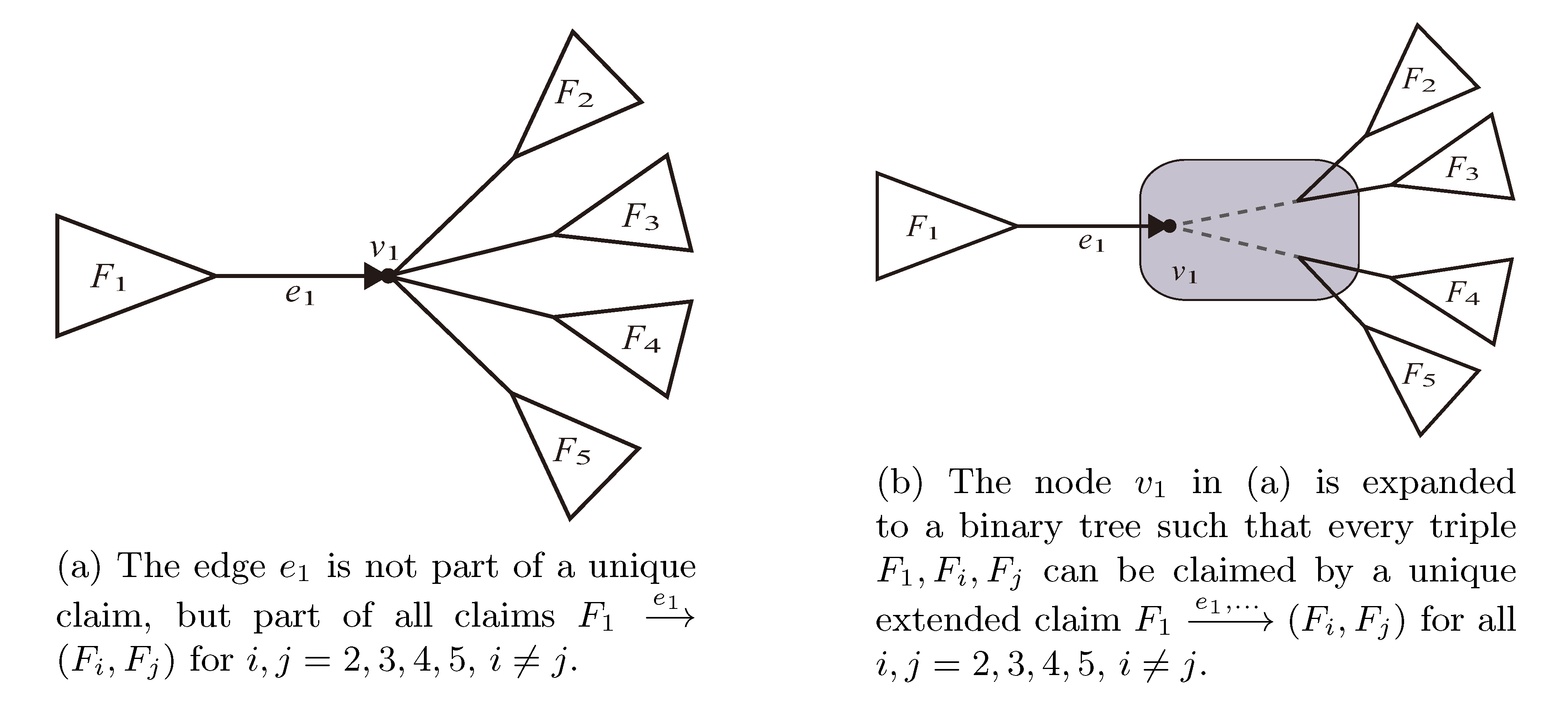
 , and the quartets they claim. Consider oriented edges e1 and e2 in T1 and T2, respectively, and let v1 and v2 denote the destination nodes of the edges. If v1 or v2 are high-degree nodes, then the edges do not correspond to unique claims, and , since the trees, F2, F3, G2 and G3, are not uniquely defined (see Figure 9a). To get around this, the algorithm transforms the trees by expanding (arbitrarily) each high-degree node into a binary tree, tagging edges, so we can distinguish between original edges and edges caused by the expansion (see Figure 9b). We then define extended claims,
  , consisting of two edges, e1 and , such that e1 is one of the original edges, is a result of expanding nodes and such that the oriented path from e1 to only goes through expansion edges. The extended claims play the role that claims do in the original algorithm, and each resolved quartet in the original tree is claimed by exactly two extended claims in the expanded tree.

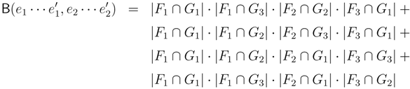
 claims ij → kl (i.e., i, j ∈ F1, k ∈ F2 and l ∈ F3) and
 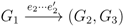 claims ik → jl, il → jk, jk → il or jl → ik, we can count as:
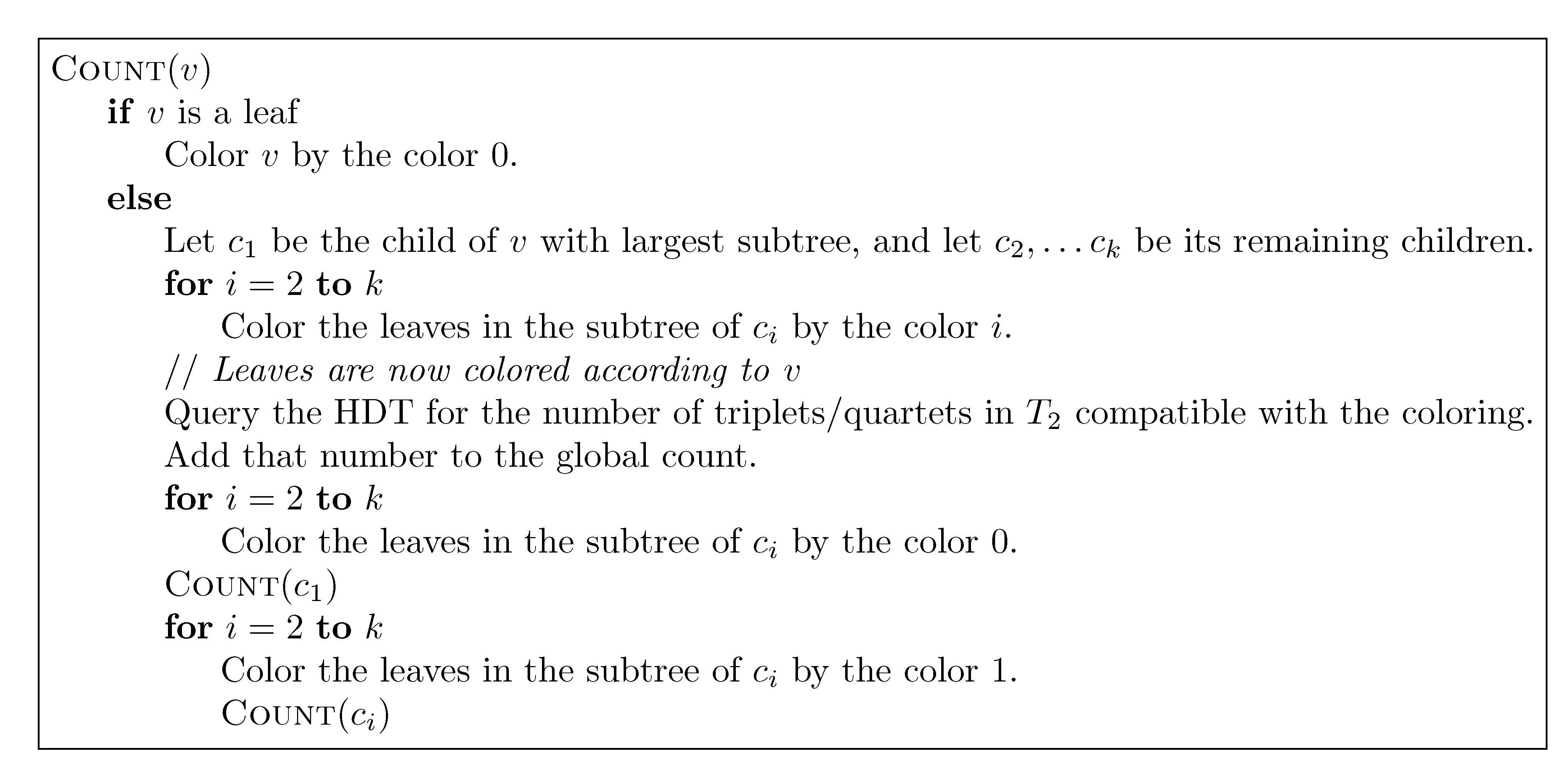
4.2. Tree Coloring


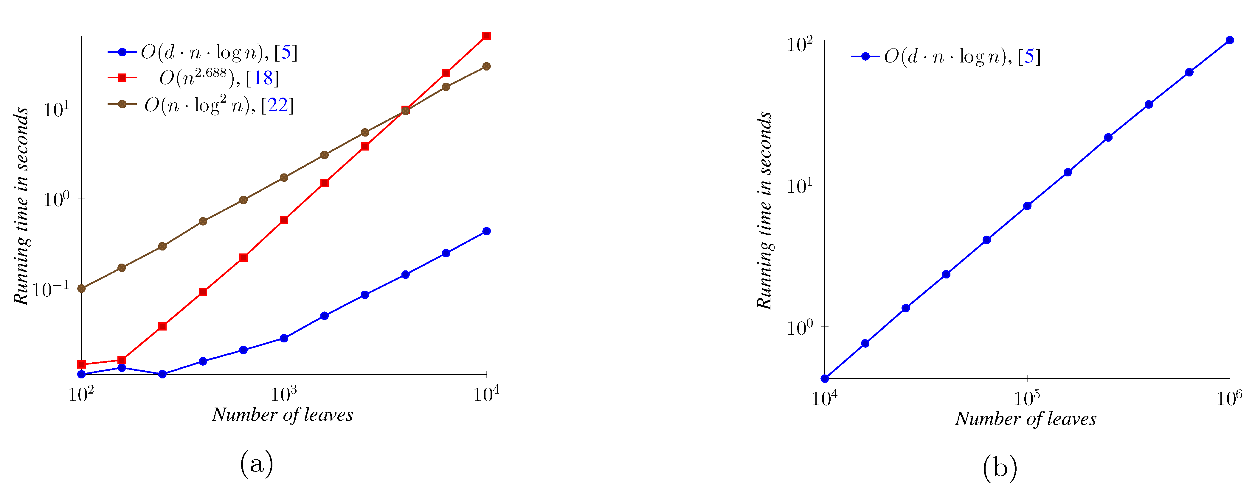
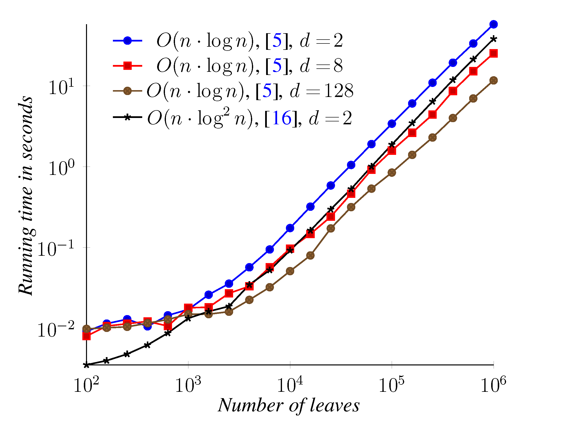
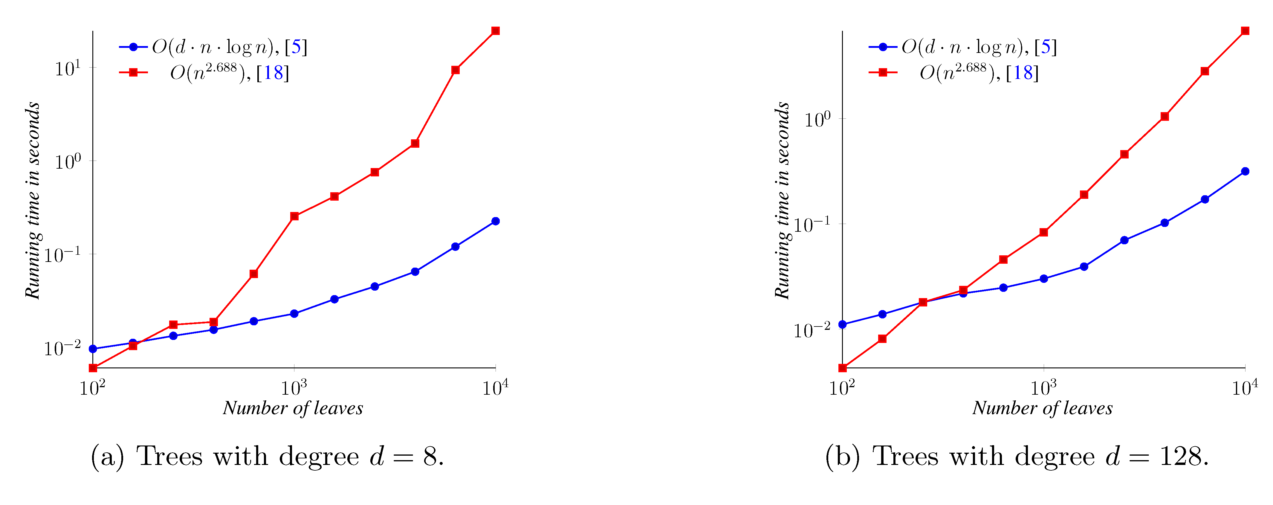
5. Experimental Results


6. Conclusions
Acknowledgments
References
- Robinson, D.; Foulds, L.R. Comparison of phylogenetic trees. Math. Biosci. 1981, 53, 131–147. [Google Scholar] [CrossRef]
- Estabrook, G.F.; McMorris, F.R.; Meacham, C.A. Comparison of undirected phylogenetic trees based on subtrees of four evolutionary units. Syst. Zool. 1985, 34, 193–200. [Google Scholar] [CrossRef]
- Critchlow, D.E.; Pearl, D.K.; Qian, C. The triples distance for rooted bifurcating phylogenetic trees. Syst. Biol. 1996, 45, 323–334. [Google Scholar] [CrossRef]
- Day, W.H.E. Optimal-algorithms for comparing trees with labeled leaves. J. Classif. 1985, 2, 7–28. [Google Scholar] [CrossRef]
- Brodal, G.S.; Fagerberg, R.; Mailund, T.; Pedersen, C.N.S.; Sand, A. Efficient Algorithms for Computing the Triplet and Quartet Distance between Trees of Arbitrary Degree. In Proceedings of the annual ACM-SIAM Symposium on Discrete Algorithms (SODA), New Orleans, LA, USA, January 2013; pp. 1814–1832.
- Steel, M.; Penny, D. Distributions of tree comparison metrics—Some new results. Syst. Biol. 1993, 42, 126–141. [Google Scholar]
- Bandelt, H.J.; Dress, A. Reconstructing the shape of a tree from observed dissimilarity data. Adv. Appl. Math. 1986, 7, 309–343. [Google Scholar] [CrossRef]
- Huson, D.H.; Scornavacca, C. Dendroscope 3: An interactive tool for rooted phylogenetic trees and networks. Syst. Biol. 2012, 61, 1061–1067. [Google Scholar] [CrossRef]
- Snir, S.; Rao, S. Quartet MaxCut: A fast algorithm for amalgamating quartet trees. Mol. Phylogenetics Evol. 2012, 62, 1–8. [Google Scholar] [CrossRef]
- Bansal, M.S.; Dong, J.; Fernández-Baca, D. Comparing and aggregating partially resolved trees. Theor. Comput. Sci. 2011, 412, 6634–6652. [Google Scholar] [CrossRef]
- Pompei, S.; Loreto, V.; Tria, F. On the accuracy of language trees. PLoS One 2011, 6, e20109. [Google Scholar] [CrossRef]
- Walker, R.S.; Wichmann, S.; Mailund, T.; Atkisson, C.J. Cultural phylogenetics of the Tupi language family in lowland South America. PLoS One 2011, 7, e35025. [Google Scholar]
- Bryant, D.; Tsang, J.; Kearney, P.; Li, M. Computing the Quartet Distance between Evolutionary Trees. In Proceedings of the annual ACM-SIAM Symposium on Discrete Algorithms, San Francisco, CA, USA, January 2000.
- Brodal, G.S.; Fagerberg, R.; Pedersen, C.N.S. Computing the Quartet Distance Between Evolutionary Trees in Time O(n log2 n). In Proceedings of the annual International Symposium on Algorithms and Computation, Christchurch, New Zealand, 19–21 December; Springer: Berlin/ Heidelberg, Germany, 2001; Volume 2223, pp. 731–742. [Google Scholar]
- Brodal, G.S.; Fagerberg, R.; Pedersen, C.N.S. Computing the quartet distance between evolutionary trees in time O(n log n). Algorithmica 2004, 38, 377–395. [Google Scholar] [CrossRef]
- Sand, A.; Brodal, G.S.; Fagerberg, R.; Pedersen, C.N.S.; Mailund, T. A practical O(n log2 n) time algorithm for computing the triplet distance on binary trees. BMC Bioinforma. 2013, 14, S18. [Google Scholar]
- Mehlhorn, K. Data Structures and Algorithms: Sorting and Searching; Springer: Berlin/ Heidelberg, Germany, 1984. [Google Scholar]
- Buneman, O.P. The recovery of trees from measures of dissimilarity. In Mathematics of the Archeological and Historical Sciences; Kendall, D.G., Tautu, P., Eds.; Columbia University Press: New York, NY, USA, 1971; pp. 387–395. [Google Scholar]
- Bryant, D.; Moulton, V. A polynomial time algorithm for constructing the refined buneman tree. Appl. Math. Lett. 1999, 12, 51–56. [Google Scholar] [CrossRef]
- Christiansen, C.; Mailund, T.; Pedersen, C.N.S.; Randers, M. Computing the Quartet Distance Between Trees of Arbitrary Degree. In Proceeding of the annual Workshop on Algorithms in Bioinformatics, Mallorca, Spain, 3–6 October 2005; Springer: Berlin/Heidelberg, Germany, 2005; Volume 3692, pp. 77–88. [Google Scholar]
- Christiansen, C.; Mailund, T.; Pedersen, C.N.S.; Randers, M.; Stissing, M. Fast calculation of the quartet distance between trees of arbitrary degrees. Algorithms Mol. Biol. 2006, 1, 16–16. [Google Scholar] [CrossRef]
- Nielsen, J.; Kristensen, A.; Mailund, T.; Pedersen, C.N.S. A sub-cubic time algorithm for computing the quartet distance between two general trees. Algorithms Mol. Biol. 2011. [Google Scholar] [CrossRef]
- Coppersmith, D.; Winograd, S. Matrix multiplication via arithmetic progressions. J. Symb. Comput. 1990, 9, 251–280. [Google Scholar] [CrossRef]
- Stissing, M.; Pedersen, C.N.S.; Mailund, T.; Brodal, G.S.; Fagerberg, R. Computing the Quartet Distance between Evolutionary Trees of Bounded Degree. In Proceedings of the Asia-Pacific Bioinformatics Conference, Hong Kong, 15–17 January 2007; pp. 101–110.
- Johansen, J.; Holt, M.K. Computing Triplet and Quartet Distances. Master’s Thesis, Aarhus University, Department of Computer Science, Aarhus, Denmark, 2013. [Google Scholar]
- Mailund, T.; Pedersen, C.N.S. QDist–Quartet distance between evolutionary trees. Bioinformatics 2004, 20, 1636–1637. [Google Scholar] [CrossRef]
© 2013 by the authors; licensee MDPI, Basel, Switzerland. This article is an open access article distributed under the terms and conditions of the Creative Commons Attribution license (http://creativecommons.org/licenses/by/3.0/).
Share and Cite
Sand, A.; Holt, M.K.; Johansen, J.; Fagerberg, R.; Brodal, G.S.; Pedersen, C.N.S.; Mailund, T. Algorithms for Computing the Triplet and Quartet Distances for Binary and General Trees. Biology 2013, 2, 1189-1209. https://doi.org/10.3390/biology2041189
Sand A, Holt MK, Johansen J, Fagerberg R, Brodal GS, Pedersen CNS, Mailund T. Algorithms for Computing the Triplet and Quartet Distances for Binary and General Trees. Biology. 2013; 2(4):1189-1209. https://doi.org/10.3390/biology2041189
Chicago/Turabian StyleSand, Andreas, Morten K. Holt, Jens Johansen, Rolf Fagerberg, Gerth Stølting Brodal, Christian N. S. Pedersen, and Thomas Mailund. 2013. "Algorithms for Computing the Triplet and Quartet Distances for Binary and General Trees" Biology 2, no. 4: 1189-1209. https://doi.org/10.3390/biology2041189
APA StyleSand, A., Holt, M. K., Johansen, J., Fagerberg, R., Brodal, G. S., Pedersen, C. N. S., & Mailund, T. (2013). Algorithms for Computing the Triplet and Quartet Distances for Binary and General Trees. Biology, 2(4), 1189-1209. https://doi.org/10.3390/biology2041189