Label Self-Advised Support Vector Machine (LSA-SVM)—Automated Classification of Foot Drop Rehabilitation Case Study

 , and
, and 
Abstract
:1. Introduction
2. Related Work
2.1. The Standard SVM
2.2. Self-Advised Support Vector Machine (SA-SVM)
- Classify the hyper-plane founded by applying the decision function is Equation (4):
- Misclassified data that samples in the first train phase are recognized. The misclassified datasets (MD) in the training phase are calculated by Equation (5):The MD set may be null but the empirical outcomes appear when the presence of misclassified data in the training phase is a communal existence. It should be recognized that trying any technique to benefit from misclassified data should have a control to affect the outlier data. When the misclassified data is included to resemble samples, the use of misclassified data improved the classification accuracy [14].
- The algorithm indicates: If MD is null then go to the testing phase or else compute neighborhood length (NL) for each Xi of MD. Equation (6), defined NL.where is the training data that does not belong to the MD set. If the training data is a map with a higher dimension, the distance between xi and xj can be evaluated in Equation (7) with reference to the related RBF kernel
- Calculating Advised Weight for each sample from the test set using Equation (8). These represent the closest test data to the misclassified data.
- The absolute value of the SVM decision values for each from the test set are considered and scaled in to [0, 1].
- Finally, for each xk from the test set in Equation (9):If decision value then:which is identified with normal SVM, otherwise:
2.3. Label Classification
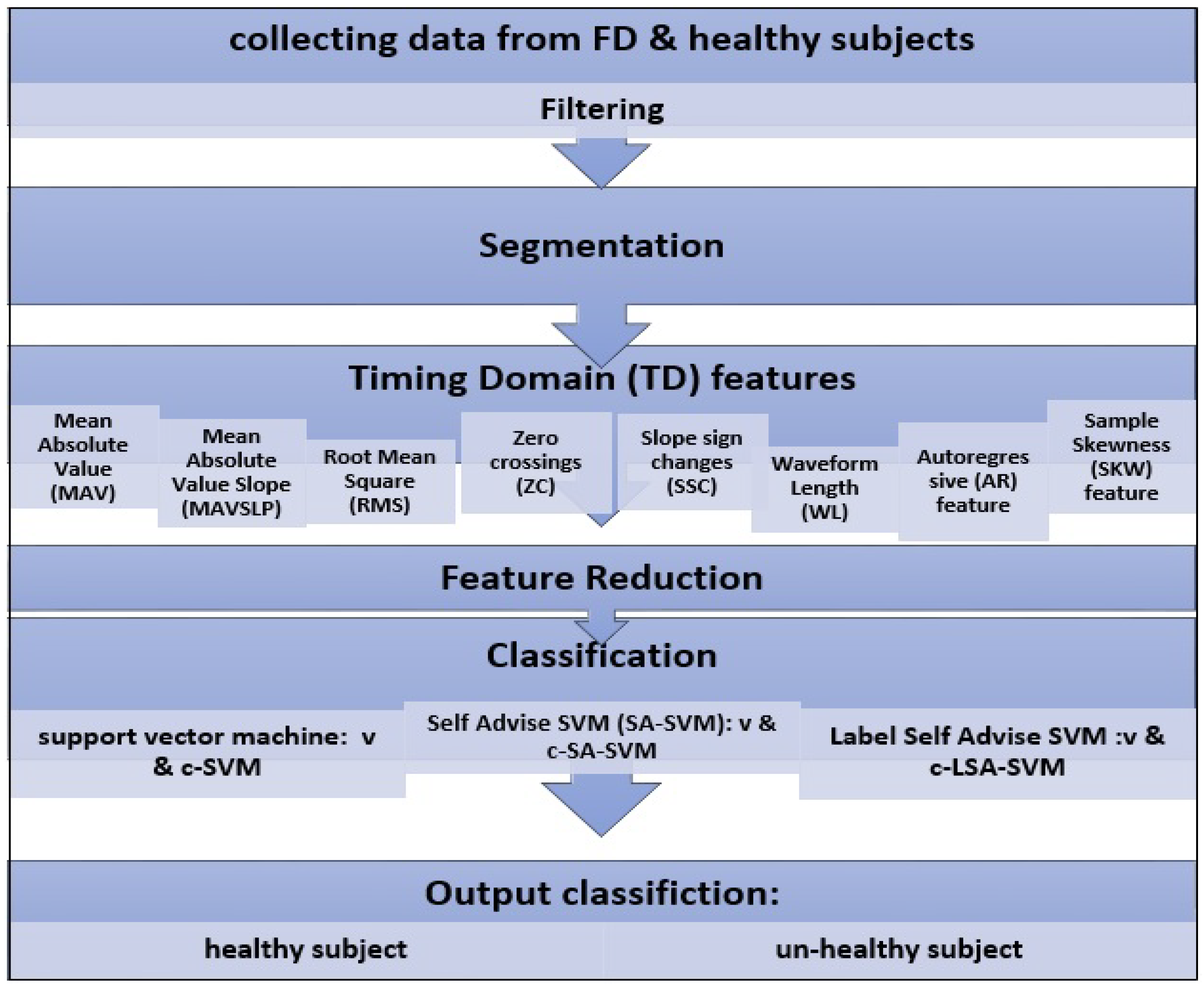
3. Materials and Methods
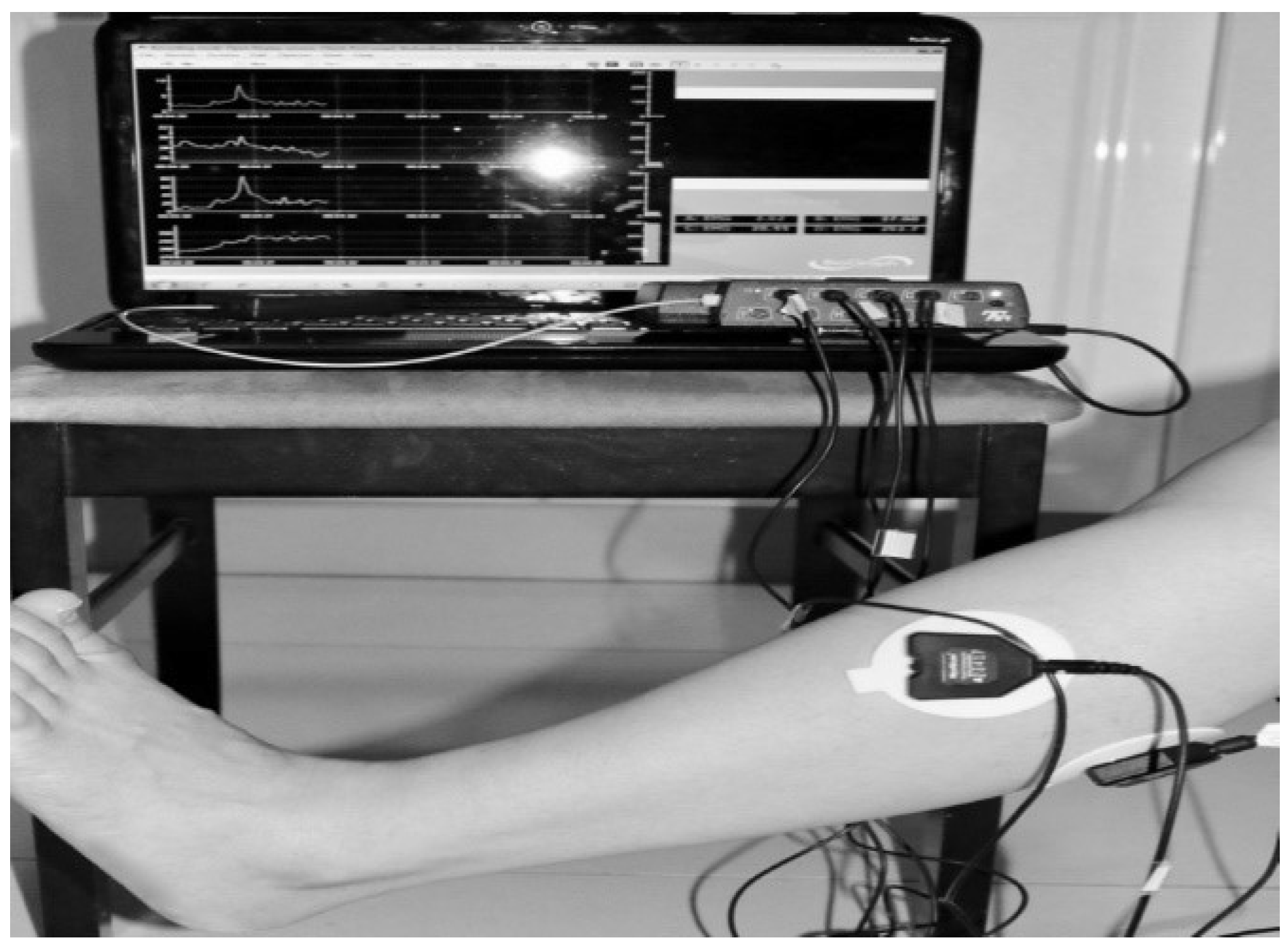
3.1. Materials
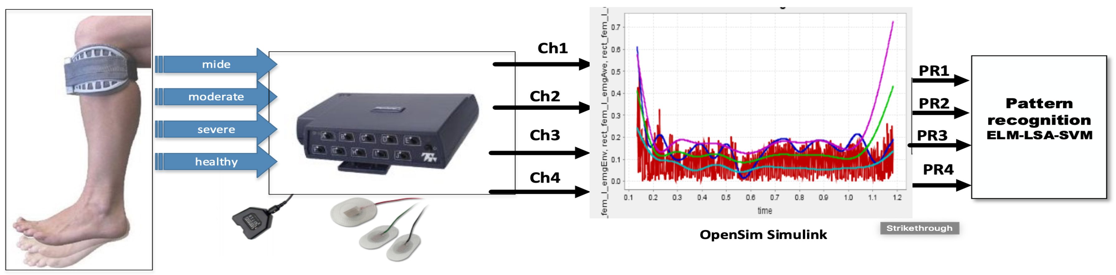
3.2. Procedure for Collecting sEMG Signal Data
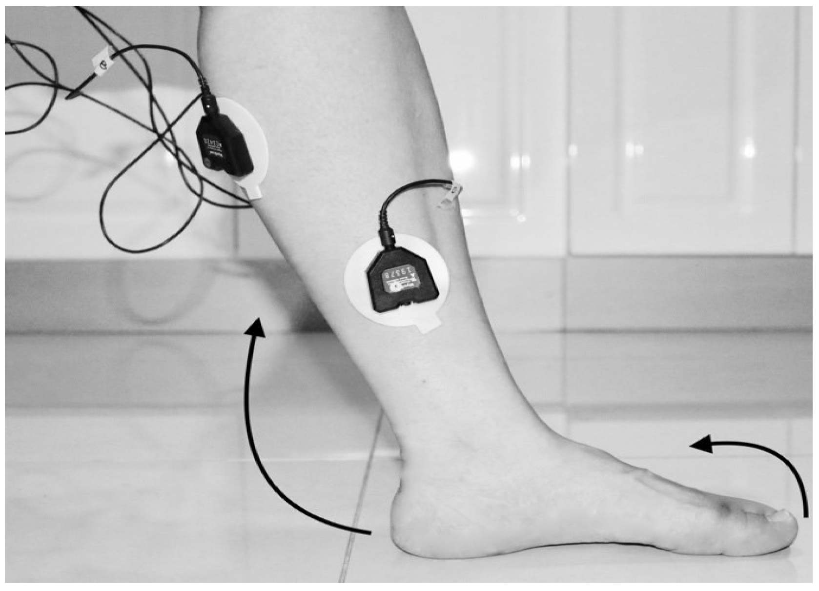
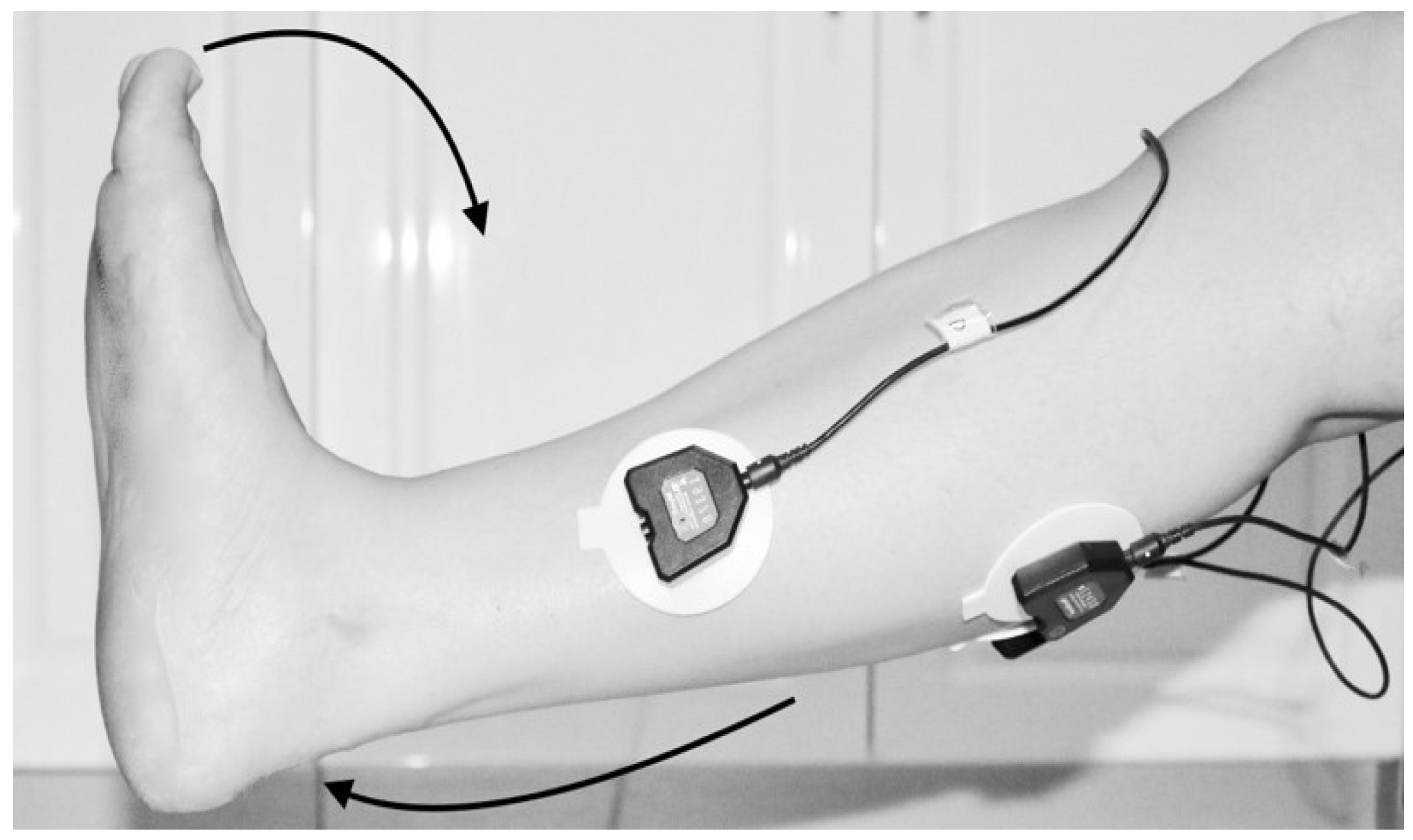
- First trial: To move (with help, if required) his/her lower limb at the knee joint. Flexion and extension (bend and straighten) from the actual position while sitting on a chair. Each set of trials took 3 s and a 5 s rest was given between two trials (two sets of trials were done for this case) as shown in Figure 4 and Figure 5.
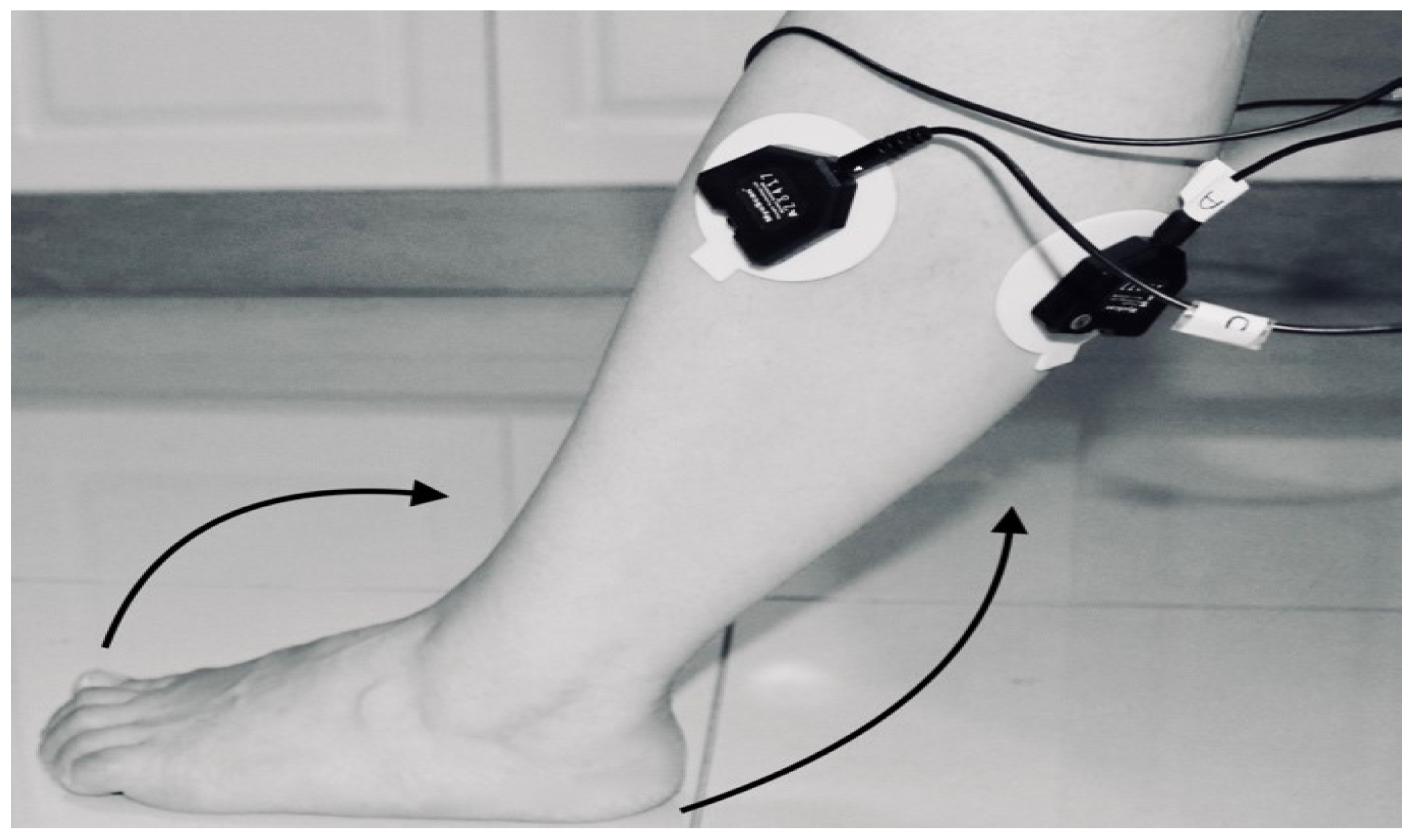
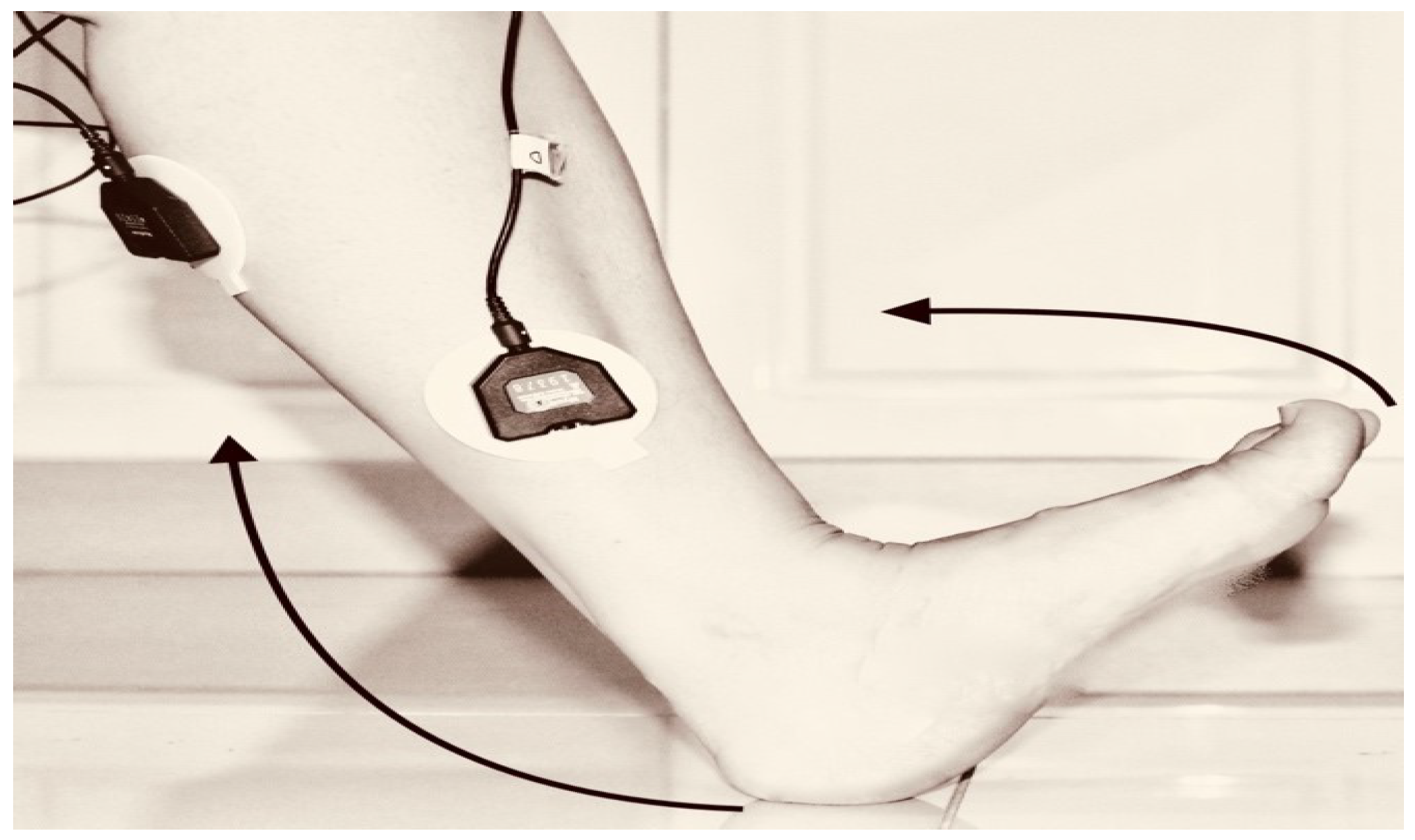
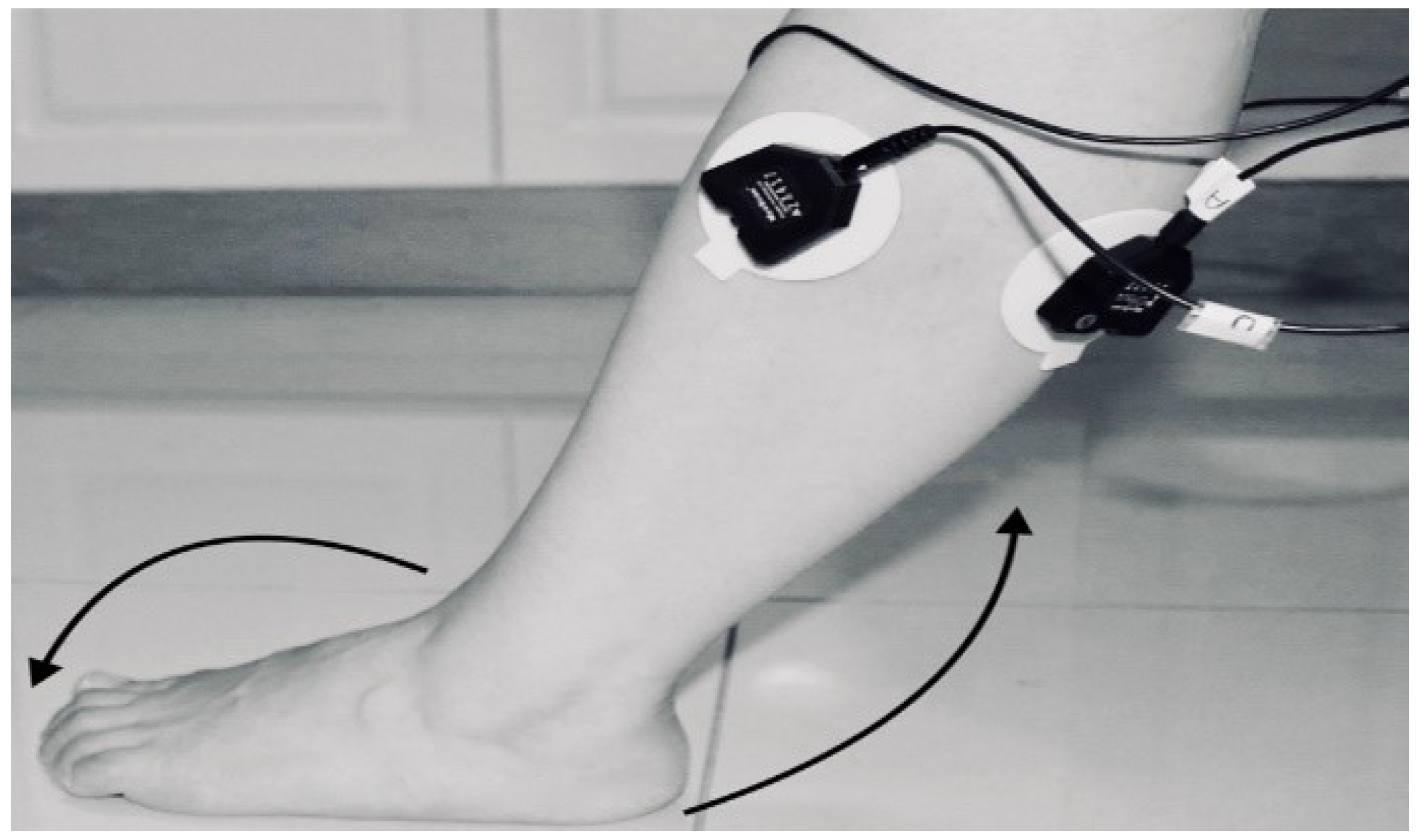
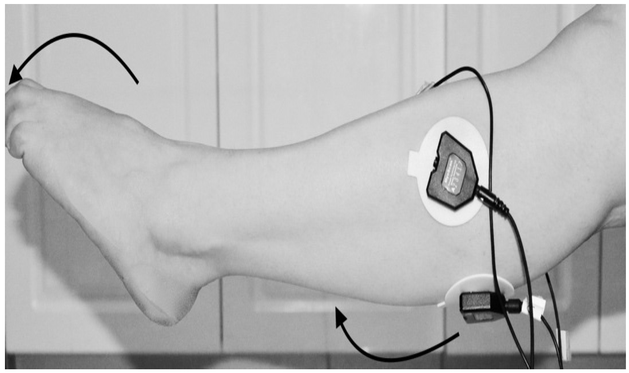
- Third trial: To move (with help, if required) his/her lower limb (foot and leg) at the knee joint, to flex or extend (bend and straighten) with Extension Plantar flexion and Flexion Dorsiflexion from the rest position while sitting on the chair. Each set of trials took 3 s and a 5 s rest was given between two trials. (Two sets of trials were done for this case) as shown in Figure 8 and Figure 9.
3.3. Method: Label Self-Advised Support Vector Machine (LSA-SVM)
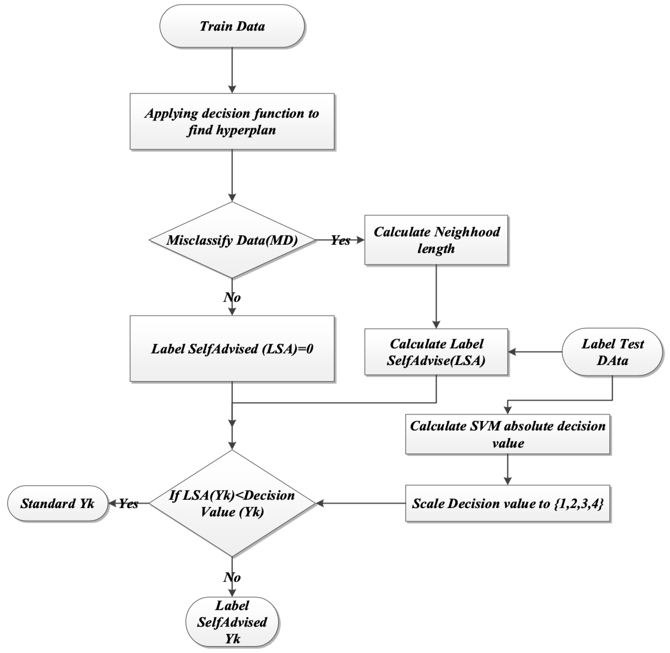
- Applying the decision function as in Equation (10), to classify hyperplane:where is the input vector for sample labeled with related to its class, while is the non-negative Lagrange multiplier, which conflicts with standard SVM training.
- Misclassified data samples in the first train phase are recognized. The misclassified data sets (MD) in the training phase are calculated by Equation (11):
- The algorithm indicates that: If MD is empty, then go to the testing phase, or else calculate neighborhood length (NL) for each yi of label MD. Equation (12) defined NL.where is the label of training data that do not belong to the label of MD set. The label of the training data is mapped to a higher dimension, the distance between and is computed according to the following Equations (13) and (14) with reference to the related RBF kernel.that is, RBF will be:
- For each label from test data, the Lab Advised Weight LAW () figures out as Equation (15). These LAWs represent how close the label test data are to the label of misclassified data.The absolute value of the SVM decision values for each xk from the test set is calculated and scaled to .
- For each from the label of the test set,If decision value then which is compatible with normal SVM labeling, otherwise . Figure 11, explain the flow chart for the steps above.
4. Experiments and Results
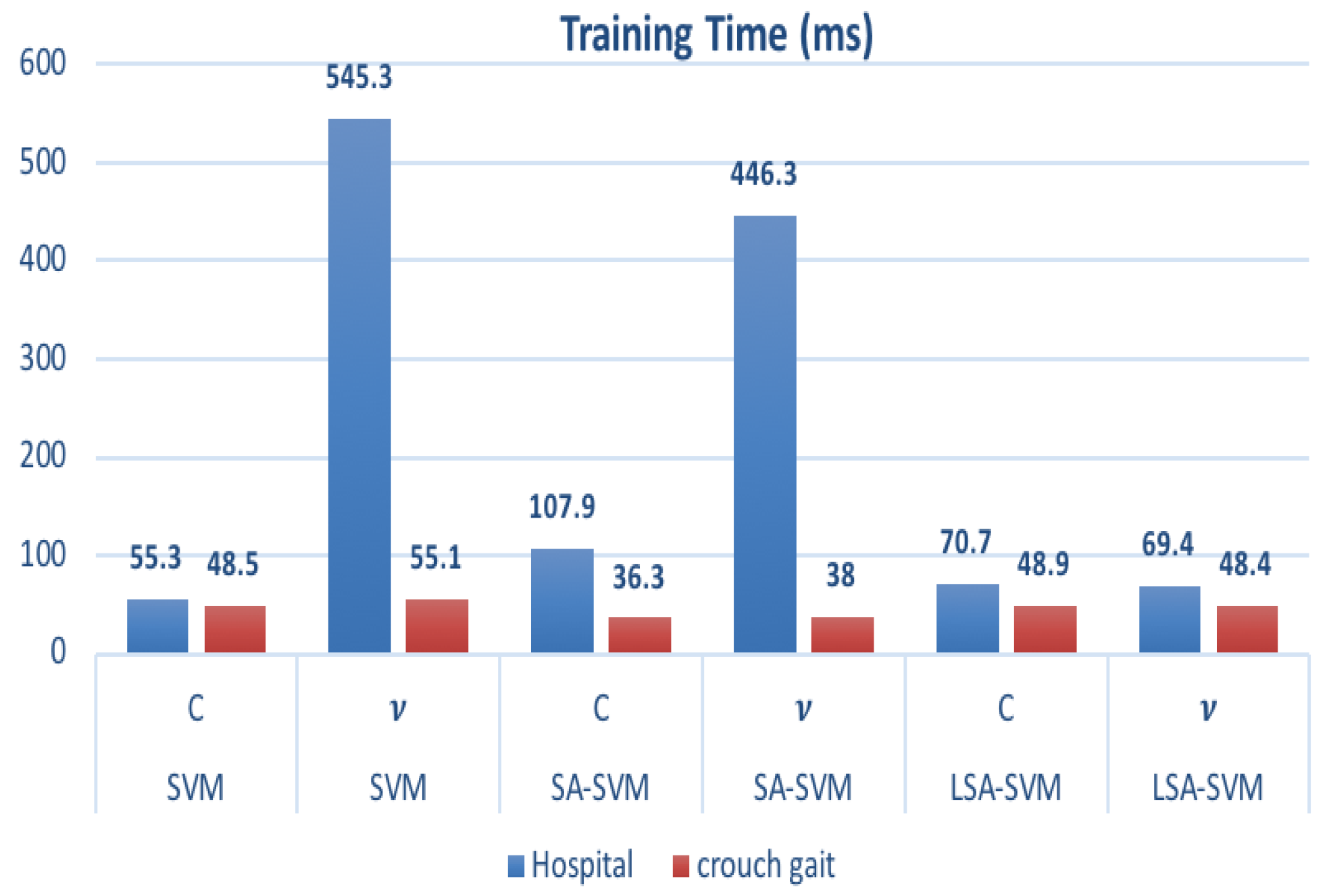
4.1. Experiments on Hospital Datasets
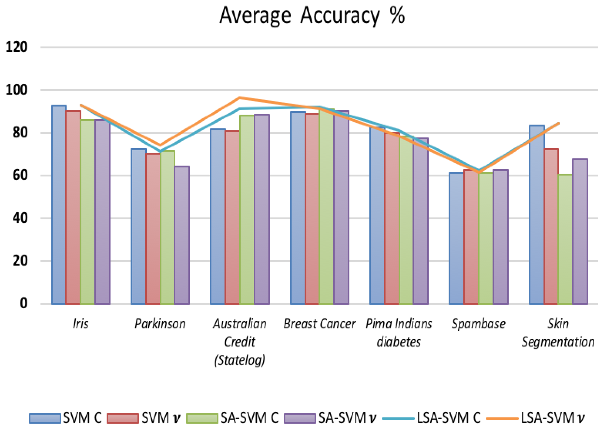
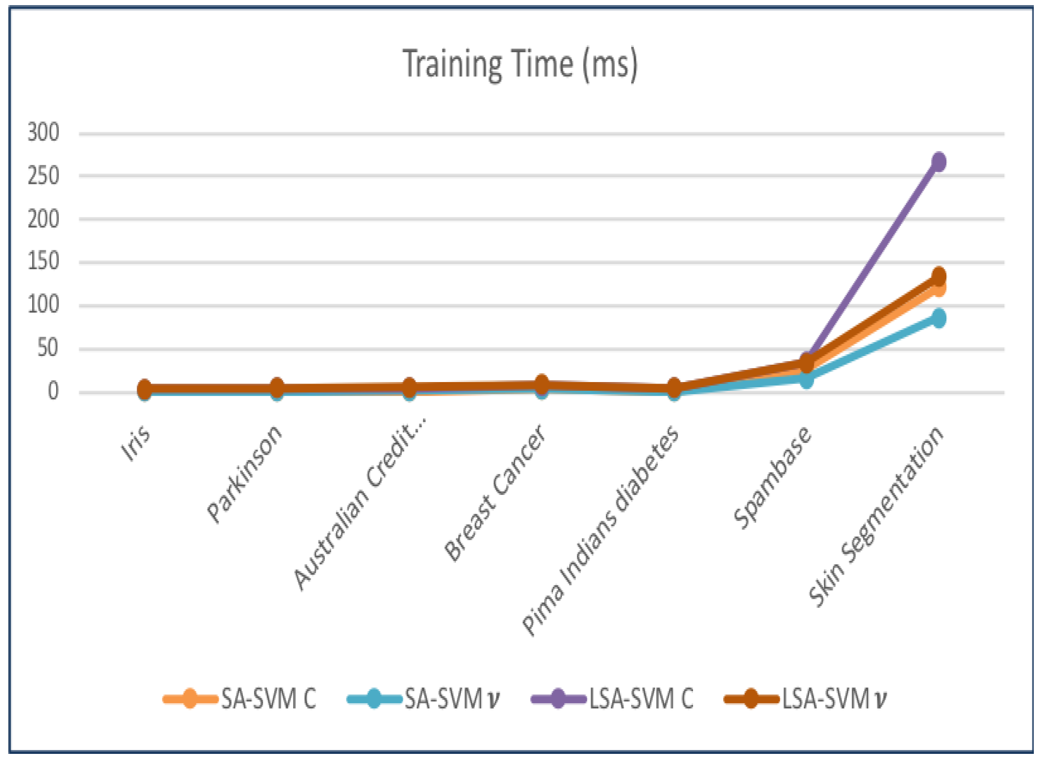
4.2. Experiments on UCI Datasets
5. Conclusions
Author Contributions
Funding
Conflicts of Interest
Abbreviations
| LAW | Lab Advised Weight |
| AW | Advised Weight |
| SVM | Support Vector Machine |
| FD | Foot drop |
| SA-SVM | Self Advised Support Vector Machine |
| LMN | Lower Motor Neuron |
| FES | Function Electrical Stimulation |
| M-PR | Myoelectric Pattern Recognition |
| SA-SVM | Self-Advised-Support Vector Machine |
| LSA-SVM | Label Self-Advised-Support Vector Machine |
| LCM | label classification methods |
| RBF | Radial Basis Function |
| MD | Misclassify Datasets |
| EMG | Electromyography |
| sEMG | surface EMG |
| TA | Tibias Anterior |
| RF | Rectus Femurs |
| Gas | Gastrocnemius |
| Sol | Soule |
| TA | Tibias Anterior |
| CG | Crouch Gait |
| LDA | Linear discriminant analysis |
| TD-AR | Timing Domain-Autoregressive |
| SCC | single class classification |
| SLC | Single Label Classification |
| MDPI | Multidisciplinary Digital Publishing Institute |
| DOAJ | Directory of open access journals |
| TLA | Three letter acronym |
| LD | linear dichroism |
References
- Westhout, F.D.; Paré, L.S.; Linskey, M.E. Central causes of foot drop: Rare and underappreciated differential diagnoses. J. Spinal Cord Med. 2007, 30, 62–66. [Google Scholar] [CrossRef] [PubMed]
- Hiam, D.S. The Gale Encyclopedia of Neurological Disorders; Gale: Farmington Hills, MI, USA, 2017. [Google Scholar]
- Gastounioti, A.; Makrodimitris, S.; Golemati, S.; Kadoglou, N.P.; Liapis, C.D.; Nikita, K.S. A novel computerized tool to stratify risk in carotid atherosclerosis using kinematic features of the arterial wall. IEEE J. Biomed. Health Inform. 2015, 19, 1137–1145. [Google Scholar] [PubMed]
- Vapnik, V.; Vapnik, V. Statistical Learning Theory; Wiley: New York, NY, USA, 1998; pp. 156–160. [Google Scholar]
- Wang, Z.; Xue, X. Multi-Class Support Vector Machine. In Support Vector Machines Applications; Ma, Y., Guo, G., Eds.; Springer International Publishing: Cham, Switzerland, 2014; pp. 23–48. [Google Scholar]
- Masood, A.; Al-Jumaily, A. SA-SVM based automated diagnostic system for skin cancer. Proc. SPIE 2015, 9443, 94432L. [Google Scholar]
- Maali, Y.; Al-Jumaily, A. Self-advising support vector machine. Knowl.-Based Syst. 2013, 52, 214–222. [Google Scholar] [CrossRef]
- Masood, A.; Al-Jumaily, A.; Anam, K. Texture analysis based automated decision support system for classification of skin cancer using SA-SVM. In Proceedings of the International Conference on Neural Information Processing, Kuching, Malaysia, 3–6 November 2014; Springer: Cham, Switzerland, 2014; pp. 101–109. [Google Scholar]
- Mohammed, A.A.; Sajjanhar, A. Robust single-label classification of facial attributes. In Proceedings of the 2017 IEEE International Conference on Multimedia & Expo Workshops (ICMEW), Hong Kong, China, 10–14 July 2017; pp. 651–656. [Google Scholar]
- Xu, J.W.; Suzuki, K. Max-AUC feature selection in computer-aided detection of polyps in CT colonography. IEEE J. Biomed. Health Inform. 2014, 18, 585–593. [Google Scholar] [PubMed]
- Herrera, F.; Charte, F.; Rivera, A.J.; Del Jesus, M.J. Multilabel classification. In Multilabel Classification; Springer: Cham, Switzerland, 2016; pp. 17–31. [Google Scholar]
- Masood, A. Developing Improved Algorithms for Detection and Analysis of Skin Cancer. Ph.D. Thesis, University of Technology Sydney, Ultimo, Australia, July 2016. [Google Scholar]
- Anam, K.; Al Jumaily, A.; Maali, Y. Index Finger Motion Recognition using self-advise support vector machine. Int. J. Smart Sens. Intell. Syst. 2014, 7, 644–657. [Google Scholar] [CrossRef]
- Masood, A.; Al-Jumaily, A.; Anam, K. Self-supervised learning model for skin cancer diagnosis. In Proceedings of the 7th International IEEE/EMBS Conference on Neural Engineering (NER), Montpellier, France, 22–24 April 2015; pp. 1012–1015. [Google Scholar]
- Kolesov, A.; Kamyshenkov, D.; Litovchenko, M.; Smekalova, E.; Golovizin, A.; Zhavoronkov, A. On multilabel classification methods of incompletely labeled biomedical text data. Comput. Math. Methods Med. 2014, 2014, 781807. [Google Scholar] [CrossRef] [PubMed]
- Read, J.; Pfahringer, B.; Holmes, G.; Frank, E. Classifier chains for multi-label classification. Mach. Learn. 2011, 85, 333. [Google Scholar] [CrossRef]
- Reynolds, J.S.; Goldsmith, W.T.; Day, J.B.; Abaza, A.A.; Mahmoud, A.M.; Afshari, A.A.; Barkley, J.B.; Petsonk, E.L.; Kashon, M.L.; Frazer, D.G. Classification of voluntary cough airflow patterns for prediction of abnormal spirometry. IEEE J. Biomed. Health Inform. 2016, 20, 963–969. [Google Scholar] [CrossRef] [PubMed]
- Sakai, H.; Liu, C.; Nakata, M. Information Dilution: Granule-Based Information Hiding in Table Data—A Case of Lenses Data Set in UCI Machine Learning Repository. In Proceedings of the 2016 Third International Conference on Computing Measurement Control and Sensor Network (CMCSN), Matsue, Japan, 20–22 May 2016; pp. 52–55. [Google Scholar]
- Dua, D.; Graff, C. UCI Machine Learning Repository; University of California: Irvine, CA, USA, 2017. [Google Scholar]
- Ashok, P.; Nawaz, G.K. Detecting outliers on UCI repository datasets by Adaptive Rough Fuzzy clustering method. In Proceedings of the 2016 Online International Conference on Green Engineering and Technologies (IC-GET), Coimbatore, India, 19 November 2016; pp. 1–6. [Google Scholar]
- Trejo, R.L.; Vázquez, J.P.G.; Ramirez, M.L.G.; Corral, L.E.V.; Marquez, I.R. Hand goniometric measurements using leap motion. In Proceedings of the 2017 14th IEEE Annual Consumer Communications & Networking Conference (CCNC), Las Vegas, NV, USA, 8–11 January 2017; pp. 137–141. [Google Scholar]
- Osojnik, A.; Panov, P.; Džeroski, S. Multi-label classification via multi-target regression on data streams. Mach. Learn. 2017, 106, 745–770. [Google Scholar] [CrossRef]
- Ren, D.; Ma, L.; Zhang, Y.; Sunderraman, R.; Fox, P.T.; Laird, A.R.; Turner, J.A.; Turner, M.D. Online biomedical publication classification using multi-instance multi-label algorithms with feature reduction. In Proceedings of the IEEE 14th International Conference on Cognitive Informatics & Cognitive Computing (ICCI*CC), Beijing, China, 6–8 July 2015; pp. 234–241. [Google Scholar]


| Component | Description | Picture |
|---|---|---|
| Hardware | Personal Computer Intel | |
| Hardware | EMG acquisition device, the FlexComp Infiniti™ System from Thought Technology with frequency sampling 2000 Hz |  |
| Hardware | Four EMG sensors: MyoScan™ T9503M Sensors from Though technology |  |
| Hardware | Four electrodes |  |
| Hardware | OneProCom Infiniti USB Adapter—TT-USB |  |
| Hardware | One small piece of Fiber Optic Cable 15ft.—SA9480 |  |
| Hardware | OneProCom Infiniti USB Adapter—TT-USB |  |
| Software | Matlab R2016b | |
| Software | API library from Though Technology connecting the Flexcomp to Matlab |
| Gender | Age (Years) | Height (cm) | Weight (kg) | Min KFA(deg) | Speed (m/s) | T (Months) | BPL300 |
|---|---|---|---|---|---|---|---|
| F | 45 | 155.7 | 54.9 | 15 | — | 48 | Yes |
| F | 52 | 160 | 54.7 | 22 | — | 18 | Yes |
| M | 61 | 176 | 108 | 18 | — | 15 | No |
| M | 64 | 162 | 102 | 15 | — | 36 | No |
| M | 84 | 147 | 78.2 | 300 | 0.175 | 1 | Yes |
| F | 68 | 165 | 89.4 | 45 | — | 3 | No |
| M | 82 | 172 | 70 | 38 | — | 3 | No |
| M | 22 | 134.6 | 47 | 50 | 0.454 | 24 | Yes |
| M | 68 | 153 | 64.7 | 50 | — | 36 | Yes |
| F | 60 | 154.5 | 81 | 65 | — | 30 | Yes |
| M | 60 | 165 | 65 | 0 | 1.20 | No | |
| F | 45 | 160 | 71 | 0 | 1.02 | No | |
| F | 18 | 163 | 64 | 0 | 1.17 | No |
| Dataset | C-SVM | v-SVM | Feat Type | Win. Size, Win. Inc. | ||
|---|---|---|---|---|---|---|
| C | C | |||||
| Hospital | 100 | 0.003 | 100 | 0.003 | 14 | 50, 15 |
| crouch gait | 100 | 0.003 | 100 | 0.003 | 14 | 20, 5 |
| Dataset | Accuracy (%) | |||||
|---|---|---|---|---|---|---|
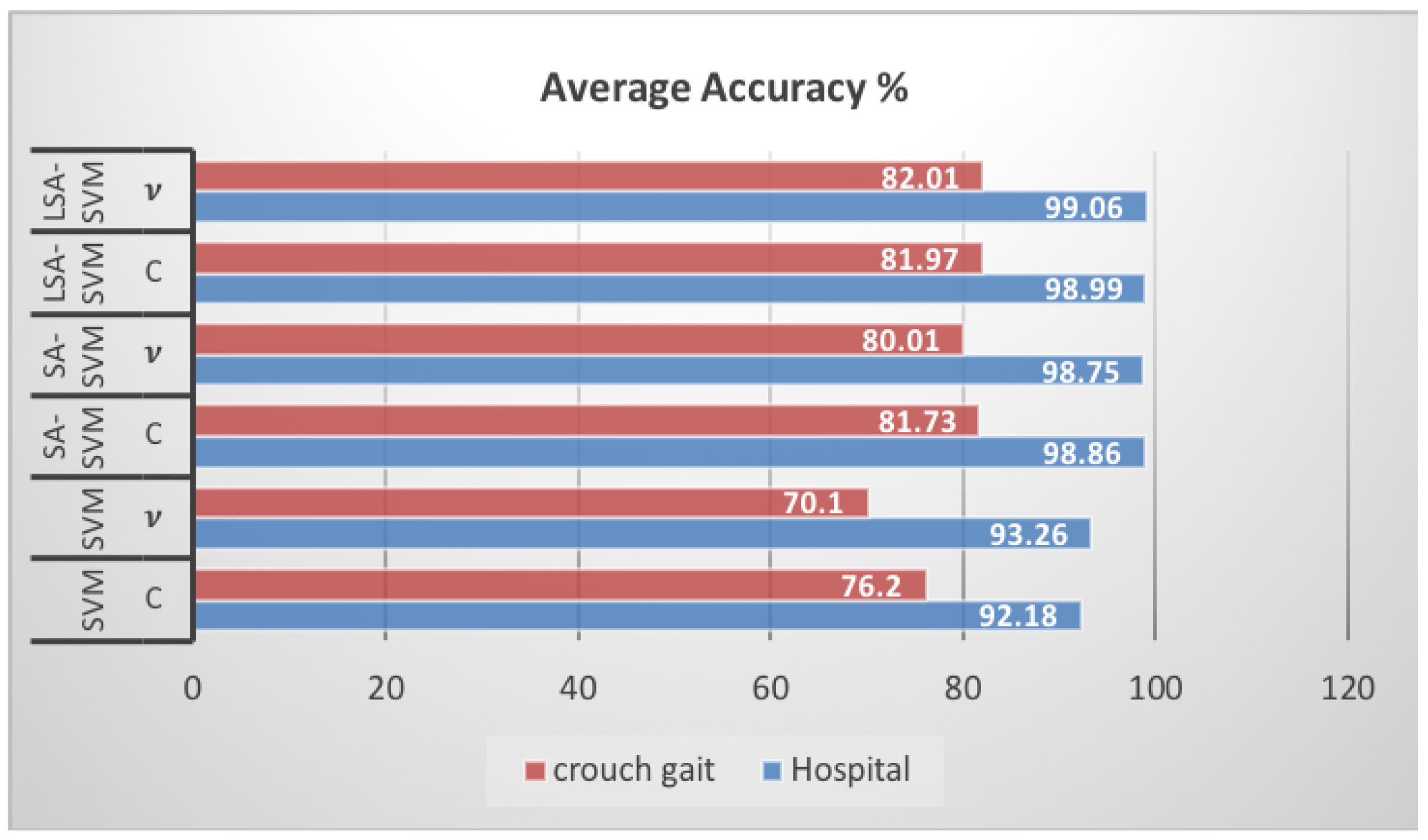
| SVM C | SVM v | SA-SVM C | SA-SVM v | LSA-SVM C | LSA-SVM v | |
| Hospital | 92.18 | 93.26 | 98.86 | 98.75 | 98.99 | 99.06 |
| crouch gait | 76.20 | 70.10 | 81.73 | 80.01 | 81.97 | 82.01 |
| Dataset | Training Time (ms) | |||||
|---|---|---|---|---|---|---|
| SVM C | SVM v | SA-SVM C | SA-SVM v | LSA-SVM C | LSA-SVM v | |
| Hospital | 55.3 | 54.3 | 107.9 | 46.3 | 70.7 | 69.4 |
| crouch gait | 48.5 | 55.1 | 36.3 | 38.0 | 48.9 | 48.4 |
| Dataset | Group | # Data | # Attributes |
|---|---|---|---|
| Iris | Small size | 100 | 4 |
| Parkinson | 195 | 22 | |
| Australian Credit Approval (Statlog) | Medium size | 689 | 4 |
| Breast Cancer | 699 | 9 | |
| Pima Indians diabetes | 768 | 8 | |
| Spambase | Large size | 4601 | 57 |
| Skin Segmentation | 245,057 | 3 |
| Dataset | C-SVM | v-SVM | Feat Type | Win. Size, Win. Inc. | ||
|---|---|---|---|---|---|---|
| C | C | |||||
| Iris | 1 | 1 | 1 | 0.25 | 11 | 20, 5 |
| Parkinson | 300 | 0.125 | 3000 | 0.003 | 14 | 50, 15 |
| Australian Credit Approval (Statlog) | 0.5 | 0.125 | 214 | 0.003 | 14 | 20, 5 |
| Breast Cancer | 8200 | 0.003 | 214 | 0.003 | 13 | 50, 7 |
| Spambase | 3000 | 0.003 | 2050 | 0.005 | 14 | 500, 120 |
| Pima Indians diabetes | 8200 | 0.0078 | 2050 | 0.002 | 14 | 50, 15 |
| Skin Segmentation | 100 | 0.003 | 1 | 2 | 14 | 500, 150 |
| Dataset | Accuracy (%) | |||||
|---|---|---|---|---|---|---|
| SVM C | SVM v | SA-SVM C | SA-SVM v | LSA-SVM C | LSA-SVM v | |
| Iris | 92.85 | 90.12 | 85.71 | 85.84 | 92.85 | 92.86 |
| Parkinson | 72.32 | 70.0 | 71.43 | 64.29 | 71.43 | 74.10 |
| Australian Credit (Statelog) | 81.6 | 80.8 | 88.07 | 88.53 | 91.28 | 96.42 |
| Breast Cancer | 89.88 | 88.76 | 90.96 | 90.33 | 92.09 | 91.01 |
| Pima Indians diabetes | 82.5 | 80 | 78.4 | 77.5 | 80.95 | 78.3 |
| Spambase | 61.17 | 62.52 | 61.18 | 62.53 | 62.19 | 61.26 |
| Skin Segmentation | 83.31 | 72.26 | 60.50 | 67.47 | 84.23 | 84.43 |
| Dataset | Training Time (ms) | |||
|---|---|---|---|---|
| SA-SVM C | SA-SVM v | LSA-SVM C | LSA-SVM v | |
| Iris | 0.837 | 0.701 | 3.6 | 4.1 |
| Australian Credit (Statelog) | 1.10 | 1.60 | 4.6 | 5.2 |
| Breast Cancer | 3.20 | 3.3 | 7.20 | 8.70 |
| Pima Indians diabetes | 0.901 | 0.836 | 5.0 | 4.7 |
| Spambase | 25.8 | 16.1 | 34.8 | 33.4 |
| Skin Segmentation | 121.4 | 86.3 | 267.2 | 133.1 |
© 2019 by the authors. Licensee MDPI, Basel, Switzerland. This article is an open access article distributed under the terms and conditions of the Creative Commons Attribution (CC BY) license (http://creativecommons.org/licenses/by/4.0/).
Share and Cite
Adil Abboud, S.; Al-Wais, S.; Abdullah, S.H.; Alnajjar, F.; Al-Jumaily, A. Label Self-Advised Support Vector Machine (LSA-SVM)—Automated Classification of Foot Drop Rehabilitation Case Study. Biosensors 2019, 9, 114. https://doi.org/10.3390/bios9040114
Adil Abboud S, Al-Wais S, Abdullah SH, Alnajjar F, Al-Jumaily A. Label Self-Advised Support Vector Machine (LSA-SVM)—Automated Classification of Foot Drop Rehabilitation Case Study. Biosensors. 2019; 9(4):114. https://doi.org/10.3390/bios9040114
Chicago/Turabian StyleAdil Abboud, Sahar, Saba Al-Wais, Salma Hameedi Abdullah, Fady Alnajjar, and Adel Al-Jumaily. 2019. "Label Self-Advised Support Vector Machine (LSA-SVM)—Automated Classification of Foot Drop Rehabilitation Case Study" Biosensors 9, no. 4: 114. https://doi.org/10.3390/bios9040114
APA StyleAdil Abboud, S., Al-Wais, S., Abdullah, S. H., Alnajjar, F., & Al-Jumaily, A. (2019). Label Self-Advised Support Vector Machine (LSA-SVM)—Automated Classification of Foot Drop Rehabilitation Case Study. Biosensors, 9(4), 114. https://doi.org/10.3390/bios9040114