1. Introduction
One of the most important needs in life is security, whether in normal day-to-day life or in the cloud world. The year 2017 witnessed a series of ransomware attacks (a simple form of malware that locks down computer files using strong encryption, and then hackers ask for money in exchange for release of the compromised files), targets including San Francisco’s light-rail network, Britain’s National Health Service, and even companies such as FedEx. One example is the WannaCry Ransomware Attack which compromised thousands of computers, and lately companies such as Amazon, Google, and IBM have started hiring the best minds in digital security so that their establishments across the world do not get easily compromised. Moreover, one can ask Amazon, Twitter, Netflix, and others about the Denial of Service attacks their servers faced back in 2016 [
1], in which the attackers flooded the system with useless packets, making the system unavailable. There were virtual machine escape attacks reported back in 2008 by Core Security Technologies, in which a vulnerability (CVE-20080923) was found in VMware’s (software developing firm named VMware Inc., Palo Alto, CA, USA) mechanism of shared folders, which made escape possible on VMWare’s Workstation 6.0.2 and 5.5.4 [
2]. The virtual-machine escape is a process of escaping the gravity of a virtual machine (isolated guest operating system) and then communicating with the host operating system. This can lead to a lot of security hazards. Attackers find new ways to exploit the network, and the security handlers need to be one step ahead by plugging all leakages beforehand. Many organizations are specially dedicated to come up with a security architecture that is robust enough to be employed in a clouding environment. Cato Networks (Israel), Cipher Cloud (San Jose, California), Cisco Security (San Jose, California), Dell Security (Texas) [
3], and Hytrust (California) are some of the organisations that are built with the sole purpose of making the cloud environment a safe place. Various researchers have put a lot of work into the field of cloud security and have proposed Intrusion Detection Systems (IDS) as a solid approach to tackle the issue of security. What an IDS does is that it captures and monitors the traffic and system logs across the network, and also scans the whole network to detect suspicious activities. Anywhere the IDS sees a vulnerability, it alerts the system or the cloud administrator about the possible attack. IDSs are placed at different locations in a network; if placed at the host, they are termed host-based IDSs (HIDS), while those placed at network points such as gateways and routers are referred to as Network based IDSs (NIDS). One employed at the Hyper-Visor (or VMM, Virtual Machine Monitor) is called the Hyper-Visor-based IDS (HVIDS). The HIDSs keep an eye on the VMs running and scan them for suspicious system files, system calls, unwanted configurations, and other irregular activities. The NIDS is basically employed to check for anomalies in the network traffic. The HVIDS is capable enough to filter out any threats looming over the VMs (Virtual Machines) that are running over the hypervisor. Some widespread techniques are Misuse detection techniques, in which already-known attack signatures and machine-learning algorithms are used to find out any mismatch with the captured data and any irregularities are reported. Similarly, in an anomaly detection, the system matches the behavioral pattern of data coming into the network with a desired behavioral pattern, and a decision is taken on letting the data flow further into the network or filtering it there and then. Thus, anomalies are detected. VMI is Virtual Machine Introspection in which programs running on VMs are scanned and dealt with. The VM introspection can be done in various ways such as kernel debugging, interrupt based, hyper-call authentication based, guest-OS hook based, and VM state access based. These all ways help to determine whether any suspicious programs are running at the low-level or high-level semantic end of the VM. There are many tools available such as Ether [
4] (a framework designed to do malware analysis, leveraging hardware virtualization extensions to remain hidden from malicious software), that help in performing this task from outside the VM. The traditional IDS techniques were vulnerable as they were basically employed from within the VM, but with VMI the chances of the VM being attacked are less as the introspection is being done from outside using VMM technology. The VMM software helps to create and run all VMs attached to it. It represents itself to attackers as being the targeted VM and prevents direct access to the physical hardware at the real VM. The VMI technique is employed at the VMM (privileged domain) that helps to keep an eye on other domains. The catch here is that the hypervisor or VMM itself may be attacked. For that scenario, HVI (Hyper-Visor Introspection) is developed; this depends mainly on hardware involvement to check the kernel states of the host and hypervisor operating system. Here, attacks such as rootkit, side-channel attacks, and hardware attacks can take place.
This paper will present a model through which various parameters related to the data are calculated, based on which an IDS could be developed to help secure the network.
Section 1 offers a brief introduction to the IDS and data integrity importance;
Section 2 discusses the motivation and reasons to pick up this subject as an area of research;
Section 3 covers a literature review related to the topic which will describe the various methods used to classify data;
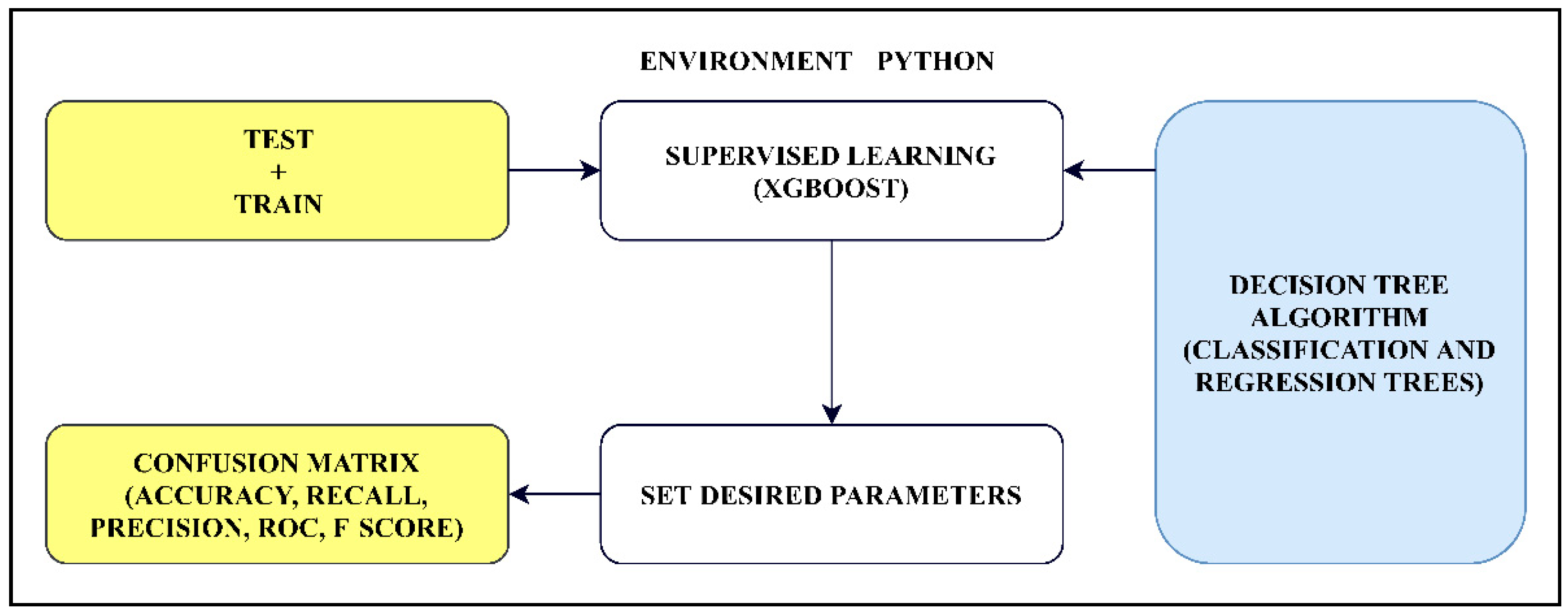
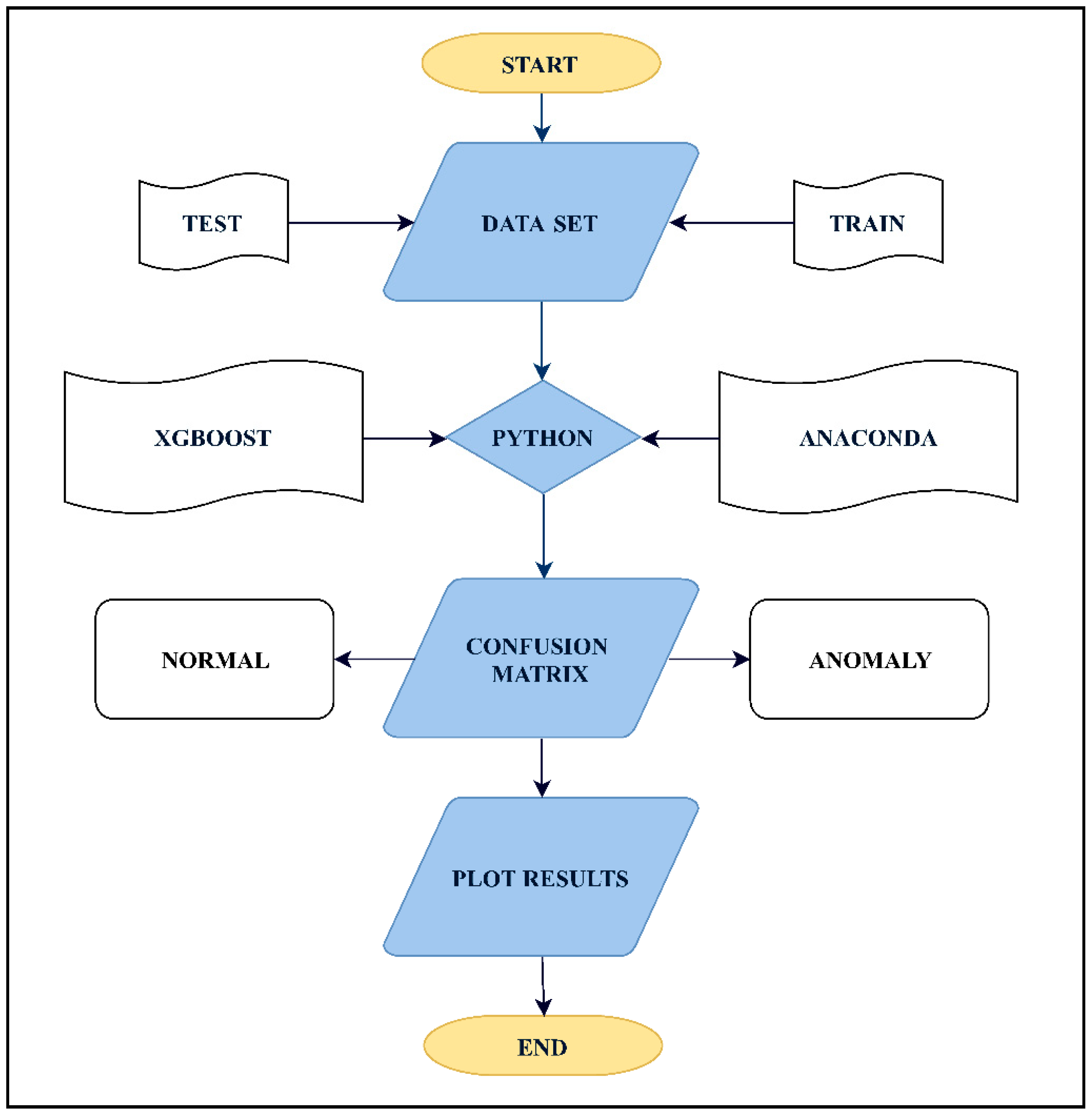
Section 4 represents the classification model used to carry out the results;
Section 5 offers more theory and background on the immediate techniques used in this paper, including decision trees, boosting, and XGBoost;
Section 6 explains the mathematical aspects of XGBoost and how the algorithm works in general;
Section 7 presents the main results achieved through the XGBoost algorithm on the NSL-KDD (network socket layer-knowledge discovery in databases) dataset; and finally
Section 8 concludes the paper.
3. Literature Review
Ektefa [
6] compared the C4.5 and SVM (Support Vector Machine) algorithms and, in the findings represented by him, C4.5 worked better for data classification. Most classifiers are based on the error rate, so they cannot be extended to multiclass complex real problems. Holden came up with a hybrid PSO (Particle Swarm Optimization) algorithm to deal with normal attribute values but it lacked many features [
7]. Ardjani used SVM and PSO together to optimize the performance of the SVM [
8]. As the data set used for an IDS is mostly multidimensional in nature, it is important to get rid of inconsistent and redundant features before extracting the features for classification of data. The selection of features through genetic algorithms gives a better result than when individually applied. Panda uses two major classification methods, namely, normal or attack [
9]. The combination of RBF (Gaussian Radial Basis Function) and the J48 algorithm (a type of greedy algorithm based on decision trees) has a higher RMSE (Root Mean Square Error) rate and is more prone to errors. Compared to this, Random Forest and Nested Dichotomies show a 99% detection rate and an error rate of a mere 0.06%.
Petrussenko Denis used LERAD (Learning Rules for Anomaly Detection) to detect attacks at the network level by using the network packets and TCP flow to learn about new attack patterns and the general trend of packet flow [
10]. He found that LERAD worked well using the DARPA (Defence Advanced Research Projects Agency) data set, giving a high detection rate. Mahoney used the various available anomaly methods like ALAD (Application Layer Anomaly Detector), PHAD (Packet Header Anomaly Detector), and LERAD (performed the best) to model the application, data-link, and other layers of the model [
11]. SNORT (developed by CISCO Systems), which is an open source IDS (used in collaboration with PHAD and NETAD) [
12], tested on the IDEVAL (Intrusion Detection Evaluation) data set detects up to 146 attacks out of a possible 201 attacks, when monitored for a week.
The Unsupervised method uses a huge volume of data and has less accuracy. To overcome this a semi-supervised algorithm is used [
13]. Fuzzy Connectedness-based Clustering is used using the properties of clusters such as Euclidean distance and statistics [
14]. This helps to detect known and unknown shapes. Ching Hao used unlabelled data in a co-training framework to better intrusion detection [
15]. Here a low error rate was achieved, which helped in setting up an active learning method to enhance the performance. The semi-supervised technique is used to filter false alarms and provides a high detection rate [
16].
To improve the accuracy, a Tri Training SVM algorithm is used [
17]. Adding further, Monowar H. Bhuyan used the tree-based algorithm to come up with clusters in the dataset without the use of labelled data [
18]. However, labelling can be done on the data set by using a cluster labelling technique which is based on the Tree CLUS (clusters) algorithm (works faster for numeric and other mixed datasets).
The Partially Observable Markov Decision Process was used to determine the cost function using both the anomaly and misuse-detection methods [
19]. The Semi-Supervised technique is then applied to a set of three different SVM classifiers and to the same PSVM (Principal SVM) classifiers.
DDoS, that is Distributed Denial of Service Attacks, are the most difficult to counter, as they are difficult to detect, but two ways are suggested to tackle them. The first way is to filter the traffic there and then by eliminating the mischievous traffic beforehand, and the second method is to gradually degrade the performance of the legitimate traffic. The major reason for the widespread DDoS attacks is the presence of Denial of Capability attacks. The Sink Tree model helps to eliminate these attacks [
20].
The DDoS attacks are not endemic to a network, but they harm the whole network. Zhang [
21] proposed a proactive algorithm to tackle this problem. Here, the network was divided into clusters, with packets needing permission to enter, exit, or pass through other clusters. The IP prefix-based method is used to control the high-speed traffic and detect the DDoS attacks, which come in a streaming fashion. There is some suggestion to use acknowledgment-based ways to supress intrusion. Here, the clock rates are synchronized with each other (client and server) and any lack or delay in the clock rates or acknowledgment loss allows the adversary to cause a direct attack on the client [
22].
Pre-processing the network data consumes time, but classification and labelling of data are the main challenges encountered in an IDS [
23]. Issues such as classification of data, high-level pre-processing, suppression, and mitigation of DDoS attacks, False Alarm Rates, and the Semi-Supervised Approach need to be dealt with to come up with a strong IDS model, and this paper is a step towards achieving it. Most of the classification methods discussed above had their own advantages and limitations, XGBoost was chosen because it helped in tackling majority of the flaws that emerged from the existing models. The reasons XGBoost is handpicked to be the preferred classification model when dealing with issues encountered in real word classification problems are the following:
XGBoost is approximately 10 times faster than existing methods on a single platform, therefore eliminating the issue of time consumption especially when pre-processing of the network data is done.
XGBoost has the advantage of parallel processing, that is uses all the cores of the machine it is running on. It is highly scalable, generates billions of examples using distributed or parallel computation and algorithmic optimization operations, all using minimal resources. Therefore, it is highly effective in dealing with issues such as classification of data and high-level pre-processing of data.
The portability of XGBoost makes it available and easier to blend on many platforms. Recently, the distributed versions are being integrated to cloud platforms such as Tianchi of Alibaba, AWS, GCE, Azure, and others. Therefore, flexibility offered by XGBoost is immense and is not tied to a specific platform, hence the IDS using XGBoost can be platform-independent, which is a major advantage. XGBoost is also interfaced with cloud data flow systems such as Spark and Flink.
XGBoost can be handled by multiple programming languages such as Java, Python, R, C++.
XGBoost allows the use of wide variety of computing environments such as parallelization (tree construction across multiple CPU Cores), Out of core computing, distributed computing for handling large models, and Cache Optimization for the efficient use of hardware.
The ability of XGBoost to make a weak learner into a strong learner (boosting) through its optimization step for every new tree that attaches, allow the classification model to generate less False Alarms, easy labelling of data, and accurate classification of data.
Regularization is an important aspect of XGBoost algorithm, as it helps in avoiding data overfitting problems whether it be tree based or linear models. XGBoost deals effectively with data-overfitting problems, which can help to deal when a system is under DDoS attack, that is flooding of data entries, so the classifier is needed to be fast (which XGBoost is) and the classifier should be able to accommodate data entries.
There is enabled cross-validation as an internal function. Therefore, there is no need of external packages to get cross validation results.
XGBoost is well equipped to detect and deal with missing values.
XGBoost is a flexible classifier as it gives the user the option to set the objective function as desired by setting the parameters of the model. It also supports user defined evaluation metrics in addition to dealing with regression, classification, and ranking problems.
Availability of XGBoost at different platforms makes it easy to access and use.
Save and Reload functions are available, as XGBoost gives the option of saving the data matrix and relaunching it when required. This eliminates the need of extra memory space.
Extended Tree Pruning, that is, in normal models the tree pruning stops as soon as a negative loss is encountered, but in XGBoost the Tree Pruning is done up to a maximum depth of tree as defined by the user and then backward pruning is performed on the same tree until the improvement in the loss function is below a set threshold value.
All these important functionalities add up and enable the XGBoost to outperform many existing models. Moreover, XGBoost has been used in many winning solutions in machine learning competitions such as Kaggle (17 out of 29 winning solutions in 2015) and KDDCup (top 10 winning solutions all used XGBoost in 2015) [
24]. Therefore, it can be said that XGBoost is very well equipped to deal with majority of the problems that face a real-world network.
6. Mathematical Explanation
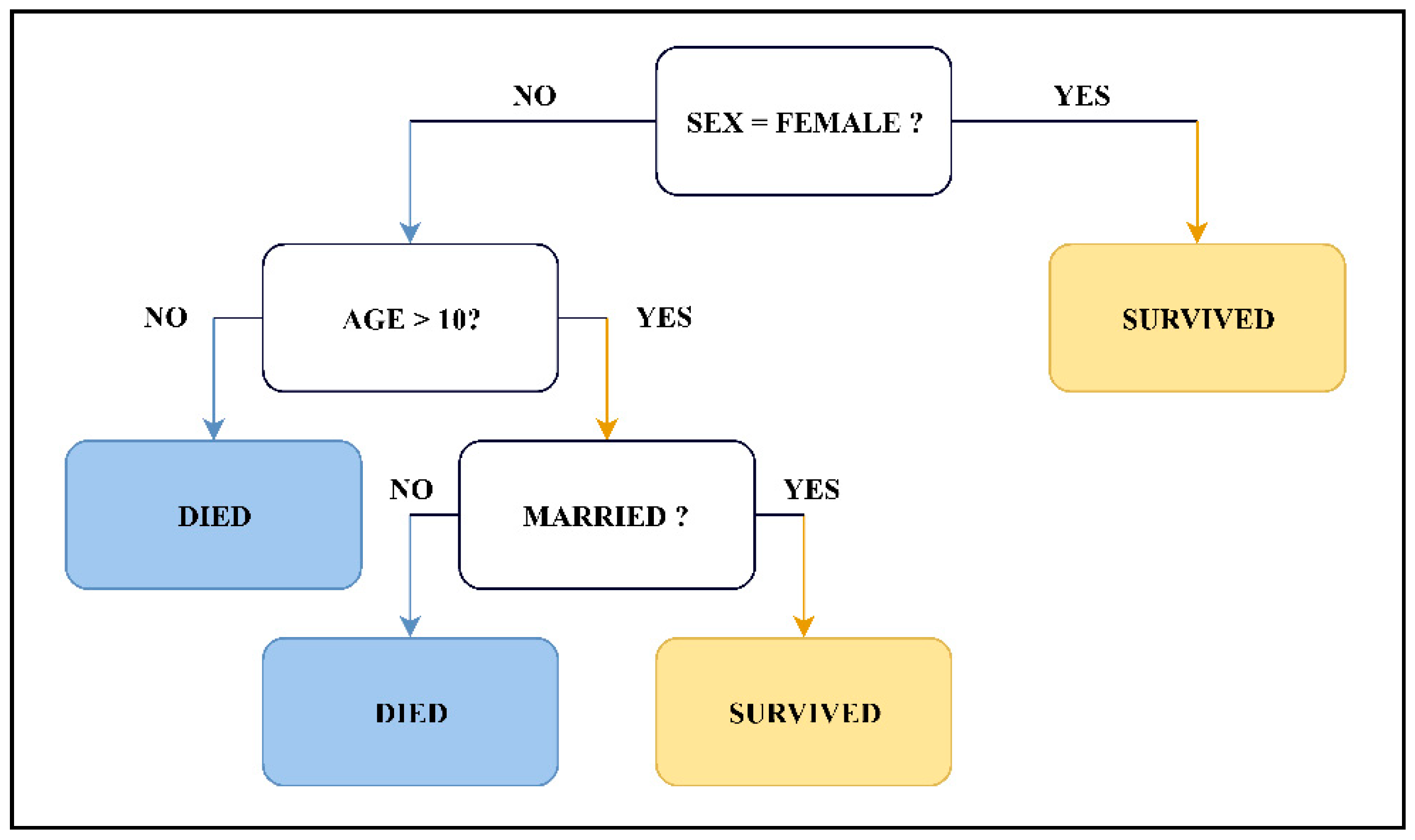
XGBoost functions around tree algorithms. The tree algorithms take into account the attributes of the dataset; they can be called features or columns and then these very features act as the conditional node or the internal node. Now, corresponding to the condition at the root node, the tree splits up into branches or edges. The end of the branch that does not produce any further edges is referred to as the leaf node, and generally splitting is done to reach a decision. The diagram in
Figure 4 is a representation of how a decision tree or classification tree works, based on an example dataset, predicting whether a passenger survives or not.
XGBoost also applies decision-tree algorithms to a known dataset and then classifies the data accordingly. The concept of XGBoost revolves around gradient-boosted trees using supervised learning as the principal technique. Supervised learning basically refers to a technique in which the input data, generally the training data having multiple features (as in this case), is used to predict target values
The mathematical algorithm (referred to as the model) makes predictions
based on trained data
. For example, in a linear model, the prediction is based on a combination of weighted input features such as
=
[
29]. The parameters need to be learnt from the data. Usually,
is used to represent the parameters and, depending on the dataset, there can be numerous parameters. The predict value
helps to classify the problem at hand, whether it be regression, classification, ranking, or others. The main motive is to find the appropriate parameters from the dataset used for training purposes. An objective function is set up initially which describes the model performance. It must be mentioned that each model can differ depending on which parameter is used. Suppose that there is a dataset in which “length” and “height” are features of the dataset. Therefore, on the same dataset numerous models can be set up, depending on which parameters are used.
The objective function [
29] comprises two parts: the first part is termed a training loss and the second part is termed a regularization.
The regularization term is represented by R and TL is for Training Loss. The TL is just a measure of how predictive the model is. Regularization helps to keep the model’s complexity within desired limits, eliminating problems such as over-stacking or overfitting of data which can lead to a less accurate model. XGBoost simply adds the prediction of all trees formed from the dataset and then optimizes the result.
Random Forest also follow the model of tree ensembles. Therefore, it can be said that the boosted trees, in comparison to random forest, are not too much different in terms of their algorithmic make-up, but they differ in the way we train them. A predictive service of tree ensembles should work both for random and boosted trees. This is a major advantage of supervised learning. The main motive is to learn about the trees, and the simple way to do it is to optimize the objective function [
29].
The question that arises here is how the trees are set up in terms of the parameters used. To determine these parameters the structure of the trees and their respective leaf scores are to be calculated (generally represented by a function
). It is not a straightforward task to train all the trees in parallel. XGBoost tries to optimize the learned tree (training) and adds a tree at every step. One question that arises is which tree to add at each step, the answer being to add the tree that fulfills the objective of optimizing our objective function [
29].
The new objective function (say at step
t) takes the form of an expansion represented by Taylor’s theorem, generally including up to the second order.
where
and
are taken as inputs.
The result reflects the desired optimization for the new tree that wants to add itself to the model. This is the way that XGBoost deals with loss functions such as logistic regression.
Moving further, regularization plays an important part in defining the complexity of the tree
R(f). The definition of tree
f(p) can be refined as [
29]
In the above equation,
represents a vector for leaf scores (same score for data points using the same leaf) and function
q assigns leaves to the corresponding data points.
L is the number of leaves. In XGBoost, the complexity is [
29]
Therefore, the equation of regularization can be put in Theorem (1), to get the new optimized objective function at step t, or the tth tree. The resultant model represents the new reformed tree model and is a measure of how good the tree structure q(p) is.
The tree structure is established by calculating the regularization, leaf scores, and objective function at each level, as it is not possible to simultaneously calculate all combinations of trees. The gain is calculated at each level as a leaf is split into a left leaf and a right leaf, and the gain is calculated at the current leaf with the regularization achieved at the possible additional leaves. If the gain falls short of the additional regularization value, then that branch is abandoned (concept also called pruning). This is how XGBoost runs deep into trees and classifies data, and hence accuracy and other parameters are calculated.
7. Results and Discussion
7.2. Confusion Matrix
XGBoost has many parameters, and one can use these parameters to perform specific tasks. The following are some of the parameters that were used to get the results (the purpose of the parameters is also explained briefly) [
31]:
The “learning_rate” (also referred to as “eta”) parameter is basically set to get rid of overfitting problems. It performs the step size shrinkage, and weights relating to the new features can be easily extracted (was set as 0.1).
The “max_depth” parameter is used to define how deep a tree runs: the bigger the value, the more complex the model becomes (was set as 3).
The “n_estimators” parameter refers to the number of rounds or trees used in the model (was set as 100).
The “random_state” parameter is also a learning parameter. It is also sometimes referred to as “seed” (was set as 7).
The “n_splits” parameter is used to split up the dataset into k parts (was set as 10).
The above-mentioned parameters are tree booster parameters and based on the above the following results were calculated. There are many parameters that can be set up, but this mainly depends on the user and the model. If parameters are not set, XGBoost picks up the default values, though one can define the parameters as per the desired model.
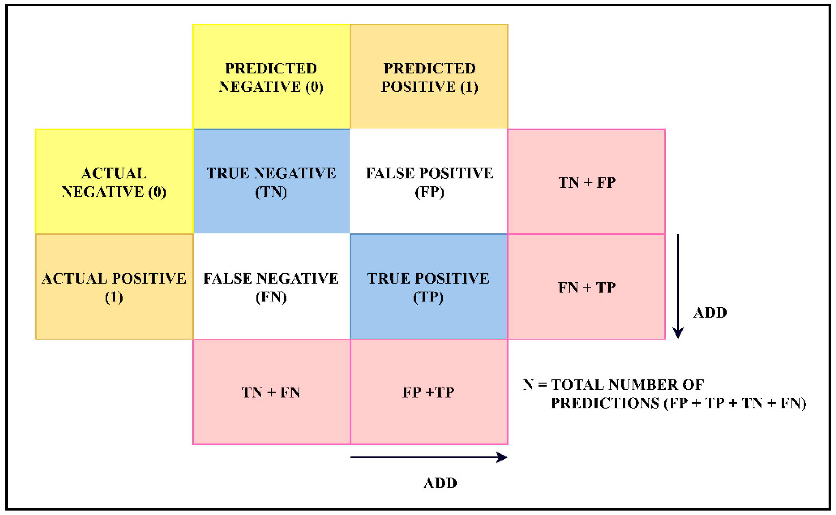
The matrix in
Figure 5 represents what a confusion matrix is made up of.
The quantities defined in
Figure 5 will be used to calculate all the results achieved. There are four main values, which are calculated by running the confusion matrix. These values are further used to calculate the accuracy, precision, recall, F1 score, and ROC curve, and finally plot the confusion matrix itself.
To elaborate, there are four main values: True Negative (TN) (negative in our dataset was the target name “anomaly” labelled as 0), True Positive (positive in our dataset was the target name “normal” labelled as 1), False Negative, and False Positive.
True Positive is a value assigned to an entry of the dataset when a known positive value is predicted as positive, in other words if the color is red, and is predicted as red. True Negative is when a known negative value is predicted as negative, that is the color is not red and is predicted as being not red. On the other side, there are False Negative and False Positive. False Positive is when a known positive value is predicted as negative, that is a known red color is predicted as not being red. False Negative is the other way around, a known negative value is predicted as positive, that is the red color is predicted when the known color was not red.
The Confusion Matrix represents the quality of the output of a classifier on any dataset. The diagonal elements (blue box in
Figure 5 and
Figure 6) represent correct or true labels, whereas the off-diagonal (white box in
Figure 5 and
Figure 6) elements represent the elements misclassified by the classification model. Therefore, the higher the values of the diagonal elements of the confusion matrix, the better and more accurate the classification model becomes.
Figure 6 represents the confusion matrix in normalized form, that is in numbers between 0 and 1. It provides better and easier understanding of the data.
The different parameters of the Confusion Matrix represent the results giving TP, TN, FP, and FN. Using these, the specificity and sensitivity of the dataset can be calculated, which is just a measure of how good the classification model is. The following were the results from the confusion matrix:
TP = 99.11% (0.991123108469).
FP = 1.75% (0.0174775758085).
FN = 0.89% (0.00887689153061).
TN = 98.25% (0.982522424192).
FP and FN should be as low as possible, whereas TP and TN should be as high as possible. The model is a good classification model as there is a high fraction of correct predictions as compared to the misclassifications. Moreover, the sensitivity and specificity can be calculated.
Sensitivity = TP/(FN + TP) (also called TPR)
= 99.11%.
Specificity = TN/(TN + FP)
= 98.25%
Therefore, FPR can be calculated:
FPR = (1 − specificity)
= (1 − 0.9825)
= 0.0175
As a cross-check, looking at
Figure 5,
TN + FN + FP + TP = N is the total number of predictions. If we apply this formula, taking values from
Figure 6, then the result comes out to be
N = (
TN + FN + FP + TP) = (70,214 + 684 + 1249 + 76,370), the representation of values in non-normalized form = 148,517, that is the total number of entries (rows) in the combined dataset. Therefore, the result obtained from the Confusion Matrix validates the dataset entries.
The confusion matrix is the heartbeat of the classification model. Looking at the results above, the classification model achieves very good results, but more parameters can be set up and the best possible accuracy should be aimed at. The higher the values of TN and TP and the lower the values of FN and FP, the stronger the model emerges. It must be mentioned here that this classification model can form an integral part of an IDS in helping it to classify data as anomaly or normal. The confusion matrix can be a source of data from which optimization of the model can be initiated. By setting up more-specific parameters, accuracy, precision, recall, and other results can be optimized to achieve perfect results.
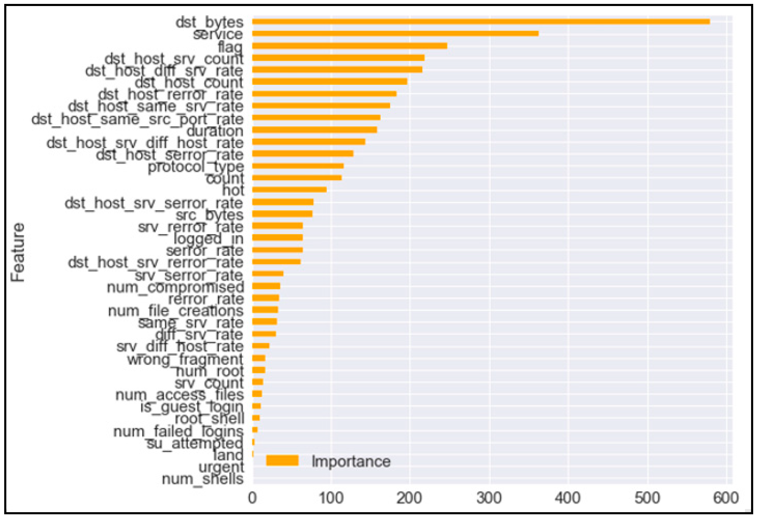
7.5. Feature Score (F-Score)
Moving further, using an in-built function, the feature importance was also plotted.
Figure 9 represents the result achieved.
Table 3 represents the meaning of the features used in the dataset [
35].
Figure 9 showed that the feature representing “dst_bytes” was the most important attribute as it had the highest F-score, and on the other hand, “num_shells” was the least important attribute as it had the lowest F-score. It must be noted that the F-score was calculated by setting up a model having parameters defined as:
“learning_rate”—0.1, “max_depth”—5, “sub-sample”—0.9, “colsample_bytree”—0.8, “min_child_weight”—1, “seed”—0, and “objective”: “binary: logistic” (Why are these specific values chosen? Look at
Table 4 and
Table 5).
The following are some of the additional parameters used and their meaning:
The “min_child_weight” parameter defines the required sum of instance weight in a child. If the sum of instance weights in a leaf node falls short of this parameter, further steps are abandoned.
The “subsample” parameter allows XGBoost to run on a limited set of data and prevents overfitting.
The “colsample_bytree” parameter corresponds to the ratio of columns in the subsample when building trees.
The “objective”: “binary: logistic” parameter is a learning parameter and is used to specify the task undertaken: in this case uses logistic regression for binary classification.
It must be mentioned that various combinations of parameters having different values were run, and every time the attribute importance did not change for the most important attribute, as “dst_bytes” received the highest F-score each time the parameter values were changed. However, the least important end changed with a change in parameter values. So, it can be said that the parameters did have a direct effect on the F-scores of the attributes, as any change in parameters reflected a change in the F-score of the attributes in the NSL-KDD dataset. We set up the model parameters as above, as running the code with these values had given the best results in terms of mean and standard deviation. This will be elaborated further.
The following were some of the F-scores using the above-mentioned parameters:
“dst_bytes”—this attribute of the dataset accounted for the highest F-score of about 579.
“num_shells” and “urgent”—this attribute of the combined test and train dataset accounted for the least F-score of 1.
Further, more features were extracted out of the dataset importing GridSearchCV from the sklearn package. This functionality of sklearn enabled us to evaluate the grid score, which showed the mean and the corresponding standard deviation of the dataset using parameters such as “subsample”, “min_child_weight”, “learning_rate”, “max_depth”, and others. The following were some of the results:
Two models were run. In the first model, the following were fixed parameters: “objective”: “binary: logistic”, “colsample_bytree”—0.8, “subsample”—0.8, “n_estimators”—1000, “seed”—0, “learning_rate”—0.1. The model was run to calculate the best values of the mean and the corresponding standard deviation for different combinations of the parameters “min_child_weight” and “max_depth”.
Table 4 represents the result achieved.
From the above, it can be seen that the highest mean was 0.99921 achieved when the “min_child_weight” and “max_depth” parameters were set as 1 and 5, respectively; therefore, these parameter values were used while plotting the feature score (
Figure 9).
In the second model, the following parameters were fixed: “min_child_weight”—1, “seed”—0, “max_depth”—3, “n_estimators”—1000, “objective”: “binary: logistic”, “colsample_bytree”—0.8. The model was run to calculate the best values of mean and standard deviation for different combinations of the parameters of “learning_rate” and “subsample”.
Table 5 represents the result achieved.
From the above, it can be seen that the highest mean was 0.99917, achieved when the “learning_rate” and “subsample” parameters were set as 0.1 and 0.9, respectively.
The higher the value of the mean the better the accuracy of the model is, and hence the better the readings will be reflected at the confusion matrix, ROC, precision, and recall results. Looking at models 1 and 2, the parameters were set up and the F-score was calculated as seen in
Figure 9. Therefore, now it can be understood why the parameters as discussed in the feature score (
Figure 9) were set up, as they accounted for higher mean values as seen in models 1 and 2, though one can choose a new model by assigning parameter values as desired and based on those very values the F-score can be calculated.
There can be many combinations to find the best parameter values used to set up a final model. The whole motive is to find a model which gives the best results. The higher the mean values, the better the model is to predict accuracy and other targets. The above two models were run to just know the effect of parameters on a model. The best-fit values can be extracted and used in future models so that accuracy reaches close to 100%. Every model has a different feature score; all it depends on is the value of parameters set. Models 1 and 2 were run and, extracting from these two models the best-fit parameters, a final model was set up. The feature score was plotted in relation to the final model as seen in
Figure 9.
8. Conclusions
The prediction of data is excellent in this classification model (Accuracy = 98.70%) and based on this, future research could be set up which can help in initiating models designed to detect intrusions. This research can help to design an IDS of the future, especially when security remains such an issue. The findings are a reflection as to how effective and accurate XGBoost is when it comes to predicting a dataset. The findings are very accurate, and the error rate is very low. These findings can be further elaborated to design Intrusion Detection Systems which are robust and can be employed in architectures of the future such as IoT, 5G, and others.
A lot of work has been done in the field of classification models and their importance when it comes to the classification of data. As discussed earlier, classification methods such as SVMs, RBF, Neural Networks, Decision Trees, and others have been tested to classify data. Even the hybrid models have come up which employ more than one methods. Many researches have been carried out and as compared to most of the classification methods XGBoost gives relatively higher results. XGBoost is a relatively new concept as compared to others and its results are making it a model to investigate. Random Forests and hybrid models do come close to the accuracy achieved by XGBoost classification method when employed on NSL-KDD dataset, but in a real environment the type of data in a network will be different and that brings to the main question as to which classification method to adopt. Countering this question many investigators have majorly tried to compare the RF techniques and the XGBoost technique on various datasets, and the results give XGBoost an edge over the RF counterpart. The other important thing is that the RF are very prone to overfitting, and to achieve a higher accuracy, RF needs to create high number of decision trees, and moreover the data needs to be resampled again and again, with each sample requiring to train the new classifier. The different classifiers generated try to overfit the data in a different way, and voting is needed to average out those differences. The re-training aspect of RF is eliminated in XGBoost techniques, which basically add a new classifier to the already trained ensemble. This may seem a small difference between the two techniques but when they will be applied to an IDS, then they can affect the performance and complexity of the IDS in a big way. The only difference is that the XGBoost requires more care in setting up.
Moving further, there are a few more things that add weight to XGBoost as being a perfect classification method as this algorithm provides accuracy, feasibility, and efficiency. It automatically can operate in parallel on Windows and Linux (has both linear model solver as well as tree learning algorithms) and is up to 10 times faster than the traditional GBM (Generalized Boosted Models). Xgboost offers flexibility as to what type of input it can take, also accepts sparse input for both tree and linear booster. XGBoost also supports customized objective and evaluation functions. As a real-life application example, XGBoost has been widely adopted in industries such as Google, Tencent, Alibaba, and more, solving machine learning problems involving Terabytes of real life data.
The success and impact of the XGBoost algorithm is very well documented in numerous machine learning and data mining competitions. As an example, the records from machine learning competition site “Kaggle”, show that majority of winning solutions use XGBoost (17 winning solutions out of 29 used XGBoost in 2015). In the KDDCup competition in 2015, XGBoost was used by every winning team in the top 10. The winning solutions were solutions to problems such as malware classification; store sales prediction; motion detection; web text classification; customer behaviour prediction; high energy physics event classification; product categorization; ad click through rate prediction; hazard risk prediction, and many others. So, it can be well established that the datasets used in these solutions differed and many problems such as False Alarms, classification of data, and high-level pre-processing were dealt with, but the only thing that remained constant was the use of “XGBoost” as the preferred classification technique (especially when it came to the choice of learner).
Many E-Commerce companies have also adopted XGBoost as the classification method for various purposes, as seen by a leading German fashion firm (ABOUT YOU) employing XGBoost to do return prediction in a faster and robust way. The company was able to process up to 12 million rows in a matter of minutes achieving a high accuracy in predicting whether a product will be returned or not.
These are a few examples and XGBoost’s capability to use cloud as a platform makes it a hit in emerging markets. The new technologies are all based around the concept of cloudification and virtualization, and this is where XGBoost has an advantage. As its flexibility, no specific platform need, multiple accessible languages, availability, high quality results in less time, handling of sparse entries, out of core capability and distributed structure make it a well-suited classification method (consumes less resources on top of that).
The most important factor that emerges in classification problems is the scalability and this is where XGBoost is best at. It is highly scalable algorithm. It runs approximately ten times faster than existing methods on a single platform, and scales to millions and billions of examples as per the memory settings. The scalability is achieved through the algorithmic optimizations and smart innovations such as: a unique tree learning algorithm for handling sparse data; a weighted quantile procedure to handle the instance weights in approximate tree learning; the use of parallel and distributed computation leading to quick learning which makes the model exploration faster; and one of the most important strengths of XGBoost is the ability to provide out of core computation which allows the data scientists to process data including billions of examples on a cheap platform such as desktop.
These advantages have made XGBoost a go-to algorithm for Data Scientists, as it has already shown tremendous results in tackling large scale problems. Its properties such as user-defined objective function make it highly flexible and versatile tool that can easily solve problems related to classification, regression, and ranking. Moreover, as an open source software, it is easily available and accessible from different platforms and interfaces. This amazing portability of XGBoost allows compatibility with major Operating Systems therefore breaking static properties of previously known classification models. The new functionality that XGBoost offers is that it supports training on distributed cloud platforms, such as AWS, GCE, Azure, and others. This is a major advantage as the new technologies related to IoT and 5G is all built around cloud, and XGBoost is also easily interfaced with cloud dataflow systems such as Spark and Flink. XGBoost can be used through multiple programming languages such as Python, R, C++, Julia, Java, and Scala. XGBoost has already proven to push the boundaries of computing power for boosted tree algorithm as it lays special attention to model performance and computational speed. On a financial front, XGBoost systems consume less resources as compared to other classification models, they also help in saving and reloading of data whenever required. The implementation of XGBoost offers advanced features for algorithm enhancement, model tuning, and computing environments. The assessment of all classification methods leads to the choice of XGBoost being used as the classification method as it can solve real world scale problems using less resources. The impact of XGBoost cannot be neglected and it can be said that XGBoost employed as an integral part of IDS performing functions as described above can emerge as a stronger classification model than many others.
The focus is to build a strong classification model for use in IDS. A strong classification model means one which can give near-perfect results. This will lead to a stronger IDS, which, when deployed in a certain network, will make it more secure and there will be much fewer chances of intrusion as the classification model running is of very high standard. The next bit is using the IDS as a sensor to alert the administrator about any irregularities. The IDS can be used as a one- stop device to extract information about the network. So, IDS can also act as a data source and its machine learning capabilities make it a flexible technology, avoiding regular updating. The IDS in future can also be made interactive with IoT devices. It can also form an integral part of Artificial Intelligence, as security is also a problem in the robotic world (even robots can be hacked). Airplanes, cars, mobile networks, the world of IoT, Artificial Intelligence, and smart devices all need IDS sensors employed in their architecture. Basically, anything that has internet and machines involved can use IDS as a security feature.
The future world needs its privacy intact, so the developing robotic technology that will do a lot of work in future needs IDS. There is nothing perfectly safe in a network and there must be an IDS in a network to monitor everything, as people travelling in planes, cars, etc. should be able to trust the machines that are responsible for dropping them home. For example, any hacking resulting in a plane getting hijacked due to intrusions in the network can lead to devastating results.
To summarize, XGBoost needs to be a go-to classification method because it offers flexibility and can simultaneously work on different operating systems, gives a higher accuracy, can accept diverse data as inputs, offers both linear model solver and tree algorithms, and finally has been deployed in industries to tackle Terabytes of data. Therefore, it is already accepted in society and is giving tremendous results.


