Article

Vector Spatial Big Data Storage and Optimized Query Based on the Multi-Level Hilbert Grid Index in HBase

1
School of Earth Sciences, Zhejiang University, 38 Zheda Road, Hangzhou 310027, China
2
School of Architectural and Surveying & Mapping Engineering, JiangXi University of Science and Technology, 86 Hongqi Avenue, Ganzhou 341000, China
3
Zhejiang Provincial Key Laboratory of Geographic Information Science, 148 Tianmushan Road, Hangzhou 310028, China
4
Institute of Remote Sensing and Digital Earth, Chinese Academy of Science, Beijing 100101, China
*
Author to whom correspondence should be addressed.
Information 2018, 9(5), 116; https://doi.org/10.3390/info9050116
Submission received: 16 March 2018 / Revised: 28 April 2018 / Accepted: 4 May 2018 / Published: 9 May 2018

Abstract

:
Faced with the rapid growth of vector data and the urgent requirement of low-latency query, it has become an important and timely challenge to effectively achieve the scalable storage and efficient access of vector big data. However, a systematic method is rarely seen for vector polygon data storage and query taking spatial locality into account in the storage schema, index construction and query optimization. In the paper, we focus on the storage and topological query of vector polygon geometry data in HBase, and the rowkey in the HBase table is the concatenation of the Hilbert value of the grid cell to which the center of the object entity’s MBR belongs, the layer identifier and the order code. Then, a new multi-level grid index structure, termed Q-HBML, that incorporates the grid-object spatial relationship and a new Hilbert hierarchical code into the multi-level grid, is proposed for improving the spatial query efficiency. Finally, based on the Q-HBML index, two query optimization strategies and an optimized topological query algorithm, ML-OTQ, are presented to optimize the topological query process and enhance the topological query efficiency. Through four groups of comparative experiments, it has been proven that our approach supports better performance.

1. Introduction

The advancement of spatial information acquisition technologies and the proliferation of geographical information applications result in an explosive growth of spatial vector data. The traditional centralized data management technologies are facing the problems of high-concurrent read-write and the scalability problem while dealing with massive and complex spatial vector data. How to achieve scalable storage and fast query at low costs is an urgent and challenging issue. Cloud computing is a new distributed computing and storage architecture that supports a massive horizontal extension on low-cost computers, which provides infinite and scalable storage and computing power. Applying cloud computing to the geographic information system (GIS) is an effective way to solve massive spatial vector data issues [1,2,3,4].
HBase [5] is a highly scalable, high-concurrency, high-reliability and fault-tolerant distributed column-oriented NoSQL database, built on top of the Hadoop Distributed File System (HDFS) [6], providing powerful storage capacity and offering low-latency query service. In vector data management, operations are processed frequently and require low latency, especially for query operations; whereas, HDFS is mainly suitable for big block data storage, low-frequency update and allowing response latency. Therefore, HDFS alone has difficulty solving the massive spatial vector data storage issue. In contrast, HBase is suitable for massive vector data storage and retrieval scenarios and also can be extended with third-party SQL components to support standard SQL operations. Specifically, first, HBase is designed to achieve unstructured and semi-structured big data storage, support fast query and frequent update and allow single or batch delete and insertion anywhere. In addition, it also supports MapReduce for distributed computing. Thirdly, HBase is a column-based sparse row/column matrix that does not store elements with empty column values, saving significant storage space. Fourthly, the rowkey of HBase can be designed flexibly according to different applications. Finally, based on the SQL query component such as Apache Phoenix [6], the HBase database can be operated via standard SQL statements and integrated seamlessly with application systems based on traditional relational databases.
In the field of vector spatial data storage and fast query, a systematic method for HBase storage-schema design and index construction, especially for the design of rowkeys, has become an urgent and significant problem. Most of the previous works focused on the point data model [2,4,7], and works on the polygon data model are rarely seen. In addition, for the spatial index, more representative methods include R-tree [8,9], grid [10,11], quadtree [12], and so on, but the query, delete and insert operations in R-tree are more complex. The grid index maintains data locality and is more suitable for point data storage, but it easily increases redundancy for line and polygon data and cannot solve the multi-scale issue. As the quadtree index becomes deeper and does not maintain data locality, the data that are accessed are more unrelated to the query, reducing performance. Finally, few approaches are proposed to optimize query processing.
To address the above issues, a new approach for vector polygon big data storage and fast query based on HBase is proposed. Not only are we concerned about the design of the rowkey, but we propose a new index structure and query optimization strategies to improve query efficiency. Firstly, in the vector data storage model, the rowkey in the HBase table is the concatenation of the Hilbert value of the grid cell in which the object entity belongs, the layer identifier and the order code. Such a rowkey design shows the advantages of keeping spatial data proximity storage on disks and flexibly supporting the fast query based on layers. Secondly, a new multi-level grid index structure termed quadtree-Hilbert-based multi-level index (Q-HBML) that incorporates the grid-object spatial relationship (partial coverage and coverage) and a new Hilbert hierarchical code into a multi-level grid is proposed for indexing the information of multi-scale vector data and improving the efficiency of spatial query, and a new generation algorithm for the Hilbert code is put forward to encode hierarchical Q-HBML grid cells. Such an index design avoids the drawbacks of a latitude-longitude grid by dividing a large geographic space into levels in the quadtree structure and takes advantage of the localization and hierarchical feature of the Hilbert curve to directly encode grid cells without using a two-level index structure. Finally, based on the grid-object spatial relationship in the Q-HBML index, two query optimization strategies and a multi-level index based optimized topological query algorithm (ML-OTQ), are presented to optimize the spatial topological query processing and enhance the spatial query efficiency.
The rest of this paper is organized as follows. Section 2 introduces the related works. Section 3 presents the data storage schema for vector spatial data. Section 4 proposes a new multi-level grid spatial index and the optimized query strategies. Section 5 experimentally illustrates their efficiency. Section 6 concludes the paper.

2. Related Works

Recently, there have been some studies on vector big data storage and query based on HBase, primarily including three aspects: the storage model, spatial index and query process. The design of the storage model and spatial index plays a vital role in an efficient query. On the one hand, most previous researchers focused on the design of the point data storage model [2,4,7]. Zhang et al. [2] designed the vector distributed storage and index model for point data in HBase. It used the vector data record ID as the HBase rowkey and adopted the grid spatial index to construct the spatial index. Experiments showed that their method performed better compared with MongoDB and MySQL. Nishimura et al. [4] designed a multi-dimensional index based on K-d tree and quadtree for location services. In the above studies, the grid index is simple and more suitable for point data storage, but it easily increases the redundancy for line and polygon data. On the other hand, a few researchers started to design a polygon storage model, which is more complex. Wang et al. [1] proposed two HBase storage schemas for polygon data. The first was the storage schema with rowkeys based on the Z-curve, and the second was the storage scheme with rowkeys based on geometry object identifiers. Experiments demonstrated that building a spatial index in rowkeys was a better choice than building it in columns to improve the efficiency of region query. However, this work increases the storage space owing to the storing of an object more than once and ignores the cases in which a grid cell may belong to many vector objects, resulting in the non-uniqueness of rowkeys in the first storage schema. The Hilbert curve is proven to perform better data locality mapping than the Z-curve and improves the spatial retrieval efficiency, which has been applied in the fields of spatial data partition [13,14] and the vector storage schema [3]. Wang and Hong et al. [14] proposed a new algorithm for the generation of Hilbert code by studying the Hilbert curve, and the Hilbert code was applied to the spatial partition for massive spatial data. Faloutsos et al. [15] proposed the use of the Hilbert code, presenting that the good distance-preserving mappings can improve the performance of a spatial index and a spatial query and demonstrated that the Hilbert code achieved better clustering than Z-ordering (actually, the Peano curve) and bit-shuffling. Wang et al. [3] designed a vector spatial data model based on HBase. The Hilbert value and entity ID were denoted as the rowkey in the HBase table, and they proposed a parallel method of building the Hilbert R-tree index using MapReduce. However, the Hilbert curve is rarely used in the field of the spatial index.
For the spatial index, Shaffer et al. [16] designed a prototype geographic information system that used the quadtree to represent point, line and polygon data. Li et al. [17] presented a hybrid structure of the spatial index based on the multi-grid and quadrate-rectangle (QR) tree. Geo-spatial data were first divided into a multi-grid index, and then, every small grid had a spatial index established based on QR-tree. Han et al. [7] proposed a hybrid two-tier index combining quadtree and regular grids, termed HGrid. The row key was denoted as the concatenation of the quad-tree Z-value and the regular grid rowkey. In addition to the design of the rowkey, the influence of the column name on index efficiency was of concern. These two studies established the second index for a certain number of objects for which their minimal boundary rectangle (MBR) completely fell into a grid cell, which reduced the space of index storage, but returned more unrelated data when the MBRs of unrelated objects were also contained in the querying grid ranges.
On the other hand, some technologies for indexing multi-dimensional data have emerged. GeoMesa [18] is an open-source suite of tools that quickly stores, indexes and extracts spatio-temporal big data in a distributed database built on Apache Accumulo, HBase, etc., and offers a customizable space-filling curve that interleaves portions of the location’s Geohash with portions of the date-time string to index geo-time data. GeoMesa uses the XZ [19] curve for indexing data with the spatial extent. Geohash and XZ are both extensions of the Z-order curve, leading to poorer data locality preservation than the Hilbert curve. GeoWave [20] is a software library that stores, retrieves and analyzes massive multi-dimensional spatial data in various distributed key-value stores. GeoWave uses the compact Hilbert curve to represent n-dimensional grids at multiple levels, which it uses to provide an index in which each point of a Hilbert curve maps to a grid cell. The corresponding level of each entry in the data store is stored in its key as part of its row ID. The above two works have a dedicated capability to manage geo-time data, especially for point data. ElasticSearch [21] is a distributed, document-oriented data store, search and analytic engine. It is best known for its full-text search capabilities, but also supports geospatial data storage and fundamental spatial search. It offers Geohash (Z-order) spatial-prefix-based indexes that work for points, lines and polygons. Hulbert et al. [22] demonstrated that ElasticSearch performed worse than GeoMesa in the number of result records and latency when performing larger spatio-temporal queries. This is because GeoMesa is underlying the distributed data store Accumulo, which enables a high-performance scalable space-filling curve index and allows for returning data in parallel. For ElasticSearch, there is likely a bottleneck in returning the results when querying larger spatio-temporal queries. In this paper, we mainly focus on data storage and improving the topological query efficiency of large scales of polygon data.
Moreover, there are some works on query processing. Han et al. [7] presented methods for processing range queries using the coprocessor operation and K-Nearest Neighbor (KNN) queries using the scan operation based on the HGrid data model. Nishimura et al. [4] proposed an optimized query processing technology to obviate the false positive scans. The core idea was to recursively sub-divide the input query geometry into sub-queries that imitate the way that the index partitions the multi-dimensional space. However, these two works only focus on the contain type spatial query relationship, and other spatial topological queries still need to be researched.

3. Vector Spatial Data Storage

Unlike the two-dimensional tables of traditional relational database management systems (RDBMSs), data in HBase are organized in a three-dimensional cube including the rowkey, column and timestamp. Each column belongs to a particular column family. Each row in HBase represents a vector object for vector data storage, which is identified with the rowkey. At the physical level, the data are physically sorted by rowkey, column name and timestamp. Therefore, the designs of the rowkey and column family in HBase are vital to the spatial query efficiency. In this section, the design of the rowkey based on the Hilbert curve is first given. After that, the design of the geographic information column family is described.

3.1. Rowkey Design

A rowkey in the HBase table is made up of the layer identifier and object grid cell codes. First, the longitude-latitude grid is used to divide geographical space. After that, the grid cell code is computed by the Hilbert space curve. For point objects, their rowkeys are denoted as the grid cells in which they are. For polygon or linear objects, the grid cell codes to which the geometric center of polygon or linear objects belong are regarded as their rowkeys. Moreover, a grid cell may belong to more than one object to be overlaid by more than one object. Consequently, the order code is used to distinguish grid cells belonging to different objects. The rowkey in the HBase table is designed as follows:
Rowkey = object grid cell code + separator + layer identifier + order code
For example, we assume that the layer identifier is L, and the order code is 001. As shown in Figure 1, the grid cell code where the center of the object is located is 002. Thus, the rowkey of this polygon is 002_L_001.
The benefits of this design are as follows:
  • High spatial aggregation. Rows in HBase are sorted lexicographically [23] by rowkey. Vector data are first sorted by grid cell code, then by the layer identifier and the order code. Such a rowkey design makes spatial objects that are close in distance be able to be stored closely on disks. This feature is beneficial to region query.
  • Uniqueness. The layer identifier and order code make sure that the rowkey in HBase is unique by distinguishing grid cells belonging to more than one object. A vector object is never stored more than once, which reduces the storage space.
  • Strong query flexibility. In addition to ensuring the uniqueness of rowkeys, the design of a rowkey also takes the application requirements of querying or extracting spatial data by layer into account. Through filtering the rowkey, we can quickly retrieve certain layer data, thereby increasing the flexibility of the spatial query.

3.2. Column Family Design

Different from raster image data, the vector spatial data storage is more complicated, as it not only involves the scale and layer, but varies on complex structures such as point, line, polygon, etc. Therefore, this paper concentrates on the geometry storage rather than the attribute storage. A new vector data column family structure is designed as Table 1. The GeometryInfo column family is made up of the Cor, MBR, Type, Area, Perimeter and LID columns, which represent the object geometry coordinate, object minimum boundary rectangle, object geometry type, object area, object perimeter and the layer identity correspondingly.
In the GeometryInfo column family, the coordinates and MBR of geographic objects are stored in well-known binary (WKB) format due to its storage efficiency and higher literacy. It is beneficial to spatial query and statistics when the MBR of spatial objects, geometry type, area and length columns are designed in the GeometryInfo column family, because these columns are frequently used in spatial query and statistics. The geometry type is stored as an integer to reduce the cost of storage by geometry type mapping relationships. For example, the number 1 means the geometry type point, and 4 is mapped to the type polygon. Furthermore, the LID column in the GeometryInfo column family is used to improve the efficiency and flexibility of operation based on the layers, although it costs some storage. In this way, when processing a layer of data, we can choose the rowkey filter or LID column for the data operation according to the application scenarios.

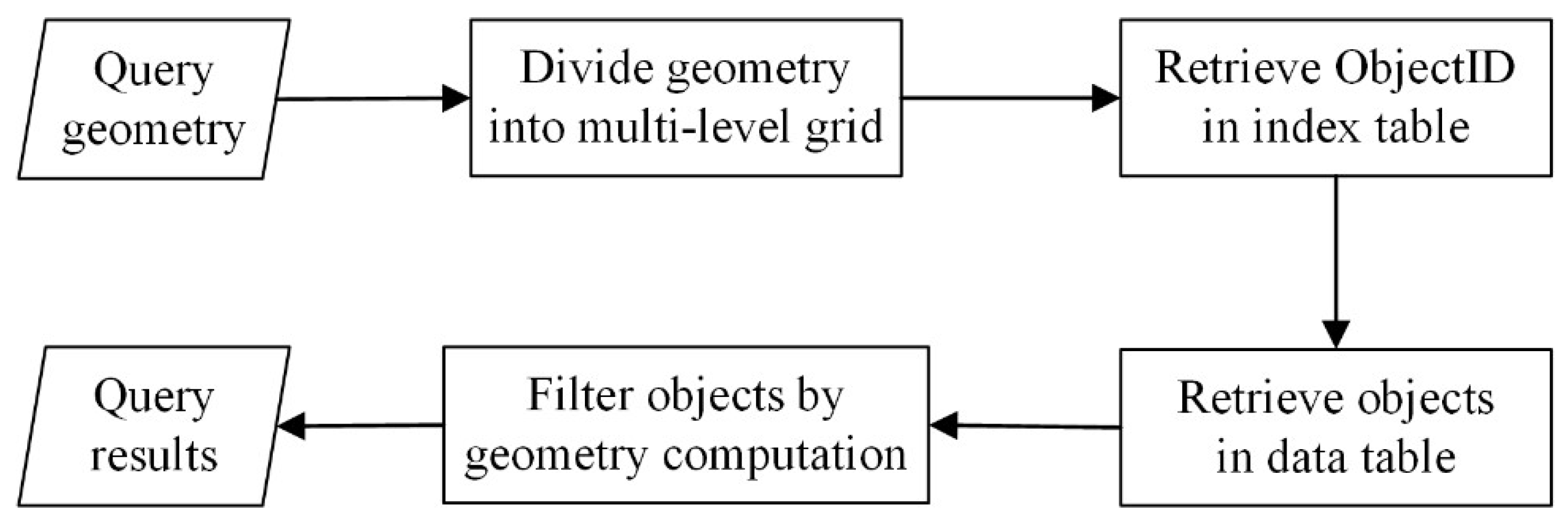
4. Vector Spatial Data Optimized Query

In this section, a new spatial index (Q-HBML) and two query optimization strategies are proposed to improve the efficiency of the spatial query. We first describe the Q-HBML index and a new algorithm for the generation of the hierarchical Hilbert code. The rowkey of the index table is also designed. Then, two query optimization strategies are analyzed. Furthermore, we apply our developed index and query optimization strategies for optimizing the topological query in HBase.

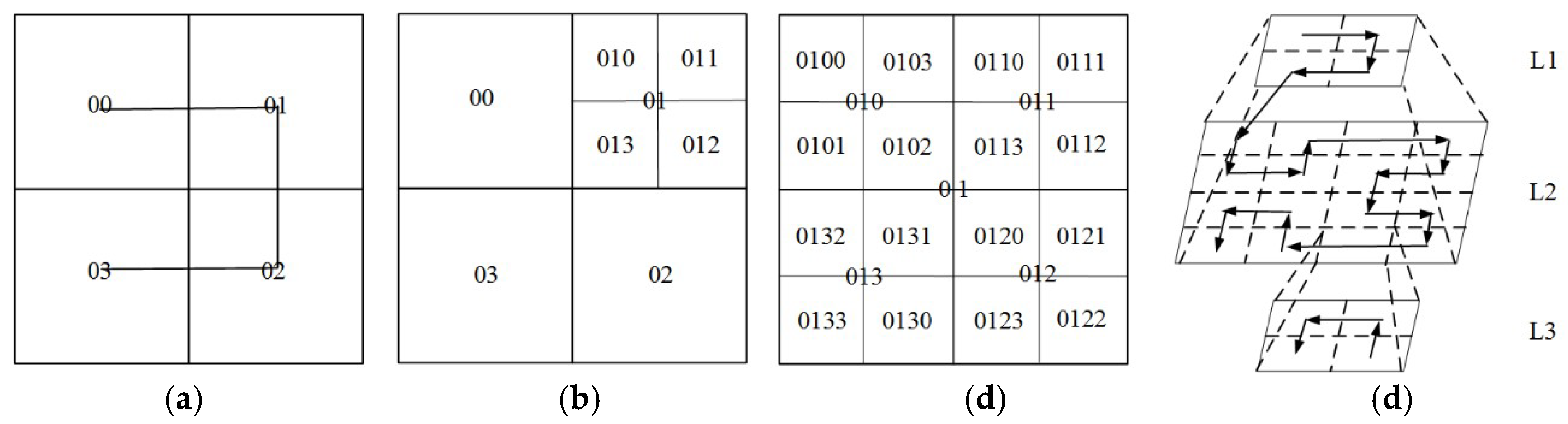
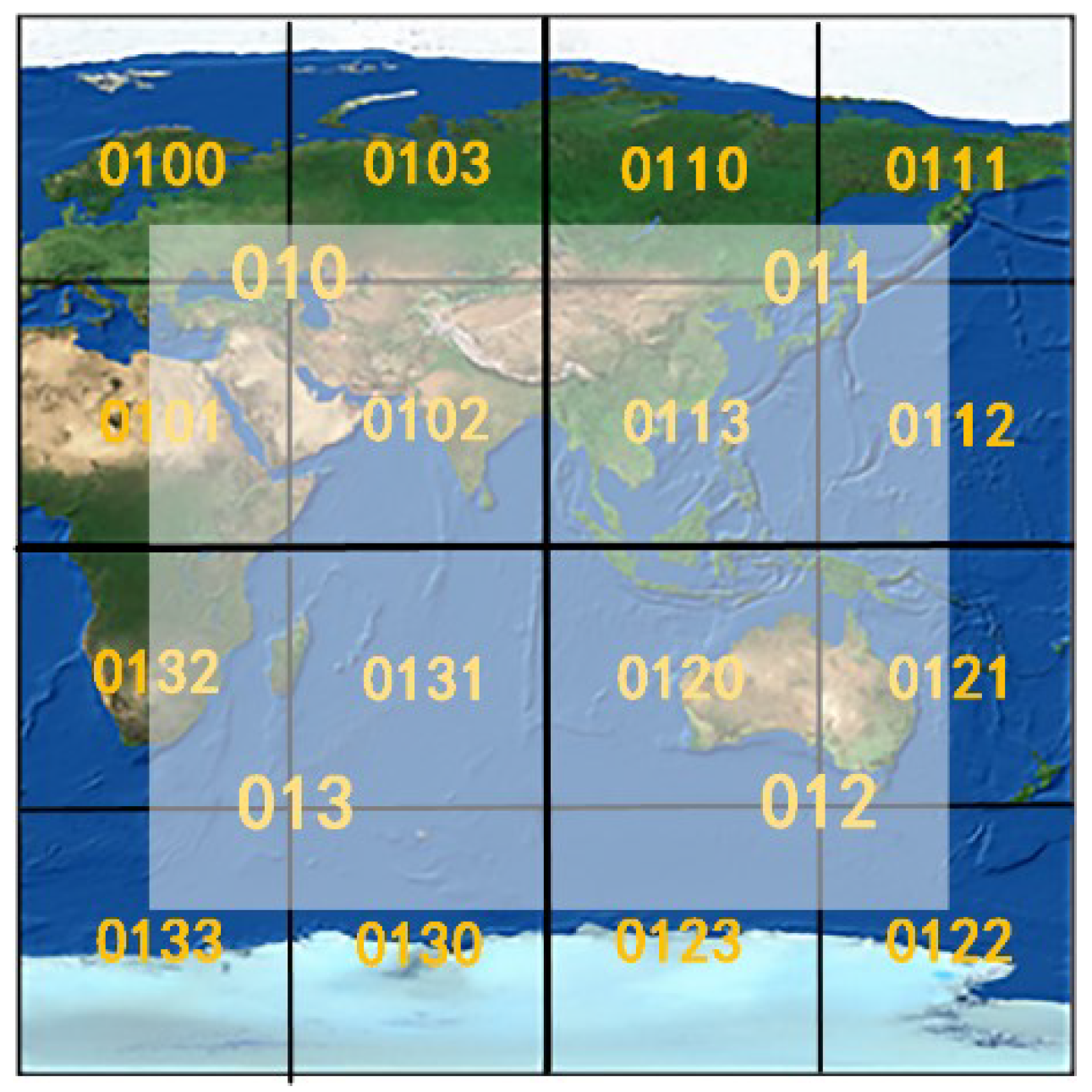
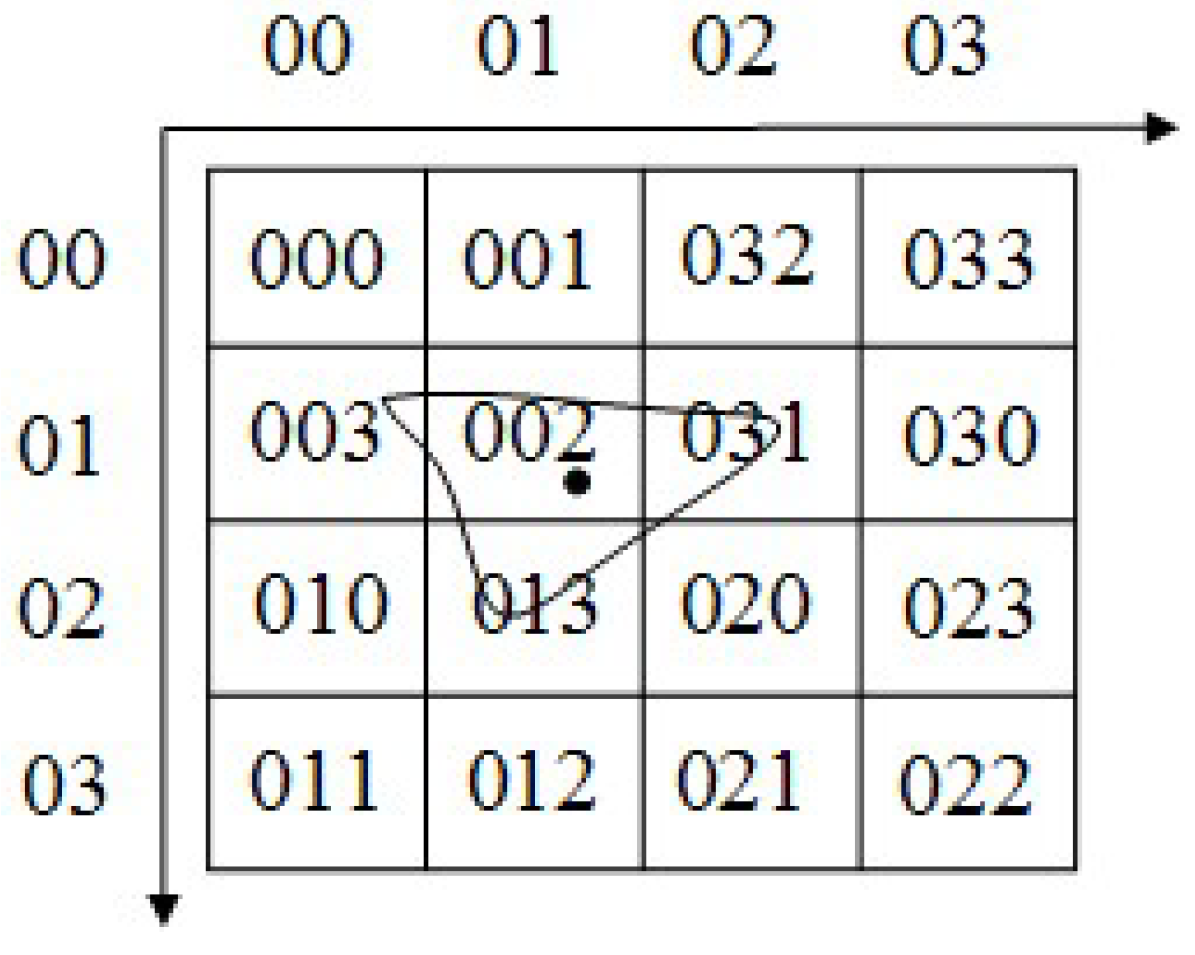
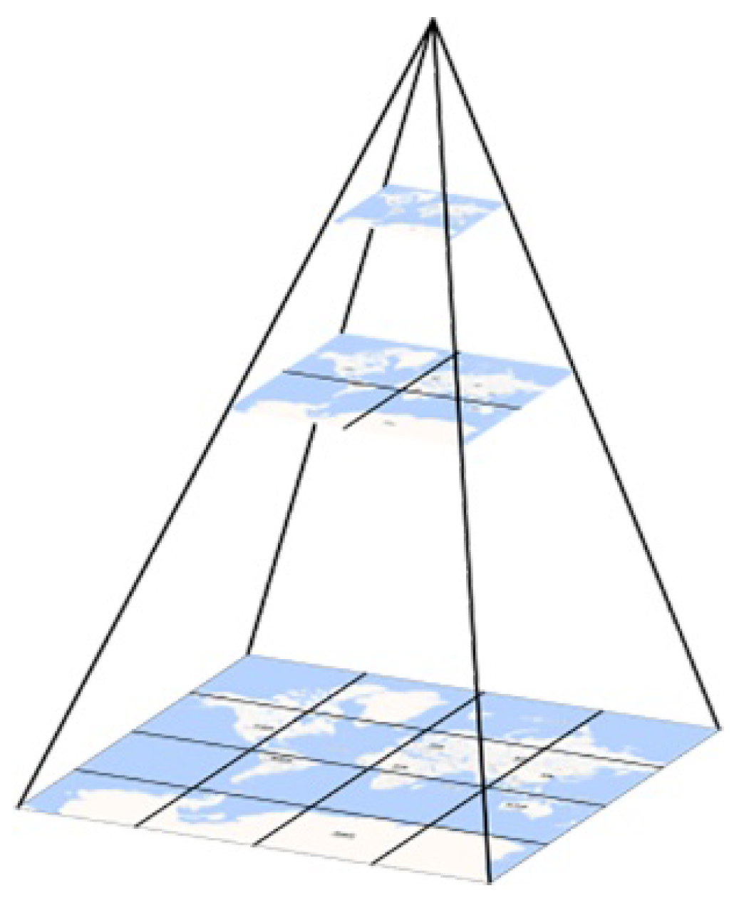
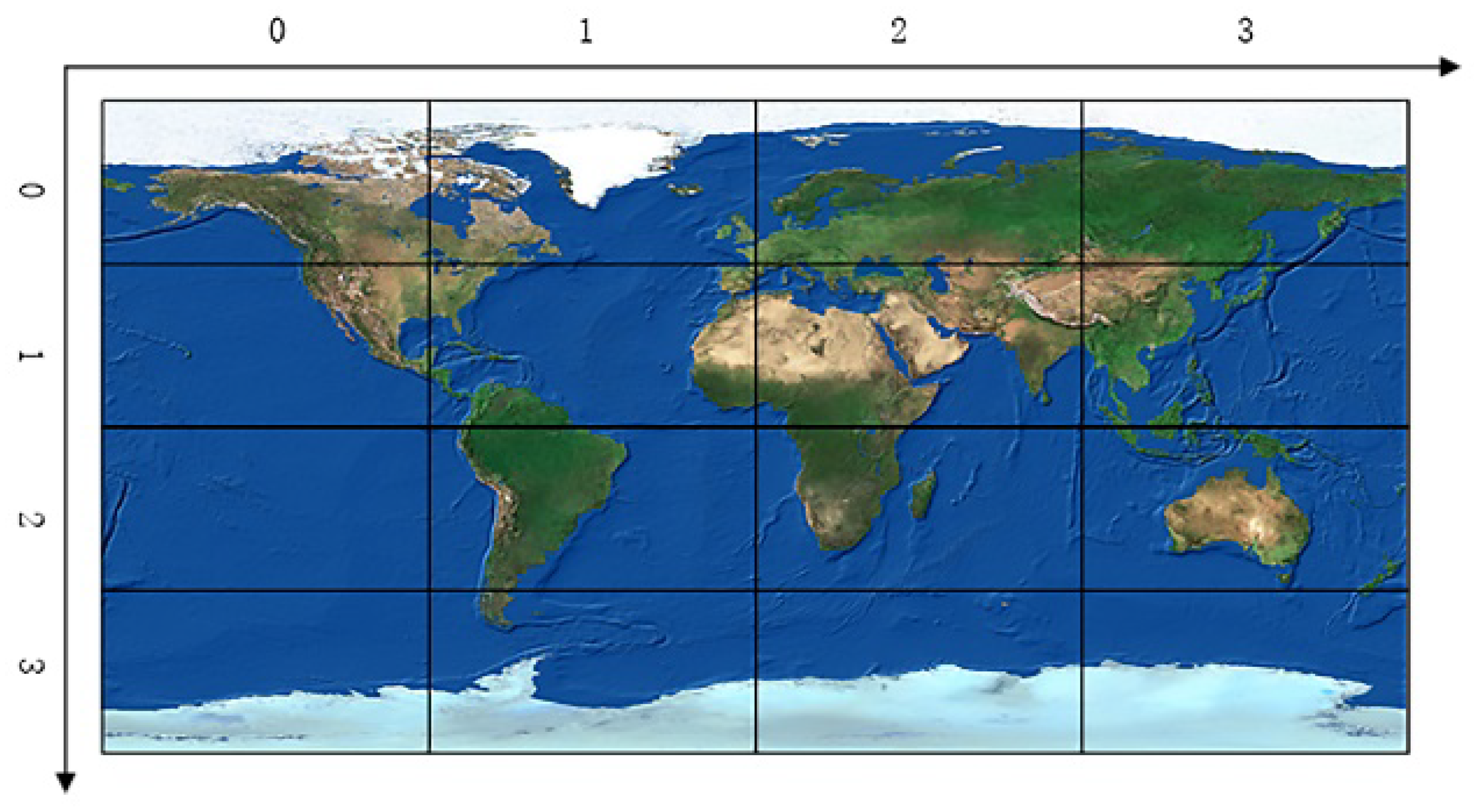
4.1. Quadtree-Hilbert-Based Multi-Level Grid Index

4.1.1. Algorithm of the Index

To build the Q-HBML index, first we use quadtree to divide the vector data into different rectangular levels, and the longitude-latitude grid is used to divide each quadtree level of the grids into a sequence of contiguous cells. After that, each cell in every level is encoded in hierarchical Hilbert codes. Finally, the rowkey of the spatial index table in HBase is designed.
The procedure of the Q-HBML partition is shown in Figure 2, and the grid begins to divide with the initial level; every grid cell in each level is regarded as a single unit. With the intersection of the Prime Meridian and the Equator as the central point, the size of the zero-level grid cell is 360° × 180°; the one-level is divided equally into four grid cells, each with a grid size of 180° × 90°. In each level, the longitude and latitude of every grid cell are transformed into the row and column (see Figure 3). By analogy, according to quadtree recursive subdivision, they form a multi-level grid of latitude and longitude. Then, we establish the mapping relationship between the different data scales and the corresponding levels.
When creating the Q-HBML index for vector polygon data, in addition to grid cells at the end level, the mapping relationships between a spatial object and the multi-level grid cells are only established for the grid cells completely overlaid by the MBR of the vector object. However, as long as the grid cells at the end level intersect with the MBR of a vector object, the mapping relationships of the grid cells to the spatial entity are also recorded. Therefore, there are two kinds of grid-object spatial relationships: partial coverage and coverage (see Figure 4).
Take an example: in Figure 4, the end level is L + 3, and a spatial object P is located in the grid cell (0,0) in the L level. P cannot be mapped into the grid cell (0,0) of level L as grid cell (0,0) has not been fully overlaid by the MBR of P. Thus, the grid cell divides into the next level L + 1. There are no grid cells at level L + 1 that are fully overlaid by the MBR of P. Then, the grid cells divide into the next level L + 2. In level L + 2, grid cells (1,1), (2,1) are fully overlaid by the MBR of P. Therefore, the mapping relationship between grid cells (1,1), (2,1) and P is established. Grid cells (1,1), (2,1) no longer split, and grid cells that are partly overlaid by the MBR of P need to further split into the next level. Because L + 3 is the end level, no other grid cells need to be divided.
Grid cells in Q-HBML are identified by the level number, row and column number. The Hilbert curve is applied to transform three-dimensional spatial data into a one-dimensional array and represent the encoding of grid cells. Most of the Hilbert curve works to encode grid cells in decimal format [15,24], such as 1, 2, 3, 12, 13. However, this kind of encoding is unable to represent the hierarchical relationship between grid cells at different levels, and it will cause a number of unrelated grid cells to access when scanning the Q-HBML index table in HBase. Consequently, based on the Hilbert curve algorithm proposed by Faloutsos and Roseman [15], this paper proposes a new algorithm (see algorithm1) for the generation of the Hilbert code and computes hierarchical Hilbert codes of grid cells to represent the hierarchical and neighborhood relationship between grid cells. This algorithm is shown as follows:
Algorithm 1. Generate hierarchical Hilbert codes of grid cells.
Input:r, c: row value and column value of a grid cell, l: level of the grid cell;
Output: h: hierarchical Hilbert code of the grid cell (r, c)
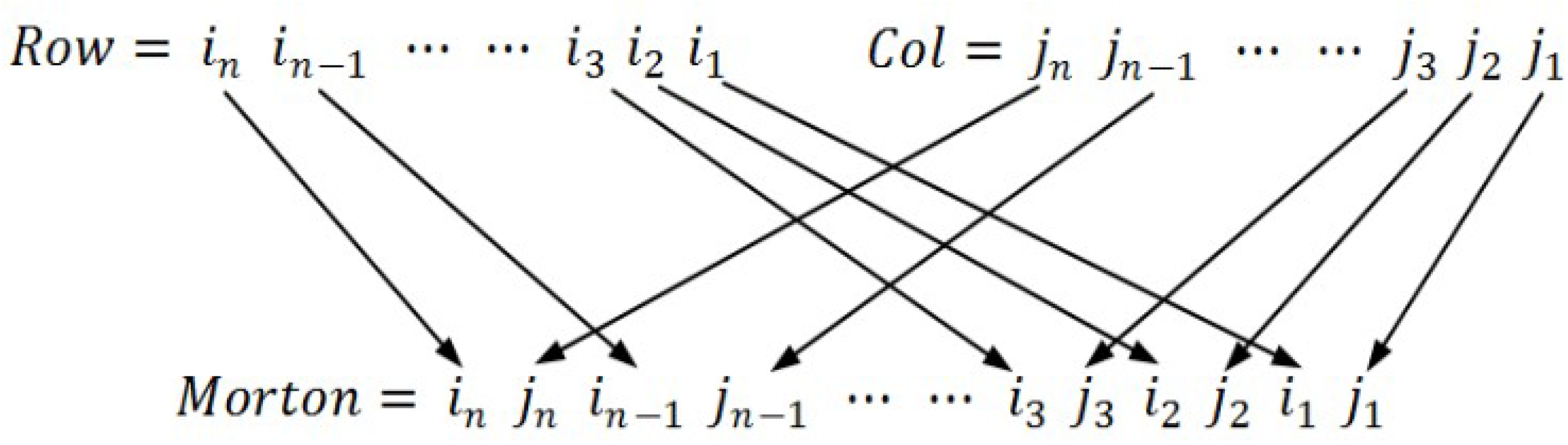
1. Step (1) transform r and c into L + 1-bit binary number, and then
2. turn it into the corresponding Morton code by interleaving bits of the two binary numbers (see Figure 5);
3. Step (2) divide the Morton code from left to right into 2-bit strings, and then
4. swap every ‘10’ and ‘11’;
5. Step (3) t i (i = 1, …, N) represents above every 2-bit string from left to right;
6. If t i = ‘00’, then
7. swap every following occurrence of ‘01’ and every following occurrence of ‘11’;
8. Else if t i = ‘11’, then
9. swap every following occurrence of ‘10’ and ‘00’;
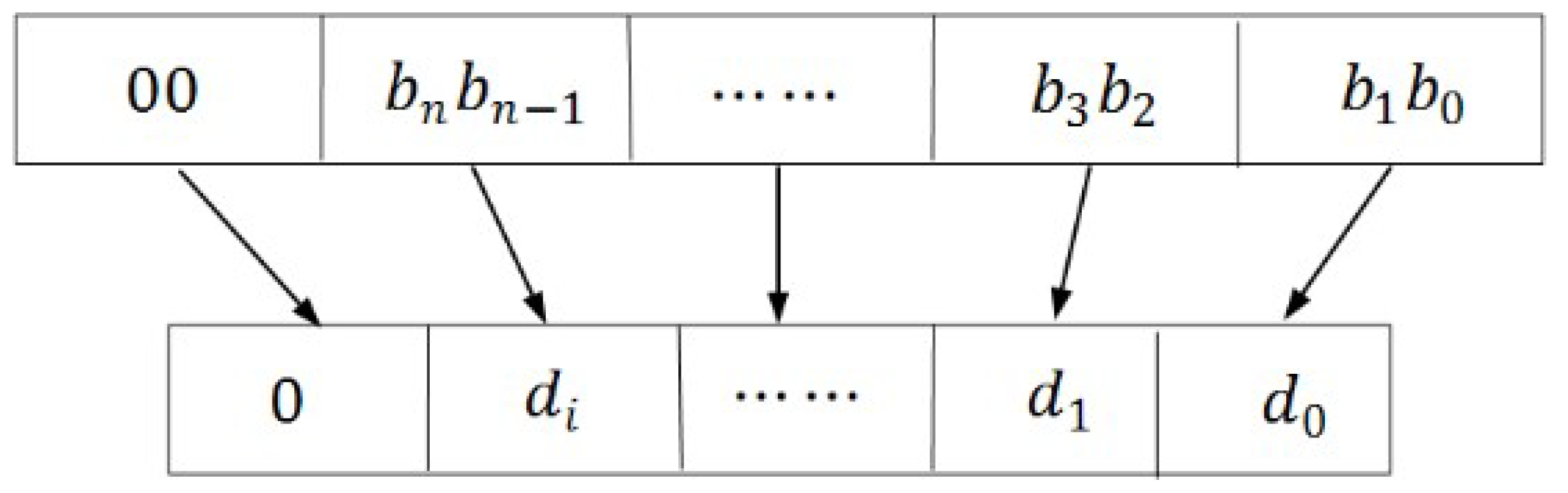
10. Step (4) from left to right, calculate the decimal values of each 2-bit string; see Figure 6;
11. Step (5) from left to right, concatenate all the decimal values in order and return the hierarchical
12. Hilbert code h; see Figure 7.
13. End
If we directly use the hierarchical Hilbert code as the rowkey of the index table, this design will result in vector data at the same level cross-storage after the internal index sort of HBase, and vector data at the same level that are adjacent in space cannot be represented closely (see Table 2). As shown in Figure 8 and Table 2, when we need to query vector data in the range of “010”, “011”, “012” and “013”, the pointer needs to move four times.
Therefore, this study designs the grid level number and hierarchical Hilbert code as the rowkey of the vector data index table to solve the above problems. Taking the grids of Level 3 as an example, Table 3 shows their storage schema in HBase; for the query area in Figure 8, the pointer only needs to move one time (move to “0100”).
Rowkey = grid level number + separator + hierarchical Hilbert code
The benefits of this index are as follows:
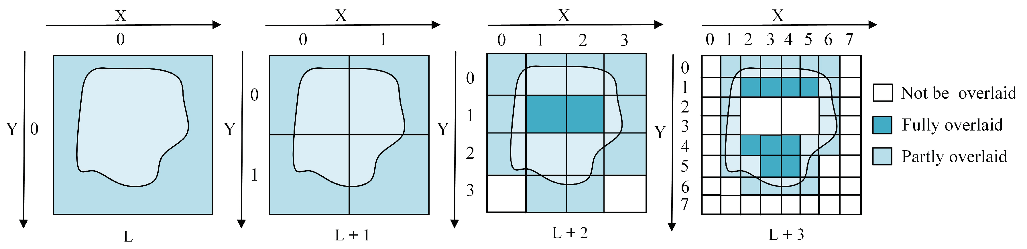
  • In the same grid level, the vector spatial data that are close in space are represented closely, which reduces the times of disk access, in particular for range query.
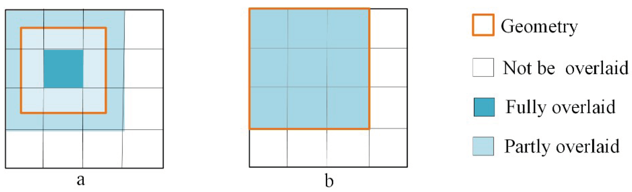
  • By using this Q-HBML grid index, we only need to further divide the grid cells that are partly overlaid by MBR of an object entity until reaching the end level, which reduces the grid cells’ redundant construction and improves the efficiency and precision of the spatial query.
  • The Hilbert code structure is relatively simple and highly scalable, and there is no need to pre-specify the code length. The length of the code can be dynamically expanded as the grid level increases.
  • The query operation is simpler. It is easy and quick to locate the query object indexes in the index table through the grid level and grid-object spatial relationships.

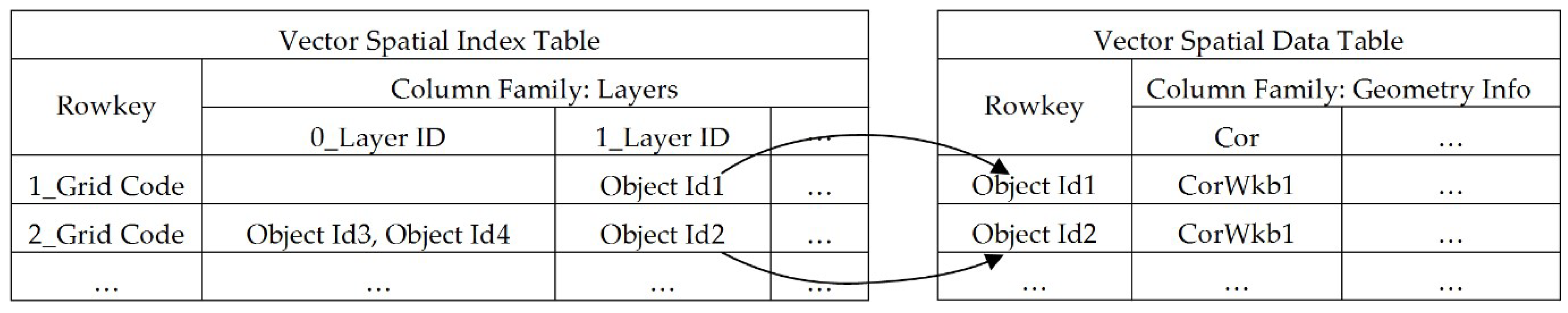
4.1.2. Index Table Architecture

As shown in Figure 9, we create an index table in the HBase database, which has a column family and develop the Q-HBML index codes for the vector object ranges. The rowkey of index table is designed in Section 4.1.1. The column has a value of zero or the ID of a plurality of vector entity records; each ID is the rowkey value of the corresponding spatial entity record in the vector spatial data table.
The design of the column name plays an important role in improving spatial query and filter efficiency. To identify the grid-object spatial relationships in columns, the column name is denoted as the concatenation of a spatial relationship code and a layer ID. For the spatial relationship code, the number “0” represents the partial coverage spatial relationship, and the number “1” represents the full coverage spatial relationship.
The advantage of the design of column names is conducive to greatly improving the spatial query efficiency. By analyzing the column name identifiers, the spatial relationship of the query objects can be preliminarily determined to filter too many unnecessary vector entities before taking complex spatial operations, improving spatial query performance. Besides, when there are only one or a few layers for spatial query, we can filter a large amount of unrelated index data by the layer ID in the column names.

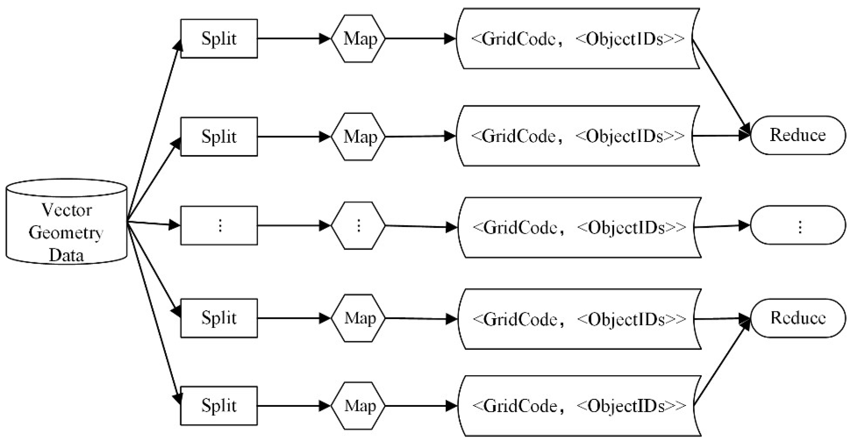
4.1.3. Index Parallel Construction

In fact, creating the spatial index for vector big data is a time-consuming process, especially when the grid level increases. This paper implements a method of creating the Q-HBML index in parallel based on MapReduce. The core idea of this method is described as follows (see Figure 10): After data partition provided by Hadoop, in the map stage, build the Q-HBML grid index for spatial entities on each layer, and export key/value pairs whose grid code is the key and the object ID codes mapped to spatial objects are the value. In the reduce stage, merge the output data in the map stage and write the index values to the index table.

4.2. Query Optimization Strategies

As shown in Figure 11, the flowchart of the spatial query is as follows: (1) first, divide the query geometry into multi-level grid cells in the Q-HBML index; (2) secondly, get the IDs of the target objects in the index table based on the grid-object spatial relationships between the vector objects and the query grid cells; (3) thirdly, obtain the object data in the data table through the object IDs; (4) finally, take the geometry computation for the obtained object data using GeoTools [25] to further filter useless objects, and then, get the final query results.
In the query processing, the two procedures of partitioning multi-level grids and scanning the index table perform important roles. Before determining which data buckets to scan, we must check index entries to determine if the grid cells corresponding to the entry intersect with the query. Spatial topological query involves different spatial relationship types, such as contain, overlap, etc. If we split the query geometry completely and check index entries that intersect with the query by scanning the index grid cells one by one for all spatial relationship types, this definitely increases the cost to scan the unnecessary grid cells. In essence, for the different query spatial relationship types, the ways to split the query geometry and scan index grid cells could be optimized. Based on the multi-level partition and spatial locality of the Q-HBML index in Section 4.1, this section proposes two corresponding new spatial query optimization strategies that eliminate a large number of unnecessary scans.
Through the research of the grid-object spatial relationships and spatial locality in the Q-HBML index, the following spatial query optimization strategies can reduce a large amount of scan operations, filtering a great deal of query data that do not match the spatial query conditions, thereby enhancing data query performance. The optimization strategies are as follows:
1. Optimized strategy on the spatial query operator
Apply different computation methods according to different spatial query operators, such as touch, contain, etc. Take the spatial relationship operation touch as an example: in the nine-intersection model [26], touch calculates the boundary of an object. The grid cells at the last level of the Q-HBML index constitute the boundary indexes of one object. The grid cells in the last level may be fully overlaid or partly overlaid by the query geometry (see Figure 12). Therefore, we can filter objects that are mapped by the fully-overlaid grid cells because it is impossible for these mapped objects to touch the query geometry. In the Q-HBML index, only the unique objects that are mapped by the partly-covered grid cells at the last level need to be selected to perform the touch geometry computation, instead of scanning all grid cells. Similarly, for other spatial query operators, such as contain, only the unique objects mapped by the grid cells at the last two levels need to be selected to perform the contain space computation. Because all grid cells of different levels except the final level are fully overlaid by the query geometry object in Q-HBML index, consequently, this strategy is able to reduce a large number of unnecessary scans and space computation, which greatly enhances the spatial query efficiency.
2. Optimized the strategy on merging grid cell codes
Merge continuous grid cell codes when scanning the index table to reduce the numbers of scans. Generally, when scanning continuously hundreds of grid cells, the grid cells will be scanned one by one in HBase, which seriously reduces the query efficiency. However, grid cell codes in the Q-HBML index table are first sorted by level and then sorted by hierarchical Hilbert codes. Thus, the method of merging continuous scan grid cells in each level by the start grid cell and the end grid cell is an effective way to reduce the number of scans and improve query efficiency.

4.3. Optimized Topological Query

According to the above spatial optimization strategies, a Q-HBML-based optimized topological query algorithm (see Algorithm 2), ML-OTQ, is proposed. There are two core ideas in the process of the topological optimized query: (a) it first determines the effective and efficient computation methods according to different topological query relationships and then further filters unrelated objects based on the grid-object spatial relationships before performing the geometry computation; and (b) merges continuous grid cell codes to reduce the number of scans. The main steps of this algorithm are as follows.
Algorithm 2. Topology optimized query.
Input: g: spatial query geometry; l i s : start level in index table, l i e : end level in index table, r: query topological relationship type;
Output: S: array of vector spatial data;
1. Step (1) l g s Calculate the start level of g by CalculatePartitionStartLevel (see Algorithm 3);
2. Step (2) if l g s > l i s , then
3.  C 0 Calculate the grid cells where the center point of g is located from l i s to l g s ;
4. otherwise, next;
5. Step (3) grid cells at the level l i e -1 C e 1 , grid cells at the level l i e   C e Calculate the multi-level
6. grids mapping of g from the level l i s to the level l i e , then next;
7. Step (4) Determine the computation methods according to the topological relationship r.
8. If r is one of contain, within, intersect, equal and overlap, then
9. enter the next step;
10. else if r is one of cross, touch and disjoint, then
11. skip to Step (7);
12. Step (5) Merge all continuous grid cell codes at the levels l i e -1 and l i e
13.  M C 0 Merge C 0 ,
14.  M C e 1 Merge C e 1 ,
15.  M C e Merge C e , then next;
16. Step (6) Scan the index table by the grid-object spatial relations, and get corresponding unique
17. vector IDs
18.  V 0 Scan index table for M C 0 , and get corresponding index values through r,
19.  V e 1 Scan index table filter unrelated index values by the grid-object spatial
20. relations for M C e 1 , and get corresponding index values through r,
21.  V e Scan index table filter unrelated index values by the grid-object spatial
22. relations for M C e , and get corresponding index values through r,
23.  V V 0 V e 1 V e , then skip to Step 9;
24. Step (7) Merge all continuous grid cell codes at the level l i e
25.  M C 0 Merge C 0 ,
26.  M C e Merge C e , then next;
27. Step (8) Scan index table by the grid-object spatial relations, and get corresponding unique
28. vector IDs
29.  V 0 Scan index table for M C 0 , and get corresponding index values through r,
30.  V e Scan index table and filter unrelated index values by the grid-object spatial
31. relations for M C e through r,
32.  V V 0 V e , then next;
34. Step (9) S Take geometry operations for V according to r, filter useless objects, and get
35. results.
36. return S
37. End.
Algorithm 3. Calculate the start level of the partition.
Input:g: spatial query geometry;
Output: l g s : the start partition level of g
1.  M Compute the MBR of g;
2.  L w Compute the largest level in the Q-HBML index whose grid size contains the width of M ;
3.  L l Compute the largest level in the Q-HBML index whose grid size contains the length of M ;
4. If L l L w , then
5. return L w ;
6. else
7. return L l ;
8. End.

5. Evaluation

In this section, experiments are evaluated based on the real-world dataset. The environment of the experiments is introduced in Section 5.1. Section 5.2 gives the details of our experimental data. Section 5.3 shows the performance of horizontal HBase cluster expansion. Section 5.4 describes the Q-HBML index experiments. Spatial query optimization strategy experiments are described in Section 5.5. Finally, Section 5.6 shows the comparison of PostGIS, the regular grid index built on HBase, GeoMesa built on HBase and GeoWave built on HBase.

5.1. Experimental Environment

In this experiment, the cloud computing cluster is provided by several servers. The details of their configuration are shown in Table 4. Besides, a server is used as the test machine. Table 5 shows the configuration of the test machine. In the experiment, query response time is counted five times to obtain the average. We implemented the range query processing with the coprocessor framework, considering the relatively large queried range.

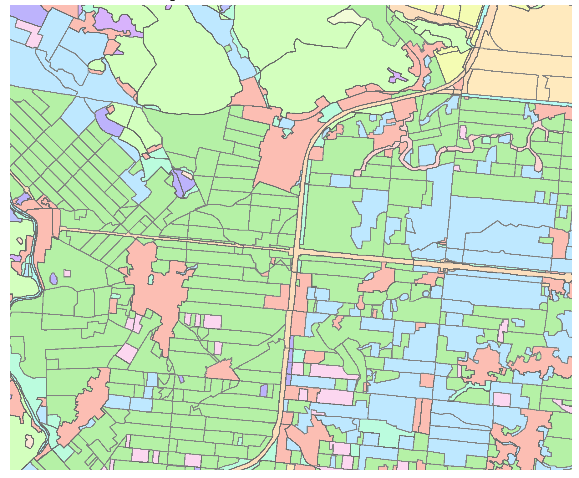
5.2. Experimental Data

In our experiment, spatial data are a map delineation set of land for land use in Hangzhou city (including 13 administrative districts). There are 6,782,561 polygons in the dataset. The whole data size is about 12.55 G. The record number of Jihong village is 113,625. The record number of Sandun town is 201,367. The record number of Hangzhou downtown is 2,102,648. A part of geographic area in Hangzhou downtown is shown in Figure 13.

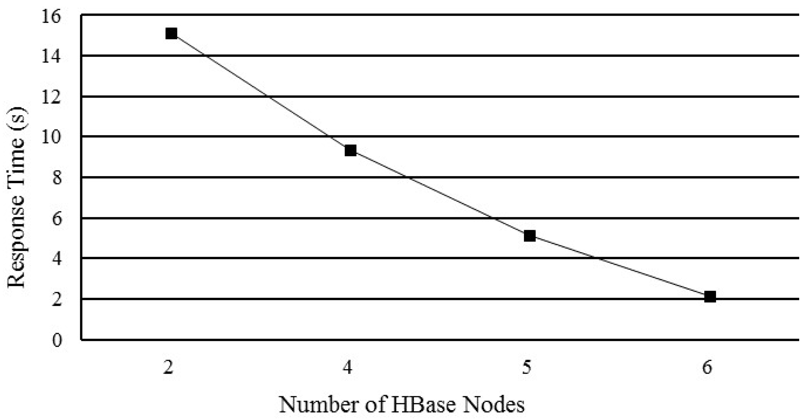
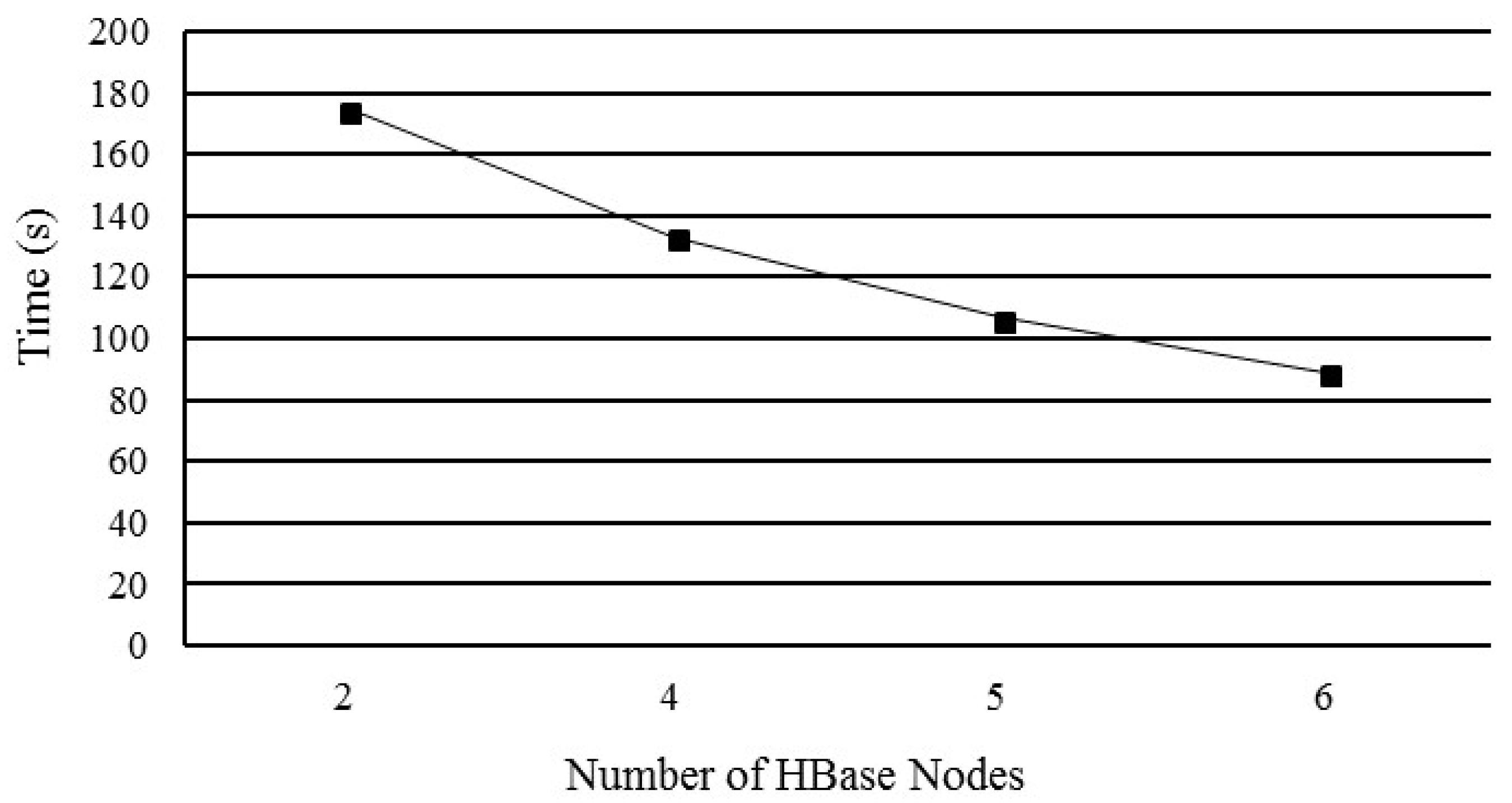
5.3. Performance of Horizontal HBase Cluster Expansion

In this section, the scalability performances of creating index and region query are validated. This experiment creates the Q-HBML index of the test dataset (6,782,561 polygons) by different numbers of HBase nodes. The start level of the index is 10, and the end level is 16. The result of creating index is shown in Figure 14. With the increase of the number of HBase nodes, the time of creating the index of vector spatial data is decreasing; because the MapReduce model can make use of multiple server nodes to create the index in parallel.
An experiment is also conducted to test the time of the range query by different numbers of HBase nodes. A rectangles area (118.607, 29.199, 119.344, 30.176) is chosen as the query region, which contains about 969,514 polygons. Figure 15 reports the response time of the range query with different numbers of HBase nodes. It is obvious that horizontal cluster expansion can improve spatial query efficiency and demonstrate the scalability of the index.
Therefore, the following experiments are performed on a six-node cluster. One of them is the master, acting as the name node, job tracker and HMaster. The other nodes are slave nodes, acting as the data node, compute node, task tracker and HRegionServer.

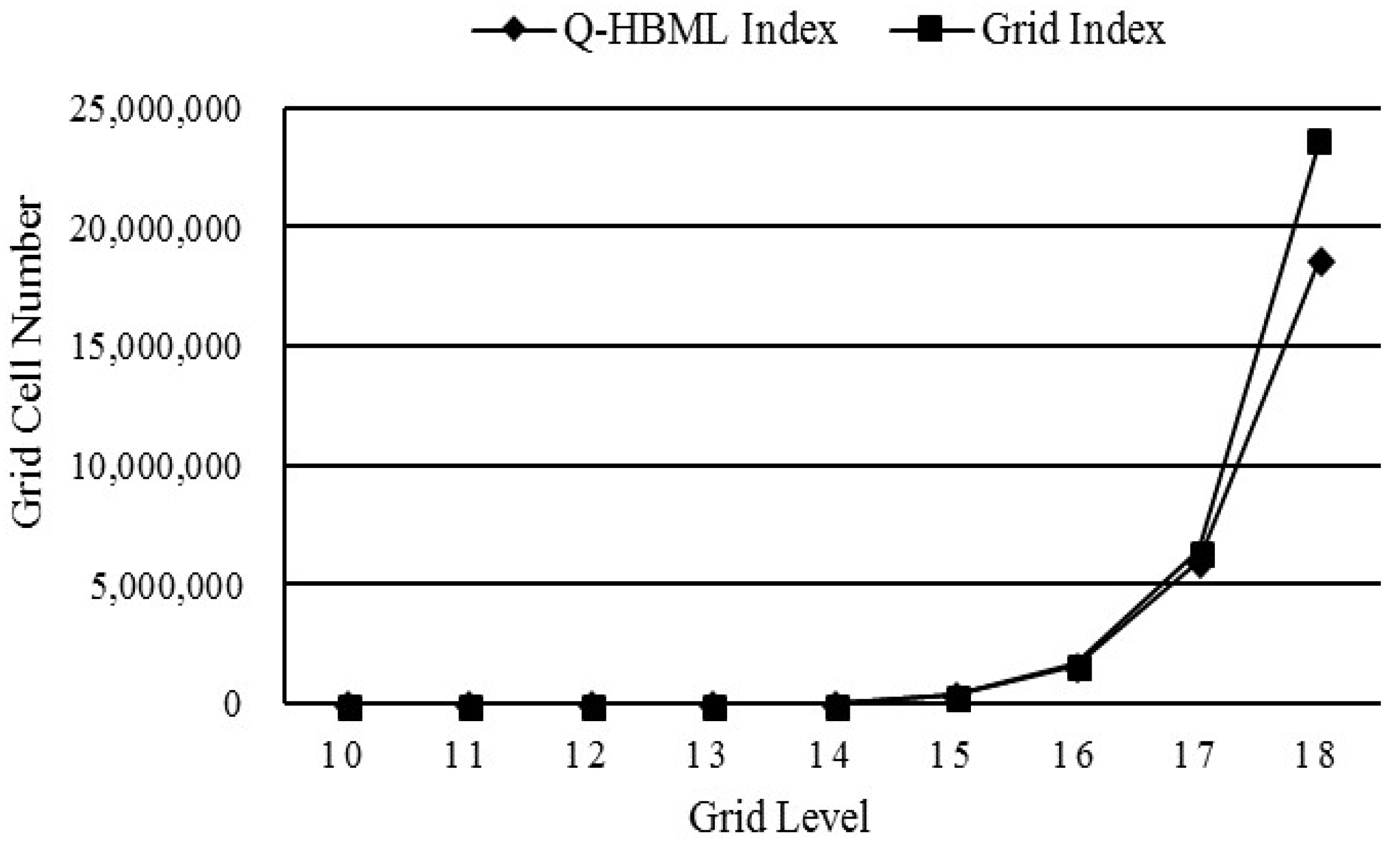
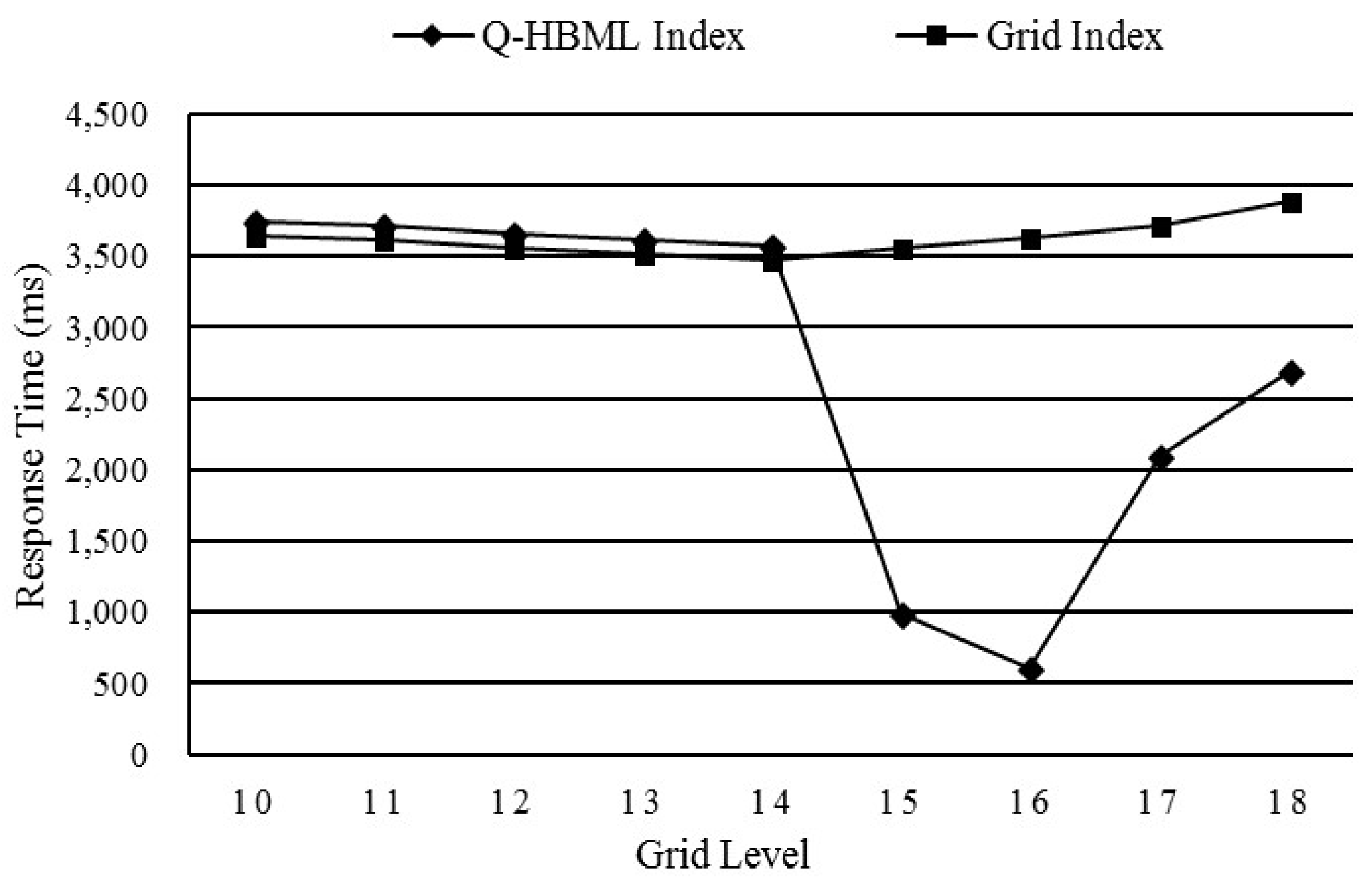
5.4. Comparison of the Q-HBML Index and the Regular Grid Index

To validate the effectiveness of the Q-HBML index proposed in this paper, experiments are designed to evaluate the grid cell construction number and region query efficiency in the dataset. In the experiments, with grid levels from 10–18, grid construction is executed in the Q-HBML index and traditional regular grid index, separately. Then, in the geographical region (118.904, 29.634, 119.139, 29.863), region queries are also executed separately in the Q-HBML index and traditional regular grid index.
Results on the grid cell construction number and query response time of the two indexes are shown in Figure 16 and Figure 17. It can be seen from them that, when the grid level is between 10 and 14, the number of grid cells constructed by the Q-HBML index and grid index is the same, and the query response time of the Q-HBML index and grid index is also almost the same. Nevertheless, when the grid size is gradually refined, as starting from Grid Level 17, the number of grid cells constructed by the Q-HBML index is obviously smaller than that of the grid index. Meanwhile, the response time of the Q-HBML index is quite lower than that of the grid index.
Compared with the grid index, results indicate that the Q-HBML index can reduce the redundancy of grid cells and has better query efficiency. From the 10th level to the 14th level, all grid cells contain the largest MBR of vector entities. That is why both indexes have the same grid cell construction numbers between the 10th and 14th level. However, from the 15th level to the 18th level, the number of grid cells constructed by the Q-HBML index is obviously smaller than that of the grid index. This is because, in the Q-HBML index, the grids do not need to split further if these grid cells are overlaid by the MBR of a vector entity, which reduces the redundancy of grid cells. The number of grid cells is an important factor that affects the efficiency of the spatial query. Therefore, as shown in Figure 17, the query response time of the Q-HBML index is lower than that of grid index from the 15th level to the 18th level because of the smaller number of grid cells constructed by the Q-HBML index. However, with the increase of the grid level between the 16th and 18th, the query efficiency of the Q-HBML index decreases. The reason is that a larger number of grid cells needs to be scanned and takes up more space. Therefore, an optimal grid level value for the Q-HBML index is the 16th level in this dataset. Besides, the design of the rowkey in the Q-HBML index also contributes to the higher query efficiency because it makes the spatial indexes of entities that are close in distance be able to be stored close together on disks and reduces the scan time.

5.5. Performance of the Spatial Query Optimization Strategy

After the last experiments, the experiments in this subsection were designed to validate the effectiveness of the spatial query optimization strategies for the different sizes of spatial query objects. In our experiments, three different levels of administrative districts, including the rural area, town and urban area, were chosen as geographical regions for the spatial query. The record number of urban area data is larger than that of town area data, and the record number of town area data is larger than that of rural area data. Based on the Q-HBML index, the following optimization strategy tests were designed for the optimized strategy on the spatial query operator and the optimized strategy on the merging grid cell codes.

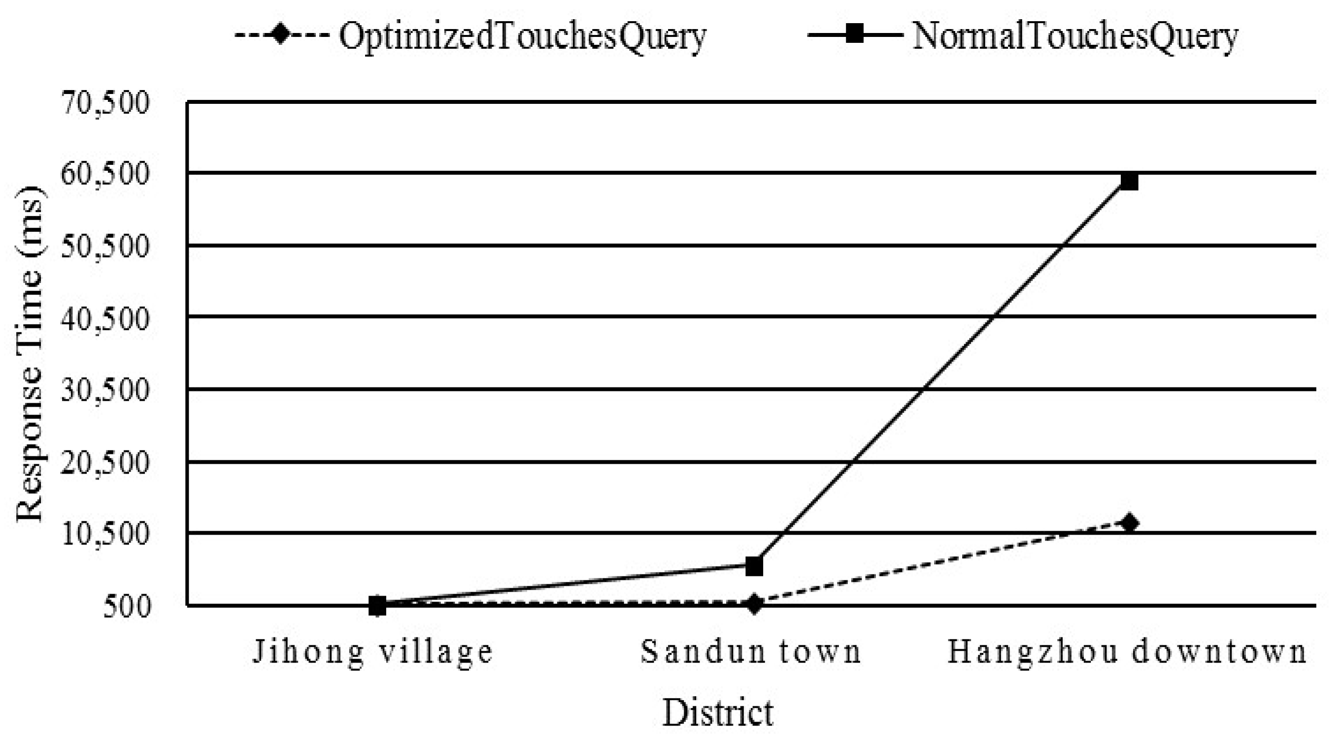
5.5.1. Test 1: Influence of the Optimized Strategy on the Spatial Query Operator

The result of the response time of the touch spatial query with the optimized strategy on the spatial query operator is shown in Figure 18. We can conclude that the efficiency of the former is better than the latter, especially for more data records to query, such as the difference of the response time of queries in Hangzhou downtown.
Actually, the efficiency of the touch spatial query depends on the record number that needs to be operated. As we can see in Section 4.2, for the optimized strategy on the touch query, only the unique objects that are mapped by partly-covered grid cells at the last level need to be selected for touch geometry computation. In contrast, for the normal touch query, when querying the index table, not only are vector entities that touch the query target obtained, but also some vector entities that intersect with or are contained by the query target are, as well.

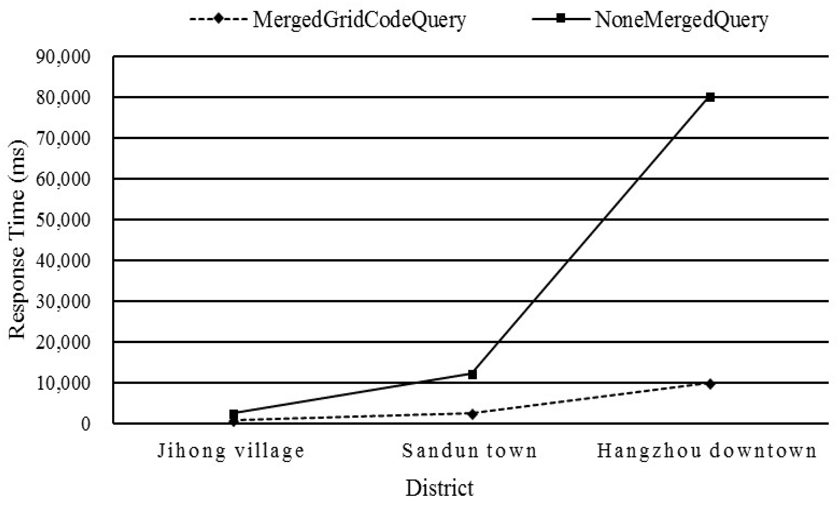
5.5.2. Test 2: Influence of the Optimized Strategy on the Merging Grid Cell Codes

The result on the response time of the intersection spatial query with the optimized strategy on the merging grid cell codes is shown in Figure 19. From Jihong village to Hangzhou downtown, it is obvious that the efficiency of the former is increasingly better than the latter as the query records grow.
Actually, the optimized strategy on merging grid cell codes is based on the clustering storage of rowkeys of the index table on disks. For the optimized strategy on merging grid cell codes, the continued grid cells that are close in space will be merged. Therefore, when scanning the index table in HBase, only the merged grid cells will be scanned. However, for the normal query that does not merge grid cells, all grid cells will be scanned one by one, which definitely reduces the spatial query efficiency.

5.6. Comparison of PostGIS, Regular Grid Index, GeoMesa and GeoWave

In this section, we compare the performance of PostGIS, the regular grid index, GeoMesa and GeoWave with range queries. The regular grid index, GeoMesa and GeoWave are built on HBase. We set the appropriate grid level to 16 as the end level for our Q-HBML and regular grid index. In the experiment, ten chosen rectangular areas are used for region query and are shown in Table 6. The following measurements were separated by the first iteration, in which no results were present in the cache yet. The result on query response time of these methods is shown in Table 7.
From Table 7, we can see that PostGIS is slightly better than the others for the small queries, while our method, GeoWave and GeoMesa outperform the others for the large queries. With the scale growth of data, the query times of PostGIS grow rapidly and continuously, followed by the regular grid index. The query times of our method, GeoWave and GeoMesa grow steadily.
In the experiment, the performance comparison between PostGIS and the other distributed storage methods in HBase proves that HBase is suitable for vector big data storage. Compared with the regular grid index, our method performs much better, especially when the amount of data increases. This is because, for our method, we can quickly locate the grid cells without scanning the full table by the design of the rowkey and Q-HBML index, and the query optimization mechanisms offer better pruning of unrelated data and fewer false positives, which greatly improve the performance of the query.
Comparing our method, GeoMesa and GeoWave, for the smaller region queries of the polygon data, the query efficiency of our method is similar to that of GeoMesa and GeoWave, while our method performs slightly better than GeoMesa and slightly worse than GeoWave for the larger queries. One of the reasons may be that GeoMesa uses the XZ curve for data with spatial extent, while our method and GeoWave use the Hilbert curve to represent two-dimensional grids at multiple levels. The Hilbert curve preserves a better locality than the Z-curve [27]. As the query region grows, more irrelevant data have to be scanned, since the Z-curve for ordering cells does not keep a good locality among subspaces. Another reason could be that our method just scans grid cells at the last two levels for region query and further filters many unrelated grid cells through the coverage and partial coverage relationships before making the geometry computation, which significantly reduces the time greatly.
Overall, our method demonstrates its query strength for polygon data when it comes to larger amounts of data.

6. Conclusions

This paper focuses on the storage schema and fast topological query of massive vector polygon data in HBase. A quadtree and Hilbert-based multi-level grid index and two query optimization strategies are proposed. Firstly, in the vector data storage model, we design the HBase storage format, and the rowkey in HBase table is the concatenation of the Hilbert value of grid cells to which the center of the object entity’s MBR belongs, the layer identifier and the order code. Secondly, a multi-level grid index structure, Q-HBML, is designed, and a generic algorithm for the Hilbert code is put forward to encode hierarchical Q-HBML grid cells. The rowkey in the index table is the concatenation of the grid level number and the hierarchical Hilbert code. Then, two query optimization strategies are proposed to optimize the spatial query process. Finally, based on the Q-HBML index and query optimization strategies, an optimized topological query algorithm is presented to improve the topological query efficiency.
Four groups of experiments are designed to validate the efficiency of our method. Experiments demonstrate that the Q-HBML index has high scalability, less grid redundancy and better topological query efficiency, and query optimization strategies can enhance the access efficiency. It is also proven that the range query efficiency of our method obviously outperforms PostGIS and the regular grid index for vector polygon big data.
In our study, although the query efficiency of vector data has been improved, the space of index storage and the performance of spatial relationship parallel computation can be optimized further. These will be discussed in future work.

Author Contributions

H.J., J.K. and Z.D. conceived of and designed the experiments. H.J. and F.Z. performed the experiments. H.J., X.H. and R.L. analyzed the data. X.Z. contributed data. H.J. wrote the paper.

Acknowledgments

This work was supported by the National Natural Science Foundation of China (Grant Nos. 41471313, 41101356, 41671391), the National Key Research and Development Program of China (Grant No. 2016YFC0803105), the Natural Science Foundation of Jiangxi (Grant No 20142BBE50024), the Science and Technology Project of Zhejiang Province (Grant Nos. 2014C33G20 and 2013C33051), the Jiangxi Provincial Department of Education Science and Technology Research Projects (Grant Nos. 3204704062 and 3204704061) and the Major Program of China High Resolution Earth Observation System (Grant No. 07-Y30B10-9001).

Conflicts of Interest

The authors declare no conflict of interest.

References

  1. Wang, Y.; Li, C.; Li, M.; Liu, Z. Hbase Storage Schemas for Massive Spatial Vector Data. Clust. Comput. 2017, 20, 1–10. [Google Scholar] [CrossRef]
  2. Zhang, N.; Zheng, G.; Chen, H.; Chen, J.; Chen, X. Hbasespatial: a Scalable Spatial Data Storage Based on Hbase. In Proceedings of the 2014 IEEE 13th International Conference on Trust, Security and Privacy in Computing and Communications, Beijing, China, 24–26 September 2014; pp. 644–651. [Google Scholar]
  3. Wang, L.; Chen, B.; Liu, Y. Distributed Storage and Index of Vector Spatial Data Based on Hbase. In Proceedings of the 21st International Conference on Geoinformatics, Kaifeng, China, 20–22 June 2013; pp. 1–5. [Google Scholar]
  4. Nishimura, S.; Das, S.; Agrawal, D.; El Abbadi, A. MD-Hbase: Design and Implementation of an Elastic Data Infrastructure for Cloud-Scale Location Services. Distrib. Parallel Databases 2013, 31, 289–319. [Google Scholar] [CrossRef]
  5. Chang, F.; Dean, J.; Ghemawat, S.; Hsieh, W.C.; Wallach, D.A.; Burrows, M.; Chandra, T.; Fikes, A.; Gruber, R.E. Bigtable: A distributed storage system for structured data. In Proceedings of the 7th USENIX Symposium On Operating Systems Design And Implementation—Volume 7, Seattle, WA, USA, 6–8 November 2006; USENIX Association: Berkeley, CA, USA, 2006; p. 15. [Google Scholar]
  6. Apache Phoenix. Available online: http://Phoenix.Apache.Org/ (accessed on 14 March 2018).
  7. Han, D.; Stroulia, E. Hgrid: A Data Model for Large Geospatial Data Sets In Hbase. In Proceedings of the 2013 IEEE Sixth International Conference on Cloud Computing, Santa Clara, CA, USA, 28 June–3 July 2013; pp. 910–917. [Google Scholar]
  8. Guttman, A. R-Trees: A Dynamic Index Structure for Spatial Searching. In Proceedings of the 1984 ACM SIGMOD International Conference on Management of Data, Boston, MA, USA, 18–21 June 1984; pp. 47–57. [Google Scholar]
  9. Sharifzadeh, M.; Shahabi, C. Vor-Tree: R-Trees with Voronoi Diagrams for Efficient Processing of Spatial Nearest Neighbor Queries. Proc. VLDB Endow. 2010, 3, 1231–1242. [Google Scholar] [CrossRef]
  10. Dutton, G. Improving Locational Specificity of Map Data—A Multi-Resolution, Metadata-Driven Approach And Notation. Int. J. Geogr. Inf. Syst. 1996, 10, 253–268. [Google Scholar]
  11. Nievergelt, J.; Hinterberger, H.; Sevcik, K.C. The Grid File: An Adaptable, Symmetric Multikey File Structure. ACM Trans. Database Syst. 1984, 9, 38–71. [Google Scholar] [CrossRef]
  12. Finkel, R.A.; Bentley, J.L. Quad Trees A Data Structure for Retrieval On Composite Keys. Acta Inform. 1974, 4, 1–9. [Google Scholar] [CrossRef]
  13. Zhou, Y.; Zhu, Q.; Zhang, Y. GIS Spatial Data Partitioning Method for Distributed Data Processing. In International Symposium on Multispectral Image Processing and Pattern Recognition; SPIE: Wuhan, China, 2007; Volume 6790, pp. 1–7. [Google Scholar]
  14. Wang, Y.; Hong, X.; Meng, L.; Zhao, C. Applying Hilbert Spatial Ordering Code to Partition Massive Spatial Data In PC Cluster System. In Geoinformatics 2006: GNSS And Integrated Geospatial Applications; SPIE: Wuhan, China, 2006; Volume 642, pp. 1–7. [Google Scholar]
  15. Faloutsos, C.; Roseman, S. Fractals for Secondary Key Retrieval. In Proceedings of the Eighth ACM SIGACT-SIGMOD-SIGART Symposium on Principles of Database Systems; ACM: Philadelphia, PA, USA, 1989; pp. 247–252. [Google Scholar]
  16. Shaffer, C.A.; Samet, H.; Nelson, R.C. Quilt: A Geographic Information System Based on Quadtrees. Int. J. Geogr. Inf. Syst. 1990, 4, 103–131. [Google Scholar] [CrossRef]
  17. Li, G.; Li, L. A Hybrid Structure of Spatial Index Based on Multi-Grid And QR-Tree. In Proceedings of the Third International Symposium on Computer Science and Computational Technology, Jiaozuo, China, 14–15 August 2010; pp. 447–450. [Google Scholar]
  18. Geomesa. Available online: http://www.Geomesa.Org/ (accessed on 12 April 2018).
  19. Böxhm, C.; Klump, G.; Kriegel, H. XZ-Ordering: A Space-Filling Curve for Objects with Spatial Extension. In Advances in Spatial Databases; Springer: Berlin/Heidelberg, Germany, 1999. [Google Scholar]
  20. Geowave. Available online: https://Github.Com/Locationtech/Geowave (accessed on 12 April 2018).
  21. Elasticsearch. Available online: https://www.Elastic.Co (accessed on 12 April 2018).
  22. Hulbert, A.; Kunicki, T.; Hughes, J.N.; Fox, A.D.; Eichelberger, C.N. An Experimental Study of Big Spatial Data Systems. In Proceedings of the IEEE International Conference On Big Data (Big Data), Washington, DC, USA, 5–8 December 2016; pp. 2664–2671. [Google Scholar]
  23. Dimiduk, N.; Khurana, A.; Ryan, M.H.; Stack, M. Hbase in Action; Manning Shelter Island: Shelter Island, NY, USA, 2013. [Google Scholar]
  24. Tak, S.; Cockburn, A. Enhanced Spatial Stability with Hilbert And Moore Treemaps. IEEE Trans. Vis. Comput. Graph. 2013, 19, 141–148. [Google Scholar] [CrossRef] [PubMed]
  25. Geotools. Available online: http://Geotools.Org/ (accessed on 12 April 2018).
  26. Egenhofer, M.; Herring, J. A Mathematical Framework for the Definition of Topological Relationships. In Proceedings of the Fourth International Symposium On Spatial Data Handling, Zurich, Switzerland, 23–27 July 1990; pp. 803–813. [Google Scholar]
  27. Haverkort, H.; Walderveen, F. Locality and Bounding-Box Quality of Two-Dimensional Space-Filling Curves. In Proceedings of the 16th Annual European Symposium on Algorithms; Springer: Karlsruhe, Germany, 2008; pp. 515–527. [Google Scholar]
Figure 1. Spatial entity division.
Information 09 00116 g001
Figure 2. Q-HBML grids’ partition.
Information 09 00116 g002
Figure 3. Grid cells ‘representation.
Information 09 00116 g003
Figure 4. Instance of multi-level grid vector object segmentation.
Information 09 00116 g004
Figure 5. Morton code.
Information 09 00116 g005
Figure 6. 2-bit strings to decimal values.
Information 09 00116 g006
Figure 7. Hierarchical Hilbert grid and code. (a) Hilbert values of Level 1; (b) Hilbert values of Level 2; (c) local Hilbert values of Level 3; (d) hierarchical Hilbert grid and curve.
Information 09 00116 g007
Figure 8. Vector data arrangement with the hierarchical Hilbert code.
Information 09 00116 g008
Figure 9. Table structure of the vector index and its relationship with the spatial data table.
Information 09 00116 g009
Figure 10. Flowchart of the index parallel construction based on MapReduce.
Information 09 00116 g010
Figure 11. Flowchart of the spatial query.
Information 09 00116 g011
Figure 12. Grid-object spatial relationships at the last level: (a) partial coverage; (b) coverage.
Information 09 00116 g012
Figure 13. Part of the polygons in Hangzhou downtown.
Information 09 00116 g013
Figure 14. Time performance of the parallel construction of the Q-HBML index by various numbers of nodes.
Information 09 00116 g014
Figure 15. Region query efficiency by various numbers of nodes.
Information 09 00116 g015
Figure 16. Grid cell construction number with Q-HBML index and regular grid index.
Information 09 00116 g016
Figure 17. Region query efficiency with the Q-HBML index and the regular grid index.
Information 09 00116 g017
Figure 18. Touch query efficiency with the optimized strategy on spatial query operator.
Information 09 00116 g018
Figure 19. Intersection query efficiency with the optimized strategy on merging grid cell codes.
Information 09 00116 g019
Table 1. Table structure of vector data. Cor, coordinate; LID, layer identity.
RowkeyTimestampColumn Family: GeometryInfo
C0: TimeC1: CorC2: MBRC3: TypeC4: AreaC5: PerimeterC6: LID
013_L_001t1cor11L
001_L_001t2cor2mbr2434001000L
Table 2. Store schema of the hierarchical Hilbert code as the rowkey.
Rowkey……
01……
010……
0100……
…………
011……
0110……
0111……
…………
012……
0120……
…………
013……
0130……
…………
Table 3. Store schema of the hierarchical Hilbert code and level as the rowkey.
Rowkey……
03_0100……
03_0101……
03_0102……
03_0103……
03_0110……
03_0111……
03_0112……
03_0113……
03_0120……
03_0121……
03_0122……
03_0123……
03_0130……
…………
Table 4. Configuration of the server node.
ItemsParameters
Node configurationIntel(R) Core(TM) i5-2400 CPU @ 3.10 GHz (4 CPUs), 4 G RAM, 1 T Disk, 10,000 M network
Node operation systemCentOS 7.1.1503
Hadoop version2.7.3
HBase version1.3.1
GeoMesa2.0.0
PostGIS2.4.4
Switch10,000 M switches
Table 5. Configuration of the test machine.
ItemsParameters
CPUIntel(R) Core(TM) i7-4770 CPU @ 3.40 GHZ (8 CPUs)
RAM8G
Disk1 T Disk
Operation systemWindows 7 SP1
Network adapterBroadcom NetXtreme Gigabit Ethernet * 3
Table 6. Chosen regions and approximate counts within each region.
RegionRangeTarget ObjectsRegionRangeTarget Objects
R1118.607, 29.199,
118.605, 29.463
5010R2118.607, 29.199,
118.752, 29.538
11,023
R3118.607, 29.199,
118.786, 29.677
118,968R4118.607, 29.199,
118.928, 29.797
191,844
R5118.607, 29.199,
119.176, 29.971
600,111R6118.607, 29.199,
119.344, 30.174
960,004
R7118.607, 29.199,
119.612, 30.327
1,950,321R8118.607, 29.199,
119.787, 30.438
2,881,104
R9118.607, 29.199,
120.071, 30.496
3,840,010R10118.607, 29.199,
120.701, 30.635
5,761,201
Table 7. Execution time of the range query with each region of five methods (s).
RegionPostGISRegular Grid IndexGeoMesaGeoWaveOurs
R10.1530.2820.2360.2350.237
R20.2120.3140.3010.2990.300
R31.4211.5820.4540.4510.453
R46.1122.1210.6790.6750.677
R530.5685.2121.2591.2581.259
R636.6717.9112.0212.0112.018
R7330.78110.4203.2473.2313.243
R8390.69116.3513.9613.9483.955
R9720.10820.3426.0135.9956.007
R101110.32538.2358.0358.0228.028

