Improving Particle Swarm Optimization Based on Neighborhood and Historical Memory for Training Multi-Layer Perceptron


Abstract
1. Introduction
- (1)
- Local neighborhood exploration method is introduced to enhance the local exploration ability. With the local neighborhood exploration method, each particle updates its velocity and position with the information of the neighborhood and competitor instead of its own previous information. The method can effectively increase population diversity.
- (2)
- The crossover operator is employed to generate new promising particles and explore new areas of the search space. The multiple elites are employed to guide the evolution of the population instead of gbest, and thus avoid the local optima.
- (3)
- Successful parameter settings can reduce the likelihood of being misled and make the particles evolve towards more promising areas. Then, a historical memory Mw, which stores the parameters from previous generations, is used to generate new inertia weights with a parameter adaptation mechanism.
- (4)
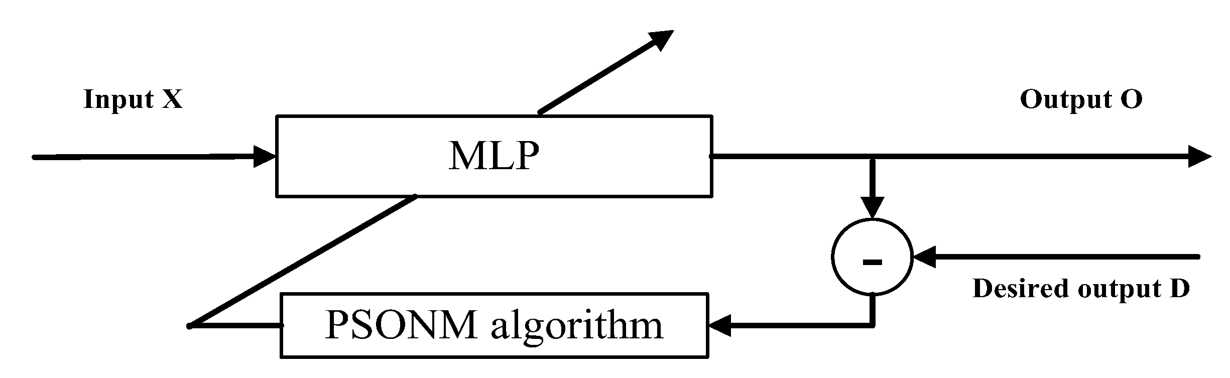
- The last contribution of PSONHM is to design a PSONHM-based trainer for MLPs. Classic learning methods, such as Back Propagation (BP), may lead MLPs to local minima rather than the global minimum. Neighborhood method, crossover operator and historical memory can enhance the exploitation and exploration capability of PSONHM. Then, it can help PSONHM find the optimal choice of weights and biases in the ANN and achieve the optimal result.
2. Related Work
2.1. PSO Framework
2.2. Improved PSO Based on Neighborhood
3. Proposed Modified Optimization Algorithm PSONHM
3.1. Motivations
3.2. Neighborhood Exploration Strategy
3.3. Property of Stagnation
3.4. Inertia Weight Assignments Based on Historical Memory
| Algorithm 1. PSONHM Algorithm. |
| 1: Initialize D(number of dimensions), NP, H, k, T, c0, c1 and c2 2: Initialize population randomly 3: Initialize position xi, velocity vi, personal best position pbesti, competitor of pbesti and global best position gbest of the NP particles (i = 1, 2, …, NP) 4: Initialize Mw,q according to Equation (8) 5: Index counter q = 1 6: while the termination criteria are not met do 7: Sw = ϕ 8: for i = 1 to NP do 9: r = Select from [1, k] randomly 10: w = Mw,r 11: if ti > = T 12: Compute velocity vi with neighborhood strategy according to Equation (4) 13: Update velocity vi by crossover operation according to Equations (5) and (6) 14: else 15: Compute velocity vi according to Equation (1) 16: end if 17: Update position xi according to Equation (2) 18: Calculate objective function value f(xi) 19: Calculate ti for next generation according to Equation (7) 20: end for 21: Update pbesti, gbest, and the competitor of pbesti (i = 1, 2, …, NP) 22: Update Mw,q based on Sw according to Equation (9) 23: q = q + 1 24: if q > k, q is set to 1 25: end while Output: the particle with the smallest objective function value in the population. |
4. Experiments and Discussion
4.1. General Experimental Setting
- unimodal problems f1–f3,
- simple multimodal problems f4–f16,
- hybrid problems f17–f22, and
- composite problems f23–f30.
4.2. Comparison with Nine Optimization Algorithms on 30 Dimensions
5. PSONHM for Training an MLP
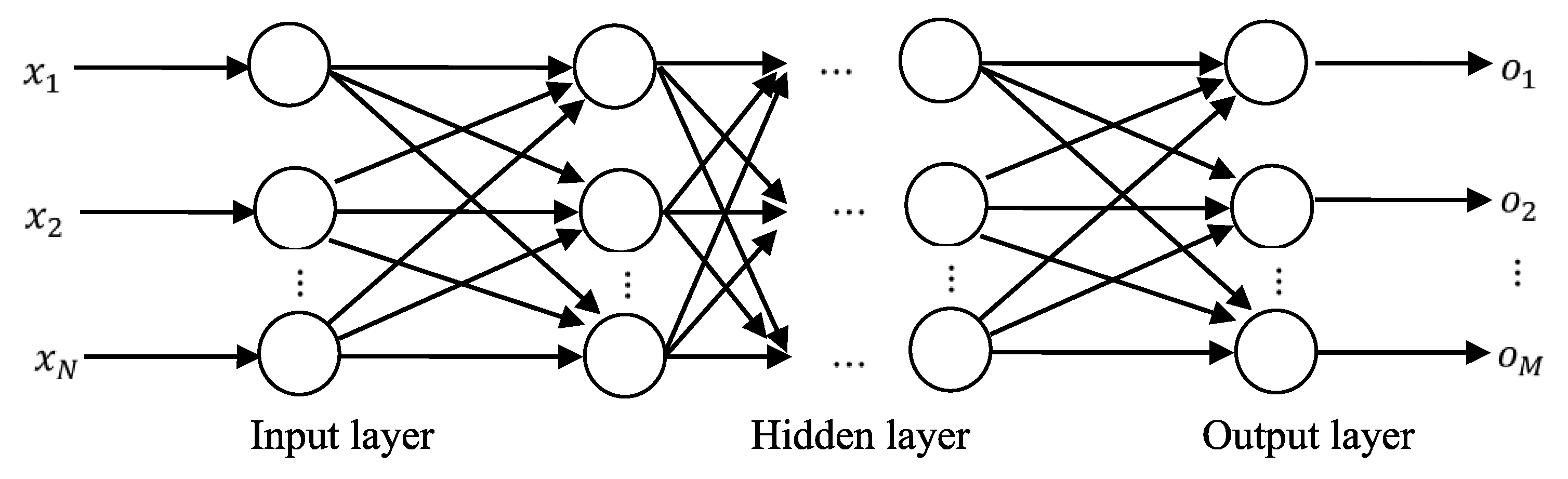
5.1. Multi-Layer Perceptron
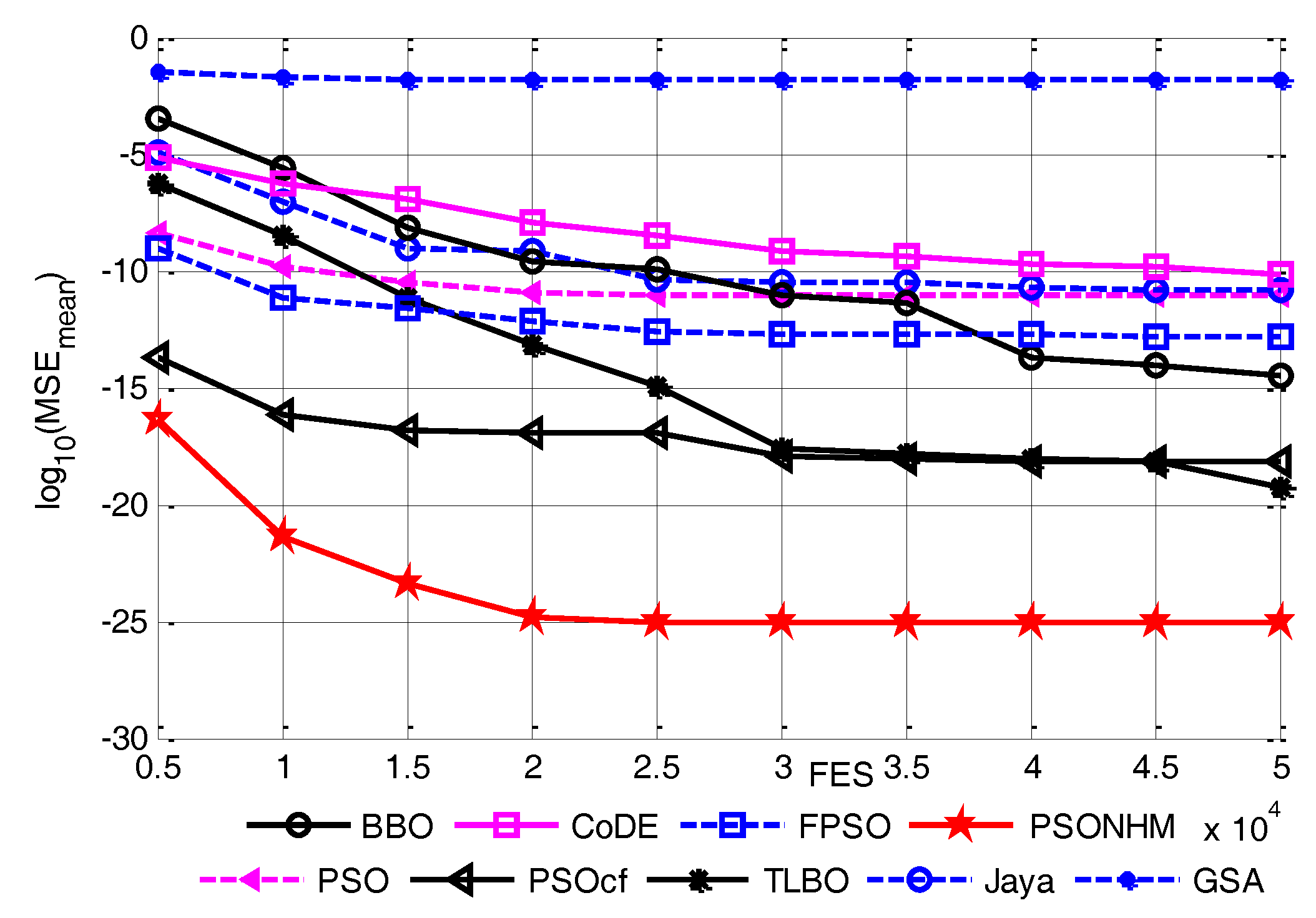
5.2. Classification Problems
5.2.1. Iris Flower Classification
5.2.2. Balloon Classification
6. Conclusions
Acknowledgments
Conflicts of Interest
References
- Mirjalili, S.; Mirjalili, S.M.; Lewis, A. Let A Biogeography-Based Optimizer Train Your Multi-Layer Perceptron. Inf. Sci. 2014, 268, 188–209. [Google Scholar] [CrossRef]
- Rosenblatt, F. The Perceptron, a Perceiving and Recognizing Automaton Project Para; Cornell Aeronautical Laboratory: Buffalo, NY, USA, 1957. [Google Scholar]
- Werbos, P. Beyond Regression: New Tools for Prediction and Analysis in the Behavioral Sciences. Ph.D. Thesis, Harvard University, Cambridge, MA, USA, 1974. [Google Scholar]
- Askarzadeh, A.; Rezazadeh, A. Artificial neural network training using a new efficient optimization algorithm. Appl. Soft Comput. 2013, 13, 1206–1213. [Google Scholar] [CrossRef]
- Gori, M.; Tesi, A. On the problem of local minima in backpropagation. IEEE Trans. Pattern Anal. Mach. Intell. 1992, 14, 76–86. [Google Scholar] [CrossRef]
- Mendes, R.; Cortez, P.; Rocha, M.; Neves, J. Particle swarms for feedforward neural network training. In Proceedings of the 2002 International Joint Conference on Neural Networks, Honolulu, HI, USA, 12–17 May 2002; pp. 1895–1899. [Google Scholar]
- Demertzis, K.; Iliadis, L. Adaptive Elitist Differential Evolution Extreme Learning Machines on Big Data: Intelligent Recognition of Invasive Species. Adv. Intell. Syst. Comput. 2017, 529, 1–13. [Google Scholar]
- Seiffert, U. Multiple layer perceptron training using genetic algorithms. In Proceedings of the European Symposium on Artificial Neural Networks, Bruges, Belgium, 25–27 April 2001; pp. 159–164. [Google Scholar]
- Blum, C.; Socha, K. Training feed-forward neural networks with ant colony optimization: An application to pattern classification. In Proceedings of the International Conference on Hybrid Intelligent System, Rio de Janeiro, Brazil, 6–9 December 2005; pp. 233–238. [Google Scholar]
- Tian, G.D.; Ren, Y.P.; Zhou, M.C. Dual-Objective Scheduling of Rescue Vehicles to Distinguish Forest Fires via Differential Evolution and Particle Swarm Optimization Combined Algorithm. IEEE Trans. Intell. Transp. Syst. 2016, 99, 1–13. [Google Scholar] [CrossRef]
- Guedria, N.B. Improved accelerated PSO algorithm for mechanical engineering optimization problems. Appl. Soft Comput. 2016, 40, 455–467. [Google Scholar] [CrossRef]
- Segura, C.; CoelloCoello, C.A.; Hernández-Díaz, A.G. Improving the vector generation strategy of Differential Evolution for large-scale optimization. Inf. Sci. 2015, 323, 106–129. [Google Scholar] [CrossRef]
- Liu, B.; Zhang, Q.F.; Fernandez, F.V.; Gielen, G.G.E. An Efficient Evolutionary Algorithm for Chance-Constrained Bi-Objective Stochastic Optimization. IEEE Trans. Evol. Comput. 2013, 17, 786–796. [Google Scholar] [CrossRef]
- Zaman, M.F.; Elsayed, S.M.; Ray, T.; Sarker, R.A. Evolutionary Algorithms for Dynamic Economic Dispatch Problems. IEEE Trans. Power Syst. 2016, 31, 1486–1495. [Google Scholar] [CrossRef]
- CarrenoJara, E. Multi-Objective Optimization by Using Evolutionary Algorithms: The p-Optimality Criteria. IEEE Trans. Evol. Comput. 2014, 18, 167–179. [Google Scholar]
- Cheng, S.H.; Chen, S.M.; Jian, W.S. Fuzzy time series forecasting based on fuzzy logical relationships and similarity measures. Inf. Sci. 2016, 327, 272–287. [Google Scholar] [CrossRef]
- Das, S.; Abraham, A.; Konar, A. Automatic clustering using an improved differential evolution algorithm. IEEE Trans. Syst. Man Cybern. Part A 2008, 38, 218–236. [Google Scholar] [CrossRef]
- Hansen, N.; Kern, S. Evaluating the CMA evolution strategy on multimodal test functions. In Parallel Problem Solving from Nature (PPSN), Proceedings of the 8th International Conference, Birmingham, UK, 18–22 September 2004; Springer International Publishing: Basel, Switzerland, 2004; pp. 282–291. [Google Scholar]
- Kirkpatrick, S.; Gelatt, C.D., Jr.; Vecchi, M.P. Optimization by Simulated Annealing. Science 1983, 220, 671–680. [Google Scholar] [CrossRef] [PubMed]
- Černý, V. Thermo dynamical approach to the traveling salesman problem: An efficient simulation algorithm. J. Optim. Theory Appl. 1985, 45, 41–51. [Google Scholar] [CrossRef]
- Simon, D. Biogeography-based optimization. IEEE Trans. Evol. Comput. 2008, 12, 702–713. [Google Scholar] [CrossRef]
- Lam, A.Y.S.; Li, V.O.K. Chemical-Reaction-Inspired Metaheuristic for Optimization. IEEE Trans. Evol. Comput. 2010, 14, 381–399. [Google Scholar] [CrossRef]
- Shi, Y.H. Brain Storm Optimization Algorithm; Advances in Swarm Intelligence, Series Lecture Notes in Computer Science; Springer: Berlin/Heidelberg, Germany, 2011; Volume 6728, pp. 303–309. [Google Scholar]
- Kennedy, J.; Eberhart, K. Particle swarm optimization. In Proceedings of the IEEE International Conference on Neural Networks, Perth, Australia, 27 November–1 December 1995; pp. 1942–1948. [Google Scholar]
- Bergh, F.V.D. An Analysis of Particle Swarm Optimizers. Ph.D. Thesis, University of Pretoria, Pretoria, South Africa, 2002. [Google Scholar]
- Clerc, M.; Kennedy, J. The particle swarm-explosion, stability, and convergence in a multidimensional complex space. IEEE Trans. Evol. Comput. 2002, 6, 58–73. [Google Scholar] [CrossRef]
- Krzeszowski, T.; Wiktorowicz, K. Evaluation of selected fuzzy particle swarm optimization algorithms. In Proceedings of the Federated Conference on Computer Science and Information Systems (FedCSIS), Gdansk, Poland, 11–14 September 2016; pp. 571–575. [Google Scholar]
- Alfi, A.; Fateh, M.M. Intelligent identification and control using improved fuzzy particle swarm optimization. Expert Syst. Appl. 2011, 38, 12312–12317. [Google Scholar] [CrossRef]
- Kwolek, B.; Krzeszowski, T.; Gagalowicz, A.; Wojciechowski, K.; Josinski, H. Real-Time Multi-view Human Motion Tracking Using Particle Swarm Optimization with Resampling. In Articulated Motion and Deformable Objects; Lecture Notes in Computer Science; Springer: Berlin/Heidelberg, Germany, 2012; Volume 7378, pp. 92–101. [Google Scholar]
- Sharifi, A.; Harati, A.; Vahedian, A. Marker-based human pose tracking using adaptive annealed particle swarm optimization with search space partitioning. Image Vis. Comput. 2017, 62, 28–38. [Google Scholar] [CrossRef]
- Gandomi, A.H.; Yun, G.J.; Yang, X.S.; Talatahari, S. Chaos-enhanced accelerated particle swarm optimization. Commun. Nonlinear Sci. Numer. Simul. 2013, 18, 327–340. [Google Scholar] [CrossRef]
- Mendes, R.; Kennedy, J.; Neves, J. The fully informed particle swarm simpler, maybe better. IEEE Trans. Evol. Comput. 2004, 8, 204–210. [Google Scholar] [CrossRef]
- Liang, J.J.; Qin, A.K.; Suganthan, P.N.; Baskar, S. Comprehensive Learning Particle Swarm Optimizer for Global Optimization of Multimodal Functions. IEEE Trans. Evol. Comput. 2006, 10, 281–295. [Google Scholar] [CrossRef]
- Nobile, M.S.; Cazzaniga, P.; Besozzi, D.; Colombo, R. Fuzzy self-turning PSO: A settings-free algorithm for global optimization. Swarm Evol. Comput. 2017. [Google Scholar] [CrossRef]
- Shi, Y.H.; Eberhart, R. A modified particle swarm optimizer. In Proceedings of the IEEE World Congress on Computational Intelligence, Anchorage, AK, USA, 4–9 May 1998; pp. 69–73. [Google Scholar]
- Shi, Y.H.; Eberhart, R.C. Empirical study of particle swarm optimizaiton. In Proceedings of the IEEE Congress on Evolutionary Computation, Washington, DC, USA, 6–9 July 1999; pp. 1950–1955. [Google Scholar]
- Das, S.; Abraham, A.; Chakraborty, U.K.; Konar, A. Differential evolution using a neighborhood-based mutation operator. IEEE Trans. Evol. Comput. 2009, 13, 526–553. [Google Scholar] [CrossRef]
- Omran, M.G.; Engelbrecht, A.P.; Salman, A. Bare bones differential evolution. Eur. J. Oper. Res. 2009, 196, 128–139. [Google Scholar] [CrossRef]
- Suganthan, P.N. Particle swarm optimiser with neighbourhood operator. In Proceedings of the IEEE Congress on Evolutionary Computation, Washington, DC, USA, 6–9 July 1999; Volume 3, pp. 1958–1962. [Google Scholar]
- Nasir, M.; Das, S.; Maity, D.; Sengupta, S.; Halder, U. A dynamic neighborhood learning based particle swarm optimizer for global numerical optimization. Inf. Sci. 2012, 209, 16–36. [Google Scholar] [CrossRef]
- Ouyang, H.B.; Gao, L.Q.; Li, S.; Kong, X.Y. Improved global-best-guided particle swarm optimization with learning operation for global optimization problems. Appl. Soft Comput. 2017, 52, 987–1008. [Google Scholar] [CrossRef]
- Zhang, J.Q.; Sanderson, A.C. JADE: Adaptive Differential Evolution with Optional External Archive. IEEE Trans. Evol. Comput. 2009, 13, 945–957. [Google Scholar] [CrossRef]
- Tanabe, R.; Fukunaga, A. Success-history based parameter adaptation for differential evolution. In Proceedings of the IEEE Congress on Evolutionary Computation, Cancún, Mexico, 20–23 June 2013; pp. 71–78. [Google Scholar]
- Liang, J.J.; Qu, B.Y.; Suganthan, P.N. Problem Definitions and Evaluation Criteria for the CEC 2014 Special Session and Competition on Single Objective Real-Parameter Numerical Optimization; Technical Report; Zhengzhou University and Nanyang Technological University: Singapore, 2013. [Google Scholar]
- Suganthan, P.N.; Hansen, N.; Liang, J.J.; Deb, K.; Chen, Y.P.; Auger, A.; Tiwari, S. Problem Definitions and Evaluation Criteria for the CEC2005 Special Session on Real-Parameter Optimization. 2005. Available online: http://www.ntu.edu.sg/home/EPNSugan (accessed on 9 January 2017).
- Wang, Y.; Cai, Z.X.; Zhang, Q.F. Differential evolution with composite trial vector generation strategies and control parameters. IEEE Trans. Evol. Comput. 2011, 15, 55–66. [Google Scholar] [CrossRef]
- Rao, R.V.; Savsani, V.J.; Vakharia, D.P. Teaching-learning-based optimization: A novel method for constrained mechanical design optimization problems. Comput. Aided Des. 2011, 43, 303–315. [Google Scholar] [CrossRef]
- Rao, R.V. Jaya: A simple and new optimization algorithm for solving constrained and unconstrained optimization problems. Int. J. Ind. Eng. Comput. 2016, 7, 19–34. [Google Scholar]
- Rashedi, E.; Nezamabadi, S.; Saryazdi, S. GSA: A gravitational search algorithm. Inf. Sci. 2009, 179, 2232–2248. [Google Scholar] [CrossRef]
- Shi, Y.H.; Eberhart, R.C. Fuzzy adaptive particle swarm optimization. In Proceedings of the Congress on Evolutionary Computation, Seoul, Korea, 27–30 May 2001; Volume 1, pp. 101–106. [Google Scholar]
- Bache, K.; Lichman, M. UCI Machine Learning Repository. 2013. Available online: http://archive.ics.uci.edu/ml (accessed on 9 January 2017).


| Algorithm | Parameter | Value |
|---|---|---|
| PSO | Population size (N) | 40 |
| Cognitive constant (C1) | 1.49445 | |
| Social Constant (C2) | 1.49445 | |
| Inertia constant (ω) | 0.9 to 0.4 | |
| Population size (N) | 100 | |
| PSOcf | Cognitive constant (C1) | 1.49445 |
| Social Constant (C2) | 1.49445 | |
| Inertia constant (ω) | 0.729 | |
| TLBO | Population size (N) | 100 |
| FPSO | Population size (N) | 80 |
| Cognitive constant (C1) | 2 | |
| Social Constant (C2) | 2 | |
| Jaya | Population size (N) | 100 |
| GSA | Population size (N) | 50 |
| Gravitational constant (G0) | 1 | |
| α | 20 | |
| BBO | Population size (N) | 50 |
| Mutation Probability | 0.08 | |
| Number of elites each generation | 8 | |
| CoDE | Population size (N) | 100 |
| Mutation factor (F) | [1.0 1.0 0.8] | |
| Crossover factor (CR) | [0.1 0.9 0.2] | |
| PSONHM | Population size (N) | 100 |
| Cognitive constant (C1) | 1.49445 | |
| Social Constant (C2) | 1.49445 | |
| Memory size | 5 | |
| p | 0.05 |
| F | PSO | PSOcf | TLBO | Jaya | GSA | BBO | CoDE | FPSO | PSONHM | |
|---|---|---|---|---|---|---|---|---|---|---|
| f1 | Fmean | 8.34 × 10⁶ | 6.44 × 10⁷ | 4.79 × 10⁵ | 7.05 × 10⁷ | 1.32 × 10⁷ | 1.89 × 10⁷ | 2.38 × 10⁴ | 1.14 × 10⁷ | 4.47 × 10⁵ |
| SD | 8.22 × 10⁶ | 7.75 × 10⁷ | 3.95 × 10⁵ | 2.00 × 10⁷ | 1.78 × 10⁶ | 1.33 × 10⁷ | 1.85 × 10⁴ | 1.14 × 10⁷ | 2.90 × 10⁵ | |
| Max | 2.77 × 10⁷ | 3.02 × 10⁸ | 1.58 × 10⁶ | 1.05 × 10⁸ | 1.79 × 10⁷ | 5.44 × 10⁷ | 8.61 × 10⁴ | 6.40 × 10⁷ | 9.92 × 10⁵ | |
| Min | 8.93 × 10⁴ | 3.89 × 10⁵ | 5.71 × 10⁴ | 3.58 × 10⁷ | 1.02 × 10⁷ | 1.71 × 10⁶ | 4840 | 1.97 × 10⁶ | 8.93 × 10⁴ | |
| Compare/rank | −/4 | −/8 | ≈/2 | −/9 | −/6 | −/7 | +/1 | −/5 | \/2 | |
| f2 | Fmean | 0.172 | 6.55 × 10⁹ | 22.2 | 7.05 × 10⁹ | 3.40 × 10⁹ | 4.26 × 10⁶ | 4.88 | 0.183 | 9.01 × 10⁻⁴ |
| SD | 0.529 | 5.33 × 10⁹ | 15.6 | 9.74 × 10⁸ | 1.86 × 10¹⁰ | 1.64 × 10⁶ | 2.10 | 0.664 | 1.35 × 10⁻³ | |
| Max | 2.56 | 1.95 × 10¹⁰ | 49.1 | 9.51 × 10⁹ | 1.02 × 10¹¹ | 1.01 × 10⁷ | 11.1 | 3.56 | 5.98 × 10⁻³ | |
| Min | 2.78 × 10⁻⁶ | 6.41 × 10⁻³ | 4.73 × 10⁻³ | 5.31 × 10⁹ | 2.16 × 10³ | 1.59 × 10⁶ | 2.48 | 4.16 × 10⁶ | 5.70 × 10⁻⁸ | |
| Compare/rank | −/2 | −/8 | −/5 | −/9 | −/7 | −/6 | −/4 | −/3 | \/1 | |
| f3 | Fmean | 6.04 | 2.44 × 10³ | 568 | 7.20 × 10⁴ | 8.29 × 10⁴ | 1.03 × 10⁴ | 1.63 × 10⁻⁴ | 16.21 | 0.370 |
| SD | 10.1 | 3.97 × 10³ | 358 | 1.42 × 10⁴ | 1.52 × 10³ | 7.91 × 10³ | 9.08 × 10⁻⁵ | 21.79 | 0.329 | |
| Max | 38.7 | 1.42 × 10⁴ | 1720 | 1.03 × 10⁵ | 8.52 × 10⁴ | 3.01 × 10⁴ | 4.15 × 10⁻⁴ | 89.75 | 0.968 | |
| Min | 3.67 × 10⁻³ | 8.23 × 10⁻² | 39.8 | 4.78 × 10⁴ | 7.93 × 10⁴ | 1.66 × 10³ | 5.56 × 10⁻⁵ | 5.80 × 10⁻² | 7.75 × 10⁻³ | |
| Compare/rank | −/3 | −/4 | −/3 | −/6 | −/7 | −/5 | +/1 | −/4 | \/2 | |
| −/≈/+ | 3/0/0 | 3/0/0 | 2/1/0 | 3/0/0 | 3/0/0 | 3/0/0 | 1/0/2 | 3/0/0 | \ | |
| Avg-rank | 3.00 | 6.67 | 3.33 | 8.00 | 6.67 | 6.00 | 2.00 | 4.00 | 1.67 | |
| F | PSO | PSOcf | TLBO | Jaya | GSA | BBO | CoDE | FPSO | PSONHM | |
|---|---|---|---|---|---|---|---|---|---|---|
| f4 | fmean | 167 | 332 | 54.9 | 443 | 1800 | 119 | 19.5 | 157 | 107 |
| SD | 26.2 | 238 | 41.2 | 88.9 | 6040 | 30.1 | 22.3 | 60.7 | 31.6 | |
| Max | 238 | 920 | 137 | 744 | 2.53 × 10⁴ | 180 | 70.3 | 270 | 145 | |
| Min | 124 | 68.5 | 1.56 × 10⁻² | 330 | 166 | 72.3 | 1.46 | 9.01 | 31.8 | |
| Compare/rank | −/6 | −/7 | +/2 | −/8 | −/9 | ≈/3 | +/1 | −/5 | \/3 | |
| f5 | fmean | 20.7 | 20.2 | 20.9 | 20.9 | 20.9 | 20.1 | 20.6 | 20.8 | 20 |
| SD | 0.149 | 0.25 | 7.02 × 10⁻² | 4.75 × 10⁻² | 4.29 × 10⁻² | 4.17 × 10⁻² | 4.13 × 10⁻² | 6.40 × 10⁻² | 0.204 | |
| Max | 20.9 | 20.8 | 21 | 21 | 21 | 20.2 | 20.6 | 20.9 | 20.8 | |
| Min | 20.4 | 20 | 20.6 | 20.8 | 20.8 | 20.1 | 20.5 | 20.7 | 20 | |
| Compare/rank | −/5 | −/3 | −/8 | −/7 | −/9 | −/2 | −/4 | −/6 | \/1 | |
| f6 | fmean | 13.1 | 17.8 | 11.5 | 35.1 | 34.5 | 14 | 20.4 | 14.7 | 9.19 |
| SD | 2.78 | 4.52 | 2.62 | 1.80 | 4.90 | 1.78 | 2.88 | 3.64 | 20.1 | |
| Max | 20 | 28.1 | 16.1 | 38.1 | 41.2 | 17.2 | 25.4 | 22.7 | 11.4 | |
| Min | 7.78 | 8.58 | 5.77 | 30.6 | 22.5 | 10.5 | 9.50 | 7.53 | 3.63 | |
| Compare/rank | −/3 | −/6 | −/2 | −/9 | −/8 | −/4 | −/7 | −/5 | \/1 | |
| f7 | fmean | 1.48 × 10⁻² | 79.7 | 1.34 × 10⁻² | 21 | 159 | 1.03 | 6.77 × 10⁻⁵ | 1.06 × 10⁻² | 0 |
| SD | 1.36 × 10⁻² | 43.9 | 1.99 × 10⁻² | 4.81 | 261 | 1.93 × 10⁻² | 5.44 × 10⁻⁵ | 1.19 × 10⁻² | 0 | |
| Max | 6.64 × 10⁻² | 205 | 7.57 × 10⁻² | 31.8 | 1050 | 1.07 | 3.05 × 10⁻⁴ | 4.40 × 10⁻² | 0 | |
| Min | 0 | 24.3 | 0 | 13.7 | 11.6 | 0.981 | 1.22 × 10⁻⁵ | 0 | 0 | |
| Compare/rank | −/5 | −/8 | −/4 | −/7 | −/9 | −/6 | −/2 | −/3 | \/1 | |
| f8 | fmean | 29.4 | 75.5 | 58.5 | 224 | 179 | 0.609 | 18.5 | 38.2 | 15 |
| SD | 7.01 | 23.1 | 11.7 | 12.8 | 52.8 | 0.244 | 1.93 | 13.6 | 3.15 | |
| Max | 44.7 | 131 | 81.5 | 254 | 448 | 1.39 | 22.2 | 80.5 | 18.9 | |
| Min | 16.9 | 31 | 39.7 | 204 | 140 | 0.204 | 13.8 | 15.9 | 5.96 | |
| Compare/rank | −/4 | −/7 | −/6 | −/9 | −/8 | +/1 | −/3 | −/5 | \/2 | |
| f9 | fmean | 77.1 | 123 | 61.3 | 262 | 214 | 51.1 | 139 | 82.9 | 50.5 |
| SD | 14.4 | 36.1 | 14.9 | 13.9 | 65.9 | 10.3 | 9.41 | 23.4 | 7.97 | |
| Max | 101 | 216 | 96.5 | 291 | 445 | 70.3 | 154 | 139 | 59.6 | |
| Min | 46.7 | 59.6 | 38.8 | 223 | 166 | 32.8 | 112 | 41.7 | 32.8 | |
| Compare/rank | −/4 | −/6 | −/3 | −/9 | −/8 | ≈/1 | −/7 | −/5 | \/1 | |
| f10 | fmean | 886 | 2370 | 1200 | 5630 | 4050 | 3.43 | 762 | 1.05 × 10³ | 522 |
| SD | 328 | 679 | 526 | 379 | 287 | 1.24 | 129 | 382 | 146 | |
| Max | 1600 | 3650 | 2400 | 6220 | 4400 | 7.10 | 991 | 1.61 × 10³ | 708 | |
| Min | 265 | 1330 | 6.87 | 4800 | 3290 | 1.13 | 535 | 279 | 139 | |
| Compare/rank | −/4 | −/7 | −/6 | −/9 | −/8 | +/1 | −/3 | −/5 | \/2 | |
| f11 | fmean | 2890 | 3440 | 6490 | 6880 | 4390 | 1810 | 4800 | 3.30 × 10³ | 2250 |
| SD | 661 | 760 | 352 | 367 | 140 | 250 | 208 | 1.05 × 10³ | 304 | |
| Max | 4300 | 4850 | 7150 | 7480 | 4620 | 2420 | 5230 | 6.85 × 10³ | 2630 | |
| Min | 1440 | 1740 | 5510 | 5990 | 4050 | 1180 | 4290 | 1.89 × 10³ | 1370 | |
| Compare/rank | −/3 | −/5 | −/8 | −/9 | −/6 | +/1 | −/7 | −/4 | \/2 | |
| f12 | fmean | 0.59 | 0.253 | 2.46 | 2.41 | 2.82 | 0.214 | 1.02 | 0.8201 | 0.198 |
| SD | 0.268 | 9.85 × 10⁻² | 0.241 | 0.331 | 0.352 | 5.40 × 10⁻² | 0.110 | 0.633 | 4.75 × 10⁻² | |
| Max | 1.67 | 0.468 | 2.98 | 2.98 | 3.37 | 0.334 | 1.23 | 2.56 | 0.251 | |
| Min | 0.273 | 0.103 | 2.07 | 1.66 | 1.98 | 0.127 | 0.794 | 0.139 | 6.94 × 10⁻² | |
| Compare/rank | −/4 | ≈/1 | −/8 | −/7 | −/9 | ≈/1 | −/6 | −/5 | \/1 | |
| f13 | fmean | 0.395 | 1.53 | 0.418 | 1.59 | 8.81 | 0.513 | 0.464 | 0.4214 | 0.339 |
| SD | 0.103 | 1.09 | 9.97 × 10⁻² | 0.323 | 0.938 | 0.103 | 6.44 × 10⁻² | 0.105 | 8.47 × 10⁻² | |
| Max | 0.594 | 4.33 | 0.619 | 2.48 | 10.2 | 0.691 | 0.546 | 0.701 | 0.555 | |
| Min | 0.186 | 0.556 | 0.262 | 0.982 | 6.74 | 0.264 | 0.325 | 0.277 | 0.197 | |
| Compare/rank | −/2 | −/7 | −/3 | −/8 | −/9 | −/6 | −/5 | −/4 | \/1 | |
| f14 | fmean | 0.308 | 22.1 | 0.275 | 9.61 | 139 | 0.402 | 0.284 | 0.313 | 0.361 |
| SD | 0.124 | 16.5 | 5.30 × 10⁻² | 1.83 | 115 | 0.177 | 3.46 × 10⁻² | 0.127 | 0.181 | |
| Max | 0.842 | 77.1 | 0.391 | 13.1 | 403 | 0.982 | 0.363 | 0.820 | 0.714 | |
| Min | 0.189 | 0.89 | 0.151 | 4.96 | 15.7 | 0.23 | 0.201 | 0.180 | 0.199 | |
| Compare/rank | ≈/1 | −/8 | ≈/1 | −/7 | −/9 | −/6 | ≈/1 | ≈/1 | \/1 | |
| f15 | fmean | 7.43 | 4290 | 9.28 | 56.5 | 43.6 | 14.1 | 13.4 | 7.34 | 5.84 |
| SD | 2.43 | 1.04 × 10⁴ | 3.73 | 49.1 | 14.5 | 3.01 | 0.865 | 2.34 | 2.01 | |
| Max | 15.4 | 4.23 × 10⁴ | 17.2 | 278 | 94.5 | 21.6 | 15.1 | 10.81 | 10.9 | |
| Min | 4.16 | 3.64 | 3.14 | 34.2 | 26.3 | 10.2 | 11.9 | 2.62 | 2.95 | |
| Compare/rank | −/3 | −/9 | −/4 | −/8 | −/7 | −/6 | −/5 | −/2 | \/1 | |
| f16 | fmean | 10.9 | 11.1 | 11.8 | 12.9 | 13.7 | 9.72 | 11.6 | 11.67 | 10.7 |
| SD | 0.599 | 0.62 | 0.311 | 0.173 | 0.238 | 0.681 | 0.230 | 0.515 | 0.619 | |
| Max | 12 | 12.5 | 12.5 | 13.3 | 14.1 | 11.3 | 11.9 | 12.42 | 11.9 | |
| Min | 9.69 | 9.55 | 11.2 | 12.6 | 13.2 | 8.81 | 11.1 | 10.08 | 9.81 | |
| Compare/rank | −/3 | −/4 | −/7 | −/8 | −/9 | ≈/1 | −/5 | −/6 | \/1 | |
| −/≈/+ | 12/1/0 | 12/1/0 | 11/1/1 | 13/0/0 | 13/0/0 | 6/4/3 | 11/1/1 | 12/1/0 | \ | |
| Avg-rank | 3.62 | 6.00 | 4.77 | 8.08 | 8.31 | 3.00 | 4.31 | 4.31 | 1.38 | |
| F | PSO | PSOcf | TLBO | Jaya | GSA | BBO | CoDE | FPSO | PSONHM | |
|---|---|---|---|---|---|---|---|---|---|---|
| f17 | Fmean | 7.41 × 10⁵ | 1.17 × 10⁶ | 2.10 × 10⁵ | 4.41 × 10⁶ | 1.65 × 10⁶ | 1.64 × 10⁶ | 1.47 × 10³ | 7.88 × 10⁵ | 1.07 × 10⁵ |
| SD | 7.71 × 10⁵ | 1.46 × 10⁶ | 1.66 × 10⁵ | 1.62 × 10⁶ | 1.60 × 10⁵ | 1.02 × 10⁶ | 235 | 9.02 × 10⁵ | 8.24 × 10⁴ | |
| Max | 3.05 × 10⁶ | 5.69 × 10⁶ | 7.79 × 10⁵ | 8.20 × 10⁶ | 1.94 × 10⁶ | 5.10 × 10⁶ | 1.87 × 10³ | 4.51 × 10⁶ | 2.93 × 10⁵ | |
| Min | 1.92 × 10⁴ | 3.45 × 10⁴ | 4.36 × 10⁴ | 8.17 × 10⁵ | 1.26 × 10⁶ | 3.24 × 10⁵ | 831 | 7.62 × 10⁴ | 4010 | |
| Compare/rank | −/4 | −/6 | −/3 | −/9 | −/8 | −/7 | +/1 | −/5 | \/2 | |
| f18 | Fmean | 5.77 × 10³ | 5.09 × 10⁷ | 2480 | 2.66 × 10⁷ | 286 | 3010 | 49.1 | 2.81 × 10⁵ | 1310 |
| SD | 6.10 × 10³ | 1.39 × 10⁸ | 4530 | 4.32 × 10⁷ | 65 | 2570 | 6.05 | 1.42 × 10⁶ | 1020 | |
| Max | 2.75 × 10⁴ | 5.03 × 10⁸ | 2.25 × 10⁴ | 1.71 × 10⁸ | 556 | 1.13 × 10⁴ | 60.3 | 7.80 × 10⁶ | 3020 | |
| Min | 251 | 437 | 77.8 | 5.03 × 10⁶ | 230 | 289 | 36.2 | 248 | 136 | |
| Compare/rank | −/6 | −/9 | −/4 | −/8 | +/2 | −/5 | +/1 | −/7 | \/3 | |
| f19 | Fmean | 15.1 | 25.9 | 12 | 37.1 | 217 | 29.7 | 7.15 | 15.6 | 6.88 |
| SD | 20.4 | 28 | 11 | 23.8 | 138 | 33.1 | 0.689 | 21.3 | 0.922 | |
| Max | 76.9 | 140 | 69.4 | 120 | 753 | 115 | 8.43 | 87.9 | 7.99 | |
| Min | 4.52 | 8.53 | 4.78 | 23 | 43.3 | 6.97 | 5.86 | 4.38 | 4.82 | |
| Compare/rank | −/4 | −/6 | −/3 | −/8 | −/9 | −/7 | −/2 | −/5 | \/1 | |
| f20 | Fmean | 368 | 1740 | 814 | 1.05 × 10⁴ | 2.31 × 10⁵ | 8020 | 30.4 | 537 | 257 |
| SD | 229 | 1800 | 388 | 3.62 × 10³ | 4.48 × 10⁴ | 6190 | 4.04 | 311 | 57.9 | |
| Max | 1330 | 7440 | 2020 | 2.06 × 10⁴ | 3.21 × 10⁵ | 2.80 × 10⁴ | 39.2 | 1.46 × 10³ | 340 | |
| Min | 890 | 223 | 381 | 3.58 × 10³ | 1.30 × 10⁵ | 648 | 24.6 | 189 | 152 | |
| Compare/rank | −/3 | −/6 | −/5 | −/8 | −/9 | −/7 | +/1 | −/4 | \/2 | |
| f21 | Fmean | 6.60 × 10⁴ | 4.41 × 10⁵ | 6.78 × 10⁴ | 9.02 × 10⁵ | 9.77 × 10⁵ | 7.51 × 10⁵ | 772 | 1.44 × 10⁵ | 2.20 × 10⁴ |
| SD | 7.53 × 10⁴ | 5.04 × 10⁵ | 3.98 × 10⁴ | 3.83 × 10⁵ | 2.02 × 10⁵ | 6.24 × 10⁵ | 112 | 1.53 × 10⁵ | 1.08 × 10⁴ | |
| Max | 3.38 × 10⁵ | 1.91 × 10⁶ | 1.60 × 10⁵ | 1.54 × 10⁶ | 1.55 × 10⁶ | 2.50 × 10⁶ | 982 | 6.74 × 10⁵ | 4.13 × 10⁴ | |
| Min | 1720 | 1.12 × 10⁴ | 1.92 × 10⁴ | 3.95 × 10⁵ | 6.47 × 10⁵ | 3.05 × 10⁴ | 583 | 4.66 × 10³ | 6200 | |
| Compare/rank | −/3 | −/6 | −/4 | −/8 | −/9 | −/7 | +/1 | −/5 | \/2 | |
| f22 | Fmean | 310 | 600 | 239 | 628 | 922 | 478 | 271 | 347 | 232 |
| SD | 136 | 218 | 106 | 113 | 161 | 200 | 153 | 173 | 82.4 | |
| Max | 620 | 1060 | 415 | 822 | 1270 | 896 | 627 | 777 | 330 | |
| Min | 22.5 | 204 | 40.2 | 349 | 736 | 35.2 | 25.8 | 20.8 | 411 | |
| Compare/rank | −/4 | −/7 | ≈/1 | −/8 | −/9 | −/6 | −/3 | −/5 | \/1 | |
| −/≈/+ | 6/0/0 | 6/0/0 | 5/1/0 | 6/0/0 | 5/0/1 | 6/0/0 | 2/0/4 | 6/0/0 | \ | |
| Avg-rank | 4.00 | 6.67 | 3.33 | 8.17 | 7.67 | 6.50 | 1.50 | 5.17 | 1.83 | |
| F | PSO | PSOcf | TLBO | Jaya | GSA | BBO | CoDE | FPSO | PSONHM | |
|---|---|---|---|---|---|---|---|---|---|---|
| f23 | Fmean | 315 | 353 | 315 | 349 | 246 | 316 | 315 | 315 | 315 |
| SD | 0.214 | 22 | 1.71 | 6.11 | 13.7 | 0.854 | 7.14 × 10⁻⁷ | 0.203 | 0.195 | |
| Max | 316 | 416 | 315 | 364 | 269 | 318 | 315 | 316 | 316 | |
| Min | 315 | 325 | 315 | 338 | 220 | 315 | 315 | 315 | 315 | |
| Compare/rank | ≈/3 | −/9 | +/2 | −/8 | +/1 | −/7 | ≈/3 | −/6 | \/3 | |
| f24 | Fmean | 235 | 257 | 200 | 252 | 207 | 233 | 249 | 236 | 230 |
| SD | 8.15 | 25.8 | 1.55 × 10⁻³ | 12.5 | 0.327 | 4.61 | 16.8 | 6.41 | 5.60 | |
| Max | 250 | 331 | 200 | 266 | 208 | 246 | 297 | 247 | 243 | |
| Min | 224 | 226 | 200 | 212 | 207 | 228 | 225 | 223 | 224 | |
| Compare/rank | −/5 | −/9 | +/1 | −/8 | +/2 | −/4 | −/7 | −/6 | \/3 | |
| f25 | Fmean | 210 | 214 | 200 | 220 | 201 | 207 | 202 | 212 | 210 |
| SD | 3.02 | 9.42 | 0.621 | 4.91 | 4.30 × 10⁻² | 1.58 | 0.139 | 4.15 | 2.55 | |
| Max | 218 | 241 | 203 | 229 | 201 | 210 | 203 | 221 | 216 | |
| Min | 206 | 204 | 200 | 210 | 200 | 205 | 202 | 206 | 206 | |
| Compare/rank | −/6 | −/8 | +/1 | −/9 | +/2 | +/4 | +/3 | −/7 | \/5 | |
| f26 | Fmean | 128 | 115 | 107 | 101 | 171 | 100 | 100 | 103 | 100 |
| SD | 55.9 | 33.7 | 25.2 | 0.411 | 37.7 | 0.114 | 0.529 | 18.3 | 0.411 | |
| Max | 332 | 200 | 200 | 103 | 200 | 100 | 100 | 200 | 100 | |
| Min | 100 | 100 | 100 | 100 | 108 | 100 | 100 | 100 | 100 | |
| Compare/rank | −/8 | −/7 | −/6 | −/4 | −/9 | −/2 | −/3 | −/5 | \/1 | |
| f27 | Fmean | 636 | 798 | 512 | 1130 | 210 | 570 | 400 | 622 | 427 |
| SD | 148 | 236 | 138 | 87.4 | 1.31 | 124 | 2.24 | 159 | 38.8 | |
| Max | 932 | 1090 | 844 | 1210 | 213 | 722 | 401 | 853 | 523 | |
| Min | 401 | 432 | 401 | 722 | 206 | 405 | 400 | 401 | 401 | |
| Compare/rank | −/7 | −/8 | −/4 | −/9 | +/1 | −/5 | ≈/2 | −/6 | \/2 | |
| f28 | Fmean | 1234 | 1570 | 1080 | 1208 | 213 | 977 | 1035 | 1.42 × 10³ | 985 |
| SD | 378 | 324 | 175 | 205 | 3.11 | 160 | 126 | 448 | 42.9 | |
| Max | 2400 | 2330 | 1700 | 1960 | 221 | 1630 | 1225 | 2.46 × 10³ | 1040 | |
| Min | 906 | 1130 | 887 | 1050 | 208 | 803 | 890 | 918 | 897 | |
| Compare/rank | −/7 | −/9 | −/5 | −/6 | +/1 | ≈/2 | −/4 | −/8 | \/2 | |
| f29 | Fmean | 2.14 × 10⁶ | 6.22 × 10⁶ | 1.44 × 10⁶ | 2.12 × 10⁶ | 244 | 1830 | 564 | 1.29 × 10⁶ | 1140 |
| SD | 6.71 × 10⁶ | 5.50 × 10⁶ | 3.28 × 10⁶ | 3.56 × 10⁶ | 8.55 | 504 | 206 | 4.91 × 10⁶ | 136 | |
| Max | 2.56 × 10⁷ | 1.71 × 10⁷ | 9.16 × 10⁶ | 1.02 × 10⁷ | 258 | 2850 | 733 | 1.96 × 10⁷ | 1290 | |
| Min | 1010 | 5.15 × 10⁴ | 1130 | 6.24 × 10⁴ | 229 | 1150 | 261 | 779 | 828 | |
| Compare/rank | −/8 | −/9 | −/6 | −/7 | +/1 | −/4 | +/2 | −/5 | \/3 | |
| f30 | Fmean | 4660 | 9.51 × 10⁴ | 3870 | 1.72 × 10⁴ | 251 | 6170 | 1.11 × 10³ | 9.50 × 10³ | 3040 |
| SD | 2260 | 7.58 × 10⁴ | 2870 | 1.46 × 10⁴ | 7.86 | 2670 | 179 | 9.06 × 10³ | 836 | |
| Max | 1.06 × 10⁴ | 2.35 × 10⁵ | 1.37 × 10⁴ | 6.91 × 10⁴ | 266 | 1.17 × 10⁴ | 1.45 × 10³ | 4.42 × 10⁴ | 4090 | |
| Min | 966 | 1860 | 994 | 7420 | 235 | 2090 | 772 | 1.20 × 10³ | 1440 | |
| Compare/rank | −/5 | −/9 | ≈/3 | −/8 | +/1 | −/6 | +/2 | −/7 | \/3 | |
| −/≈/+ | 7/1/0 | 8/0/0 | 4/1/3 | 8/0/0 | 1/0/7 | 6/1/1 | 3/2/3 | 8/0/0 | \ | |
| Avg-rank | 6.13 | 8.50 | 3.50 | 7.38 | 2.25 | 4.25 | 3.25 | 6.25 | 2.75 | |
| D | PSO | PSOcf | TLBO | Jaya | GSA | BBO | CoDE | FPSO | PSONHM | |
|---|---|---|---|---|---|---|---|---|---|---|
| 30 | −/≈/+ | 28/2/0 | 29/1/0 | 22/4/4 | 30/0/0 | 22/0/8 | 21/4/5 | 17/3/10 | 29/1/0 | \ |
| Avg-rank | 4.30 | 6.87 | 4.00 | 7.90 | 6.40 | 4.33 | 3.23 | 4.97 | 1.87 | |
| Algorithm | MSEmean | MSEstd | MSEmax | MSEmin | Classification Rate (%) |
|---|---|---|---|---|---|
| PSO | 2.67 × 10⁻² | 1.92 × 10⁻³ | 2.26 × 10⁻² | 2.97 × 10⁻² | 84.80 |
| PSOcf | 5.32 × 10⁻² | 1.00 × 10⁻¹ | 1.60 × 10⁻² | 3.40 × 10⁻¹ | 86.20 |
| TLBO | 2.01 × 10⁻² | 5.07 × 10⁻³ | 1.45 × 10⁻² | 3.14 × 10⁻² | 90.80 |
| Jaya | 6.31 × 10⁻² | 1.36 × 10⁻² | 4.95 × 10⁻² | 9.21 × 10⁻² | 80.93 |
| GSA | 1.60 × 10⁻¹ | 2.45 × 10⁻² | 0.127 | 1.99 × 10⁻¹ | 0.00 |
| BBO | 3.26 × 10⁻² | 4.63 × 10⁻³ | 2.63 × 10⁻² | 3.90 × 10⁻² | 83.00 |
| CoDE | 4.41 × 10⁻² | 5.82 × 10⁻³ | 5.37 × 10⁻² | 3.48 × 10⁻² | 67.06 |
| FPSO | 5.75 × 10⁻² | 9.97 × 10⁻² | 3.41 × 10⁻¹ | 2.46 × 10⁻² | 84.73 |
| PSONHM | 1.49 × 10⁻² | 3.80 × 10⁻³ | 7.11 × 10⁻³ | 2.12 × 10⁻² | 93.40 |
| Algorithm | MSEmean | MSEstd | MSEmax | MSEmin | Classification Rate (%) |
|---|---|---|---|---|---|
| PSO | 8.34 × 10⁻¹² | 2.56 × 10⁻¹¹ | 5.67 × 10⁻²⁰ | 8.14 × 10⁻¹¹ | 100 |
| PSOcf | 7.07 × 10⁻¹⁹ | 1.03 × 10⁻¹⁸ | 2.94 × 10⁻²⁵ | 3.06 × 10⁻¹⁸ | 100 |
| TLBO | 5.02 × 10⁻²⁰ | 1.58 × 10⁻¹⁹ | 4.49 × 10⁻³¹ | 5.01 × 10⁻¹⁹ | 100 |
| Jaya | 1.43 × 10⁻¹¹ | 2.48 × 10⁻¹¹ | 3.10 × 10⁻¹⁵ | 8.11 × 10⁻¹¹ | 100 |
| GSA | 1.41 × 10⁻² | 3.20 × 10⁻² | 4.85 × 10⁻⁵ | 1.04 × 10⁻¹ | 49.50 |
| BBO | 2.99 × 10⁻¹⁵ | 6.51 × 10⁻¹⁵ | 1.02 × 10⁻²⁰ | 2.02 × 10⁻¹⁴ | 100 |
| CoDE | 6.98 × 10⁻¹¹ | 7.39 × 10⁻¹¹ | 2.35 × 10⁻¹⁰ | 7.84 × 10⁻¹⁴ | 100 |
| FPSO | 1.45 × 10⁻¹³ | 1.88 × 10⁻¹³ | 5.46 × 10⁻¹³ | 4.32 × 10⁻¹⁶ | 100 |
| PSONHM | 9.27 × 10⁻²⁶ | 1.72 × 10⁻²⁵ | 1.05 × 10⁻³³ | 4.47 × 10⁻²⁵ | 100 |
© 2018 by the author. Licensee MDPI, Basel, Switzerland. This article is an open access article distributed under the terms and conditions of the Creative Commons Attribution (CC BY) license (http://creativecommons.org/licenses/by/4.0/).
Share and Cite
Li, W. Improving Particle Swarm Optimization Based on Neighborhood and Historical Memory for Training Multi-Layer Perceptron. Information 2018, 9, 16. https://doi.org/10.3390/info9010016
Li W. Improving Particle Swarm Optimization Based on Neighborhood and Historical Memory for Training Multi-Layer Perceptron. Information. 2018; 9(1):16. https://doi.org/10.3390/info9010016
Chicago/Turabian StyleLi, Wei. 2018. "Improving Particle Swarm Optimization Based on Neighborhood and Historical Memory for Training Multi-Layer Perceptron" Information 9, no. 1: 16. https://doi.org/10.3390/info9010016
APA StyleLi, W. (2018). Improving Particle Swarm Optimization Based on Neighborhood and Historical Memory for Training Multi-Layer Perceptron. Information, 9(1), 16. https://doi.org/10.3390/info9010016