A New Anomaly Detection System for School Electricity Consumption Data †


Department of ICT and Natural Sciences, Norwegian University of Science & Technology, Larsgårdsvegen 2, 6009 Ålesund, Norway
*
Author to whom correspondence should be addressed.
†
This paper is an extended version of our paper published in the 2017 IEEE International Conference on Big Data Analysis (ICBDA), Beijing, China, 10–12 March 2017.
Information 2017, 8(4), 151; https://doi.org/10.3390/info8040151
Submission received: 29 September 2017
/
Revised: 8 November 2017
/
Accepted: 16 November 2017
/
Published: 20 November 2017
(This article belongs to the Special Issue Supporting Technologies and Enablers for Big Data)
Abstract
:Anomaly detection has been widely used in a variety of research and application domains, such as network intrusion detection, insurance/credit card fraud detection, health-care informatics, industrial damage detection, image processing and novel topic detection in text mining. In this paper, we focus on remote facilities management that identifies anomalous events in buildings by detecting anomalies in building electricity consumption data. We investigated five models within electricity consumption data from different schools to detect anomalies in the data. Furthermore, we proposed a hybrid model that combines polynomial regression and Gaussian distribution, which detects anomalies in the data with 0 false negative and an average precision higher than 91%. Based on the proposed model, we developed a data detection and visualization system for a facilities management company to detect and visualize anomalies in school electricity consumption data. The system is tested and evaluated by facilities managers. According to the evaluation, our system has improved the efficiency of facilities managers to identify anomalies in the data.
1. Introduction
In recent years, with the ever-growing shortage of natural resources, energy has been a major political, social and economic topic. It is now widely accepted that conserving energy and reducing energy consumption is of paramount importance. In the UK, building energy consumption has increased at a rate of 0.5% per annum, which is approximately 40% of total energy consumption [1]. However, buildings are widely reported to utilize energy inefficiently [2].
Although many techniques have been extensively investigated for building energy consumption modeling to design a low-energy building, buildings often exceed the energy savings promised by their design. Anomalous events, such as faults in lighting equipment, can account for 2–11% of the total energy consumption for commercial buildings [3]. To identify anomalous events in buildings in time, increased attention has been given to remote facilities management.
Anomaly detection in building electricity consumption data is one of the most important methods to identify anomalous events in buildings. In different application domains, each anomaly detection problem has distinct features such as the nature of data, availability of labeled data and type of anomalies to be detected. Most of the existing anomaly detection techniques solve a specific formulation of the problem [4]. Applying concepts from different disciplines such as statistics, machine learning, and information theory to a specific problem formulation is a challenge in anomaly detection.
Different data mining techniques have been investigated and applied to electricity consumption data. Catterson et al. [5] presented an online contextual anomaly detection method for monitoring anomalies in the sensor data, such as loading, temperature, and network configuration, of a given transformer. McArthur et al. [6] described a multi-agent system to detect anomalies for condition monitoring of electrical plant behaviors. Jakkula et al. [7] introduced and compared different anomaly detection algorithms for identifying anomalies in household electricity consumption datasets.
In this paper, we present an innovative method and build a system to detect and visualize anomalies in school electricity consumption data for a facilities management company. The company provides facilities management service for over 40 schools in Scotland. Data on electricity consumption of these schools is recorded by their half hourly metering system. Every week facilities managers look over spreadsheet graphs of the data to identify anomalous events in school facilities, particularly unusually high electricity consumption. Our system is used to reduce this tedious and time-consuming eyeballing of the data. Parts of the results of the model investigation and the system development contributed to anomaly detection of school electricity consumption data have appeared in [8]. However, our research in this paper significantly differs from the previous work in the following aspects:
- Investigated other two models which are not described in [8].
- Presented the design of the data detection and visualization system.
- Evaluated the anomaly detection models and the system.
The paper is organized as follows. Section 2 introduces the school electricity consumption data used in our research and the related anomaly detection and visualization techniques. The investigation of anomaly detection models is described in Section 3. Section 4 shows the anomaly detection and visualization system for the school electricity consumption data. We evaluate the anomaly detection models and the system in Section 5. Finally, we present conclusions and discussions, and suggestions for future research in Section 6.
2. Background
2.1. Anomaly Detection
Anomaly detection, also referred to as outlier detection, is the process of detecting patterns in a given data set that do not conform to an established normal behavior [9]. Typically, the anomalous items correspond to some significant information in many diverse research areas, such as biomedical imaging, hyperspectral remote sensing, cybersecurity and industrial applications. Jansson et al. [10] applied stochastic anomaly detection methods to analyze eye-tracking data of Parkinson patients. Veracini et al. [11] presented an anomaly detection strategy for hyperspectral imagery based on a fully unsupervised Gaussian mixture learning. Feng et al. [12] outlined an anomaly detection method for industrial control systems that combines the analysis of network package contents and their time-series structure. Kumar [13] applied parallel and distributed anomaly detection algorithms to detect sophisticated cyberattacks on large-scale networks.
According to the availability of labeled data, there are three types of anomaly detection techniques:
- Supervised techniques build models for both anomalous data and normal data. An unseen data instance is classified as normal or an anomaly by comparing which model it belongs to.
- Semi-supervised techniques only build a model for normal data. An unseen data instance is classified as normal if it fits the model sufficiently well. Otherwise, the data instance is classified as anomalies.
- Unsupervised techniques do not need any training dataset. These approaches are based on the assumption that anomalies are much rarer than normal data in a given data set.
The nonconforming patterns in data are commonly called anomalies or outliers. They are classified into the three following categories [4]:
- Point Anomalies: A point anomaly is a single independent data instance which does not conform to a well defined normal behavior in a data set.
- Contextual Anomalies: A contextual anomaly is a data instance that is considered as an anomaly in a specific context, but not otherwise.
- Collective Anomalies: A collective anomaly is a collection of related data instances that are anomalous with respect to an entire data set.
In our research, semi-supervised anomaly detection is used to detect anomalies in school electricity data. Based on the experience of facilities managers, point and collective anomalies are the targets of the detection.
2.2. Time Series Data of School Electricity Consumption
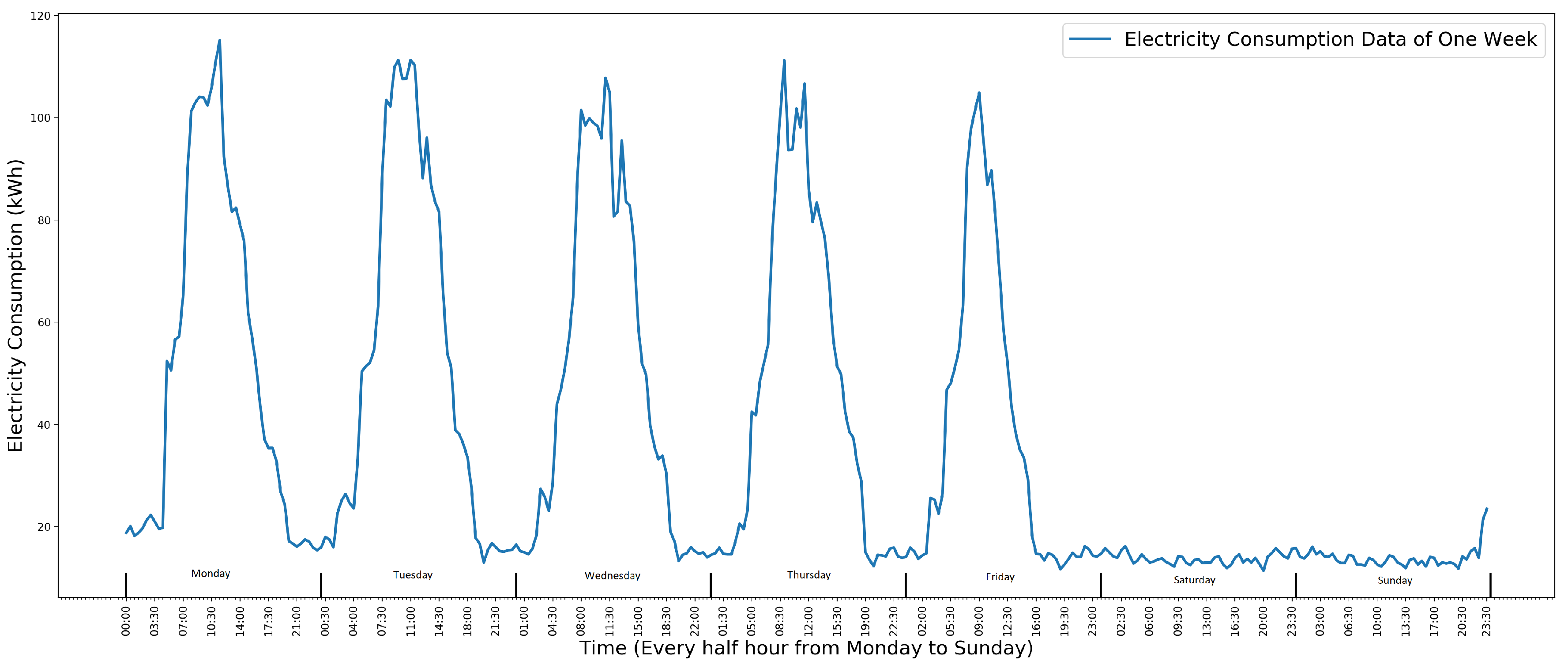
A time series is a sequence of data points that are ordered by a uniform time interval [14]. The school electricity consumption data used in this paper is in the form of a time series where the time interval is half an hour. It is recorded by a facilities management company. With half hourly frequency, the data for one week contains 336 data instances. Figure 1 shows one week’s electricity consumption data of a School from Monday to Sunday. In Figure 1, each data point represents the electricity consumption in the previous half hour. For weekly electricity consumption data, it fluctuates cyclically between Monday and Friday with a pattern and becomes steady with a small value.
With the school electricity consumption data, two types of anomalies are significant for facilities managers:
- One single high data point anomaly. It is often used to identify an anomalous meter because it is usually caused by a meter that records a wrong reading.
- A collection of continuous anomalies. It is used to identify anomalous electricity facilities, such as heating being on at the wrong time.
2.3. Data Visualization
Visualization plays an important role in exploring, analyzing, and understanding data. It has usually focused on developing techniques and systems to support the analysis of data, with limited analysis of the relationship between data and the construction of models on top of them [15]. However, instead of visualizing the result of data analysis, visualization is also important for improving the process of data modeling. Janetzko et al. [16] discussed and presented different possibilities for visualizing the power usage time series, which enables analysts to understand the power consumption behavior and to be aware of unexpected power consumption values.
In this research, the visualization enables researchers to communicate efficiently with domain experts who are mainly facilities managers. Since this research is to solve a practical anomaly detection problem in school electricity data, the expertise of domain experts is a significant basis. During the modeling process, each model is analyzed with visualization by researchers, which allows facilities managers to understand the analysis results and apply their domain expertise to improve the model. Furthermore, to understand school electricity consumption data before the analysis, the data is visualized in a cluster heat map. A cluster heat map is a graphical representation of data where the individual values contained in a matrix are represented as colors taken from a color scale [17]. To support the analysis of school electricity consumption data and refine the models, weekly data is visualized in a line chart in which detected anomalies are marked out. More details of visualizing the school electricity consumption data in a cluster heat map and a line chart are described in Section 4.2.
3. Anomaly Detection Models
To solve the practical anomaly detection problem in school electricity data, the expertise of domain experts is a significant basis for model selection and adjustment. The visualization of the model analysis enables domain experts who are mainly facilities managers to apply their expertise on model selection and adjustment. As a result, five models have been investigated with visualization for detecting anomalies in the school electricity data, including autoregressive, autoregressive-moving-average, polynomial regression, Gaussian kernel distribution and Gaussian distribution.
3.1. Autoregressive Model
Autoregressive (AR) model is widely used in time series analysis. AR is a linear regression model, but the output variable is regressed on its own previous values [18]. With an AR model, the future data instances in a time series can be predicted by the previous data.
An autoregressive is defined as:
where are parameters of model, c is a constant, and is a random error term with mean 0 and variance . p is the order of an AR model. An autoregressive model of order p is notated as . If the constant in an AR model is thought as a parameter, an model with a constant term can be thought as an model without the constant term.
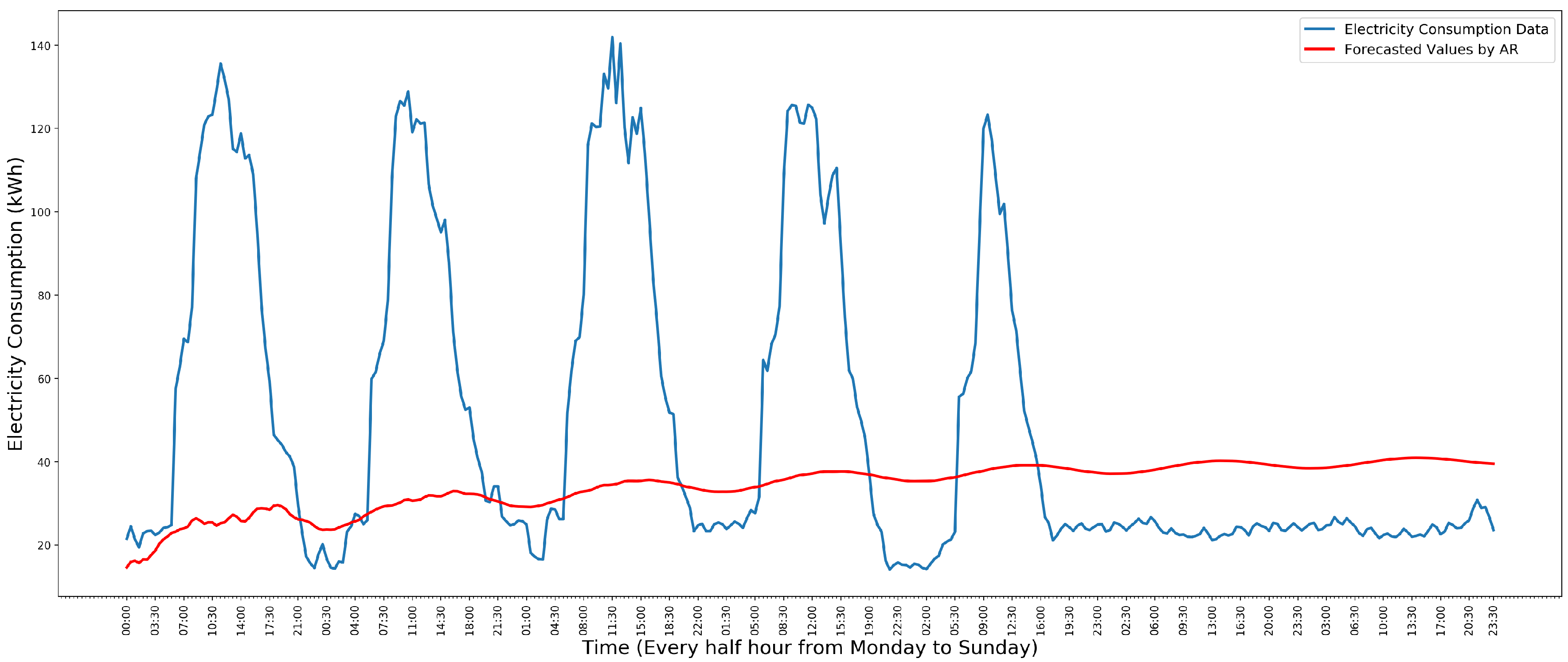
For predicting one week’s electricity consumption, this model is trained by its previous three weeks’ data. Several existing methods, such as Yule-Walker, Akaike/Bayesian Information Criterion, and Maximum Likelihood are adapted to estimate parameters for the models. This process is omitted in this paper. After training, we obtained an model. The model is investigated with one school’s electricity consumption data of the year 2011. Figure 2 shows the comparison of the 30th week’s electricity consumption data and the value predicted by .
In Figure 2, the blue line is the actual electricity consumption data. The red line is the predicted value. The results of other weeks’ data are similar to Figure 2. From Figure 2, it obviously shows that the predicted value cannot be used to detect anomalies in weekly electricity consumption data.
According to Figure 2, on weekdays, the data has the same trend that increases fast before 12:00 p.m. and then decreases fast after 12:00 p.m. AR model is a linear regression model. It captures either the trend before 12:00 p.m. or the trend after 12:00 p.m. When we fit an AR model with the data of the entire week, it is unable to capture the temporal structure of the data.
3.2. Autoregressive-Moving-Average Model
To improve the predicted accuracy, moving-average (MA) is added to the AR model. MA is a linear regression of the current value of a time series against current and previous random error terms, and is commonly used to smooth out short-term fluctuations and highlights long-term trends of a time series. A moving-average model is defined as:
where is mean of a series, are parameters of model, is a random error term with mean 0 and variance , q is the order of a MA model. An MA model of order q is notated as .
An autoregressive-moving-average (ARMA) model is a combination of AR and MA. Based on the definitions of AR and MA, an ARMA model is defined as:
where c is a constant, is a random error term with mean 0 and variance , and are parameters of model, p is the order of AR part, q is the order of MA part. An ARMA model with p autoregressive terms and q moving-average terms is notated as .
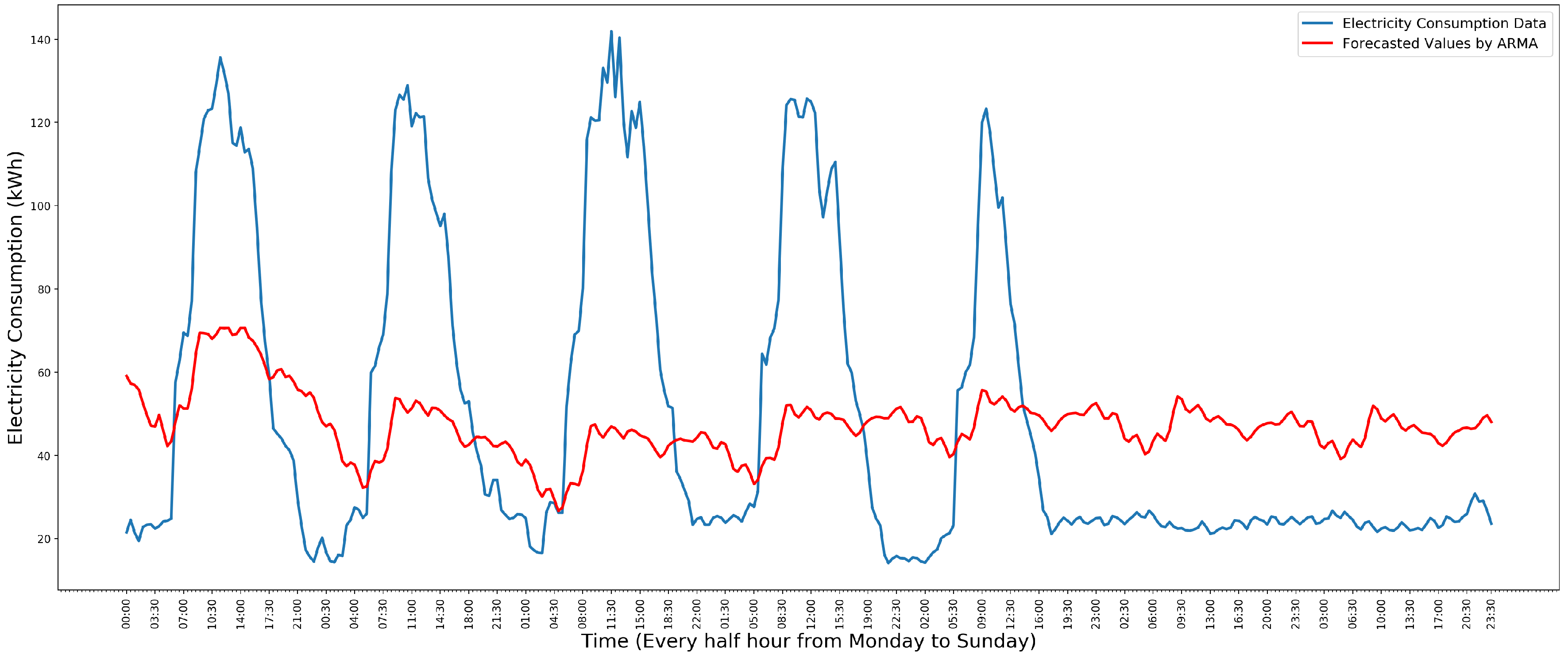
For predicting one week’s electricity consumption, an model is trained by its previous three week’s data. It is investigated with the same dataset used in the AR model section. Figure 3 shows the comparison of the 30th week’s electricity consumption data and the value predicted by .
With moving average, ARMA performs better than AR within school electricity consumption data. However, although the MA model smooths out the short-term fluctuation, the ARMA model still does not capture the entire temporal structure. This is because of a significant difference in the temporal structure of the data on weekdays and weekends.
3.3. Polynomial Regression Model
In order to avoid the volatility and capture the temporal structure of the school electricity consumption data, polynomial regression is investigated to model the variation of the data for each time slot through a year, since the data of a time slot in a week should fluctuate, slightly associated with the number of the week through one year.
Given a data set where is a scalar variable, the polynomial regression model is defined as:
where c is a constant, is a random error conditioned on , is the parameters of the model, and p is the order of the model.
The order of the polynomial regression model used in this paper is 11. Furthermore, to improve the numerical properties of the polynomial regression model, X is centered and scaled by:
where is the mean of X, and is the standard deviation of X.
This model is fitted to electricity consumption data of one time slot through a year. In one year, there are 52 data instances of each time slot. Figure 4 shows the polynomial regression model that is fitted to one school’s electricity consumption data for the first time slot of the year 2011.
In Figure 4, the blue stars are the electricity consumption data and the red line is the polynomial regression model that is fitted to the data.
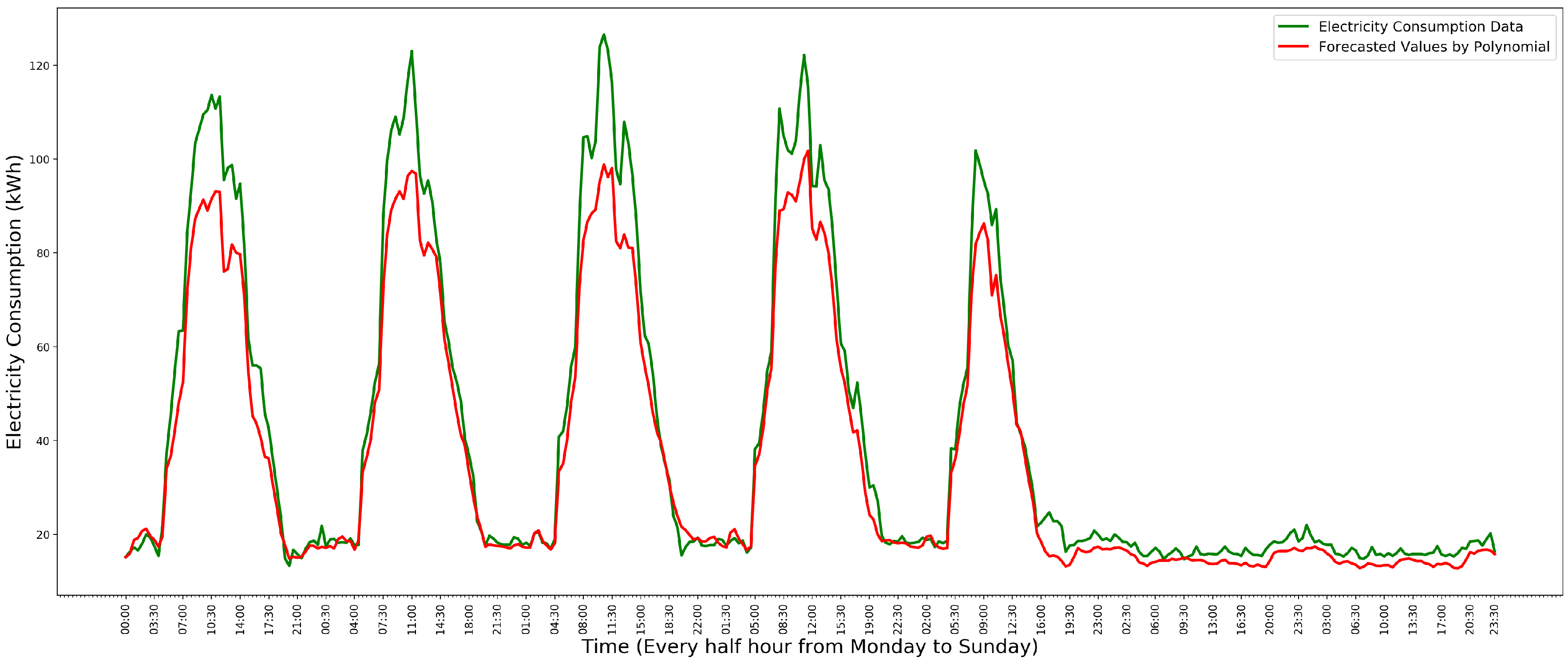
To predict one week’s electricity consumption data, each polynomial regression model is used to predict one data instance of one time slot. Figure 5 shows the predicted values of a week’s electricity consumption data, in which the green line is the data of the year 2011 and the red line is the predicted values.
In Figure 5, although the model does not predict the values of weekday sufficiently well, the predictions of Saturday and Sunday are accurate.
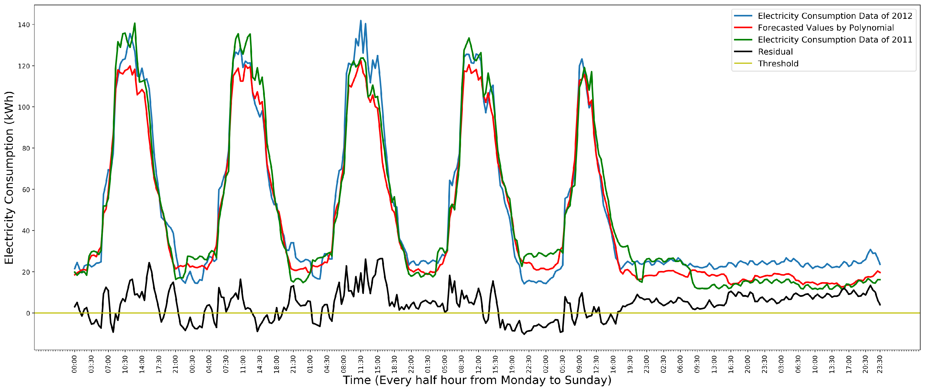
To detect anomalies in the data, the residual of each time slot is calculated. For one time slot, the residual is the difference between the actual value and the predicted value for this time slot. If the residual is greater than a threshold, the data instance will be detected as an anomaly. The threshold is computed for each school’s model, respectively, based on two labeled datasets. One is used to train the model. Then, the threshold is set and adjusted to guarantee that all the anomalies in Saturday and Sunday’s data can be detected in another dataset based on the model. Figure 6 shows the process of detecting anomalies in Saturday and Sunday’s data by the polynomial regression model.
In Figure 6, the green line is the data of the year 2011 that is used to train the model. The blue line is the data of the year 2012. The red line is the predicted values. The black line is the residual between the data of the year 2012 and the predicted values. The yellow line is , which is the threshold. Since the data of Saturday and Sunday in 2012 are much higher than that in 2011, the data of Saturday and Sunday in 2012 are anomalous. These anomalies can be detected by the residual. In Saturday and Sunday, if the residual of a data instance is greater than 0, the data instance will be detected as an anomaly. However, the residual of weekdays always fluctuates around 0. If we use the residual to detect the anomalies in a weekday, many normal data instances will be detected as anomalies. Therefore, this model cannot be used to detect the anomalies in a weekday.
3.4. Gaussian Kernel Distribution Model
An alternate approach to model the data in a week is to fit a distribution to the data instances from one time slot for a year. For each time slot, the data instance with a very low probability can be considered as an anomaly. Based on the features of the data, Gaussian kernel density estimation (KDE) is used to estimate the probability density function of the data.
Given a data set from an unknown continuous probability density function f, the Gaussian kernel density estimation is defined as:
where is the Gaussian kernel function, h is the bandwidth, and n is the number of the data instances in the data set.
In this research, the initial bandwidth h is estimated by minimizing the mean integrated squared error (MISE), the MISE is defined as:
and the initial bandwidth will be adjusted according to the model performance and facilities managers’ domain experience iteratively.
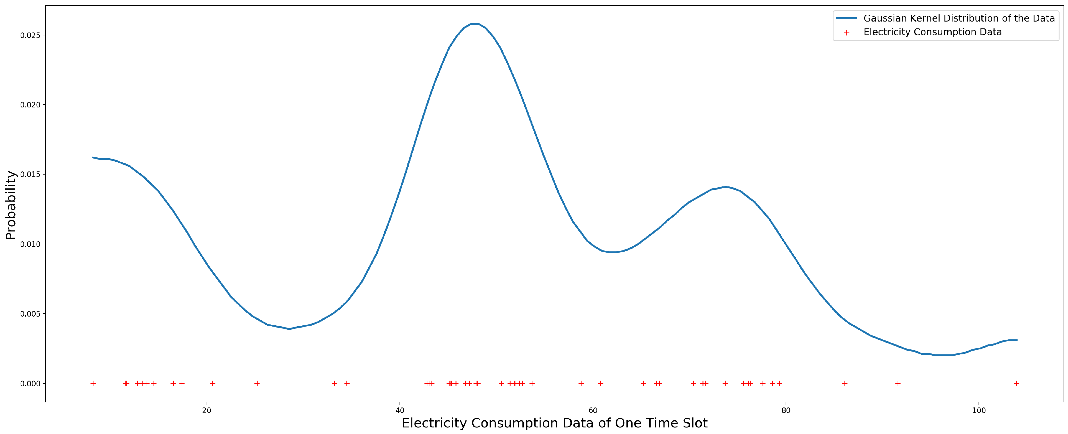
One school’s electricity consumption of the year 2011 is used to estimate the Gaussian kernel distribution for the data of each time slot. Figure 7 shows the Gaussian kernel distribution of the first time slot’s data, in which the red “+” is the electricity consumption data and the blue line is the Gaussian kernel distribution of the data.
To detect anomalies in weekly data, the probability of each data instance is calculated by the Gaussian kernel distribution of the corresponding time slot. If the probability of a data instance is less than a threshold of the time slot, the data instance will be considered as an anomaly. With the Gaussian kernel distribution of one time slot, the threshold for the time slot is given by:
where is the minimum probability of the Gaussian kernel distribution, is the maximum probability of the Gaussian kernel distribution, and is a coefficient. The process of adjusting the coefficient for different schools’ data is also based on two labeled datasets. One is used to train the model. Another is used to calculate the coefficient, which guarantees that all anomalies are detected in the dataset.
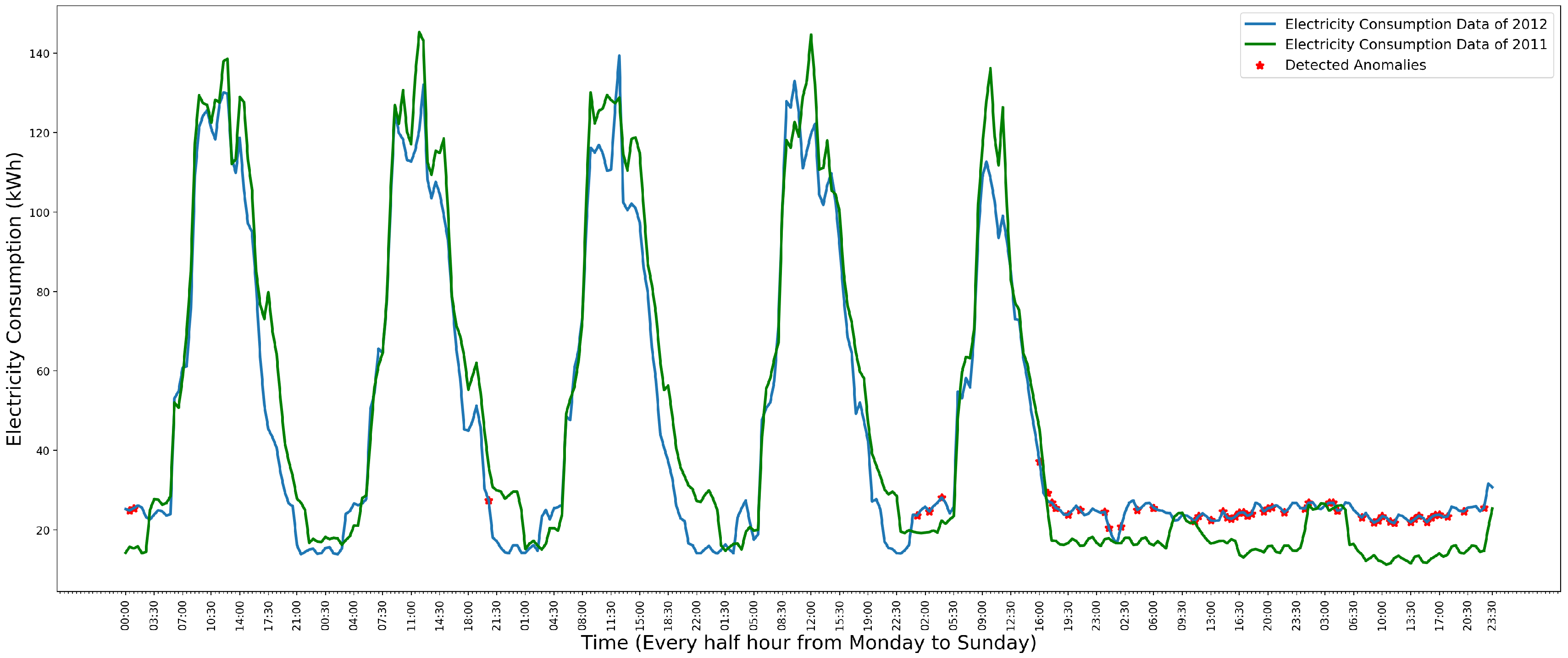
Figure 8 shows the detected anomalies in weekly data by the Gaussian kernel distribution model.
In Figure 8, the green line is the data of the year 2011, which is used to estimate the distribution. The blue line is the data of the year 2012. The red “*” is the detected anomalies in the data of the year 2012. Comparing the data of the year 2011 and 2012, the model has detected all the anomalies in the Monday, Friday, Saturday and Sunday’s data. However, the Gaussian kernel distribution model also comes with a low precision, which is shown in Figure 9.
In Figure 9, the green line is the data of the year 2011. The blue line is the data of the year 2012. The red “*” is the detected anomalies. Comparing the data of the year 2011 and 2012, the data of the year 2012 do not contain any anomalies. However, many normal data instances have been detected as anomalies. This is because some occasional activities such as a holiday on a weekday affect the electricity consumption, and this effect has been modeled by the Gaussian kernel distribution.
3.5. Gaussian Distribution Model
To avoid the low precision caused by the Gaussian kernel distribution, Gaussian distribution is adopted. With Gaussian distribution, for each time slot, if a data instance is greater than an upper bound, it will be considered as an anomaly. The probability density function of the Gaussian distribution is:
where is the mean of the data, and is the variance of the data.
Figure 10 shows the estimated Gaussian distribution of one school’s electricity consumption data for the first time slot of the year 2011. In Figure 10, the red “+” is the electricity consumption data. The blue line is the Gaussian distribution of the data.
To detect anomalies, the upper bound of one time slot is defined as:
where is the mean of the Gaussian distribution, is the standard deviation of the Gaussian distribution, and is a coefficient. The process of adjusting the coefficient is the same as previously described in Section 3.4.
Figure 11 shows the process of detecting anomalies in the data by the Gaussian distribution model.
In Figure 11, the green line is the data of 2011, which is used to fit the distribution. The blue line is the data of the year 2012. Comparing the data of the year 2011 and 2012, the model has detected the anomalies in Monday and Thursday of the year 2012. The thick part of the blue line is the detected anomalies. However, it does not detect the anomalies in Saturday and Sunday sufficiently well.
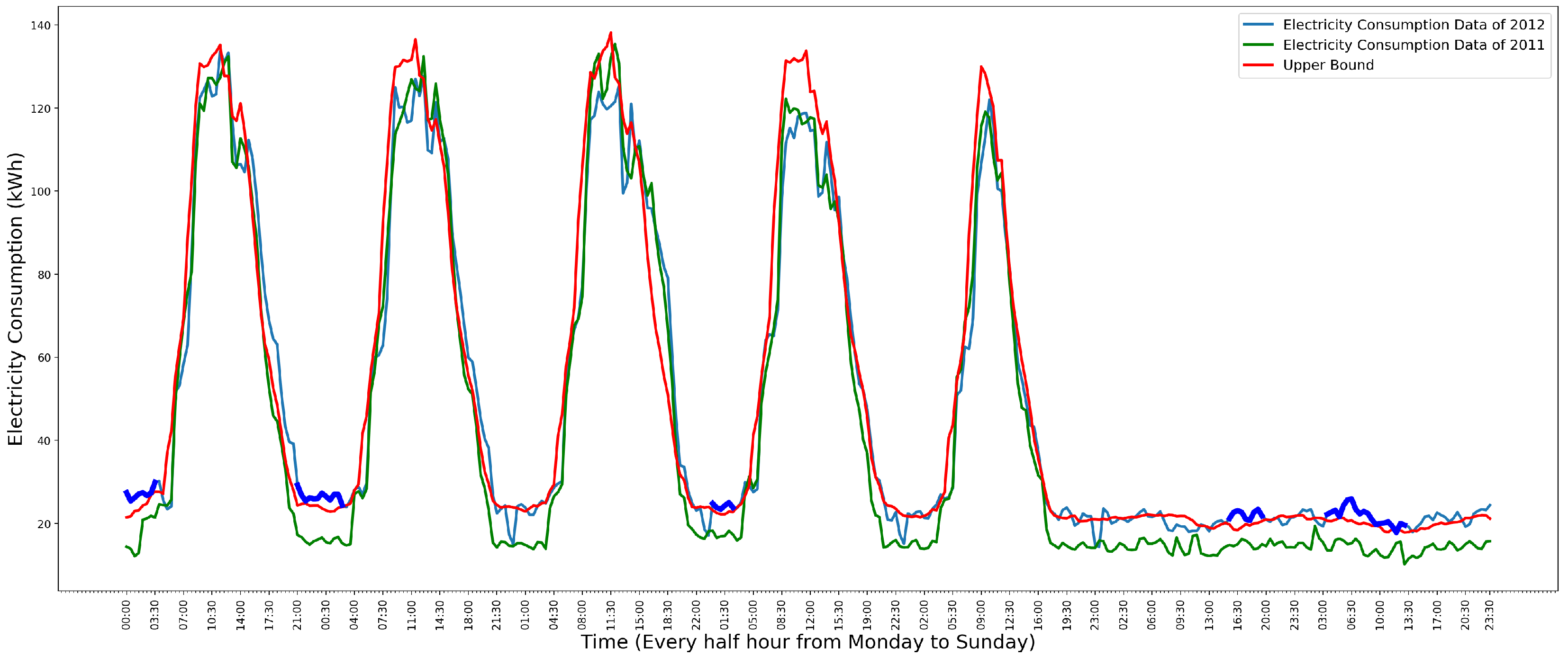
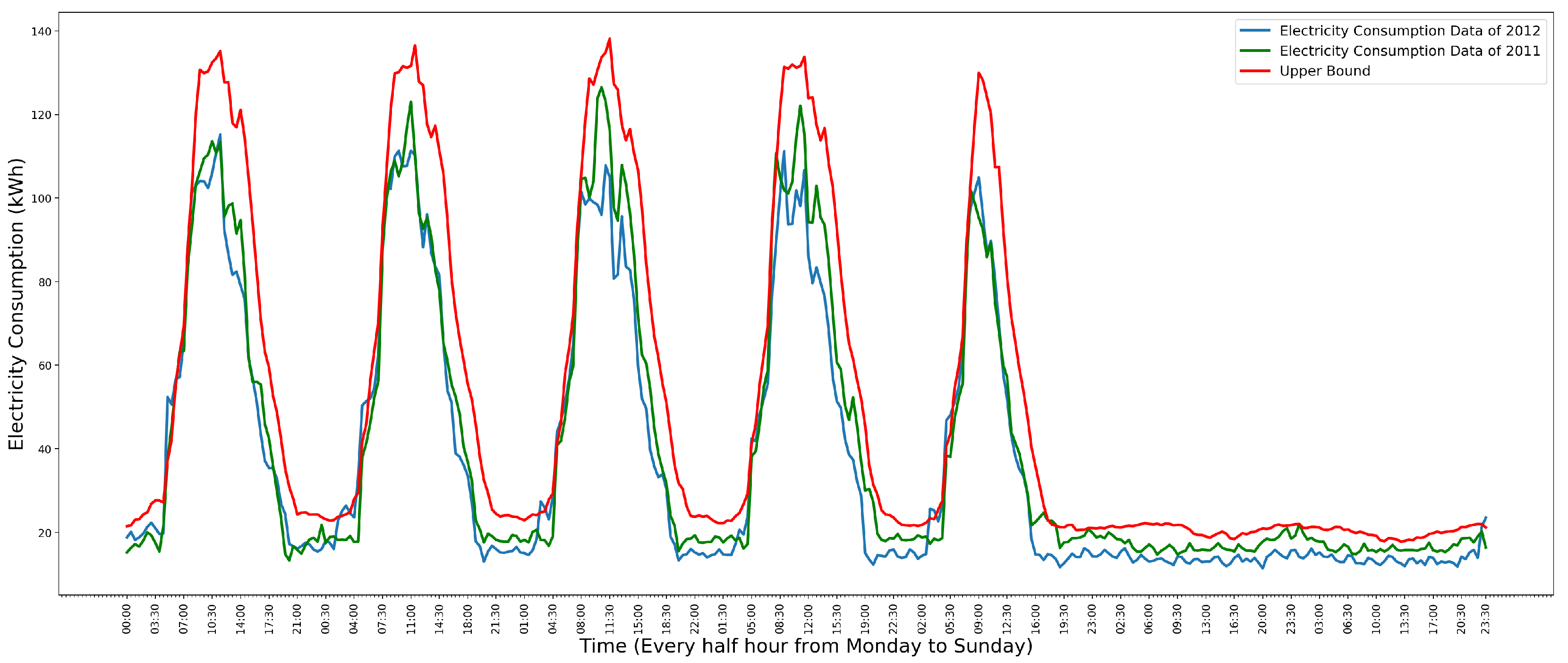
The Gaussian distribution model can avoid the low precision problem that appeared in the Gaussian Kernel distribution model. Effects caused by occasional activities are omitted by Gaussian distribution. Figure 12 shows the using Gaussian distribution model to detect anomalies in the weekly data which only contains normal data. In Figure 12, the green line is the data of the year 2011. The blue line is the data of the year 2012. The red line is the upper bound. It shows that all normal data of the year 2012 are less than the upper bound.
3.6. Model Selection
The polynomial regression model detects anomalies in the data of Saturday and Sunday. However, it is not suitable for the data of weekdays. The Gaussian kernel distribution model detects all anomalies in the data. However, it results in a high false positive and causes the low precision. The Gaussian distribution model detects anomalies in the data of weekdays with a low false positive. Therefore, in order to detect anomalies in weekly data with a low false negative and a high precision, a hybrid model that combines polynomial regression and Gaussian distribution is proposed:
where the coefficient and threshold c are adjusted according to different schools’ electricity consumption data as mentioned in Section 3.3 and Section 3.5.
4. Anomaly Detection and Visualization System
Based on the model proposed in the Section 3.6, we developed a data detection and visualization system for school electricity consumption data.
4.1. System Design
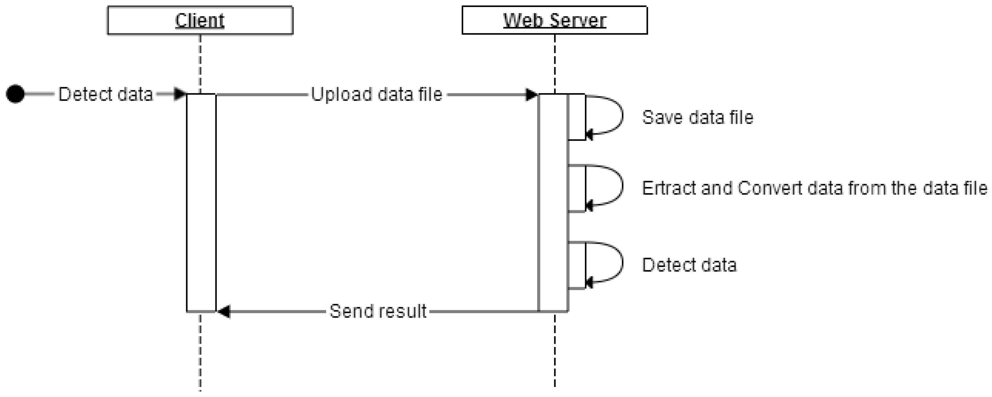
To simplify the user operation, client–server architecture is adapted to design and develop the data detection and visualization system. By using web browsers as clients in the system, there is no additional software need to be installed by users. Figure 13 shows the sequence diagram of data detection and visualization process of the system.
As shown in Figure 13, users only need to upload the data to the server. The data is automatically processed and detected on the server. The result of data detection is visualized in clients.
4.2. System Implementation
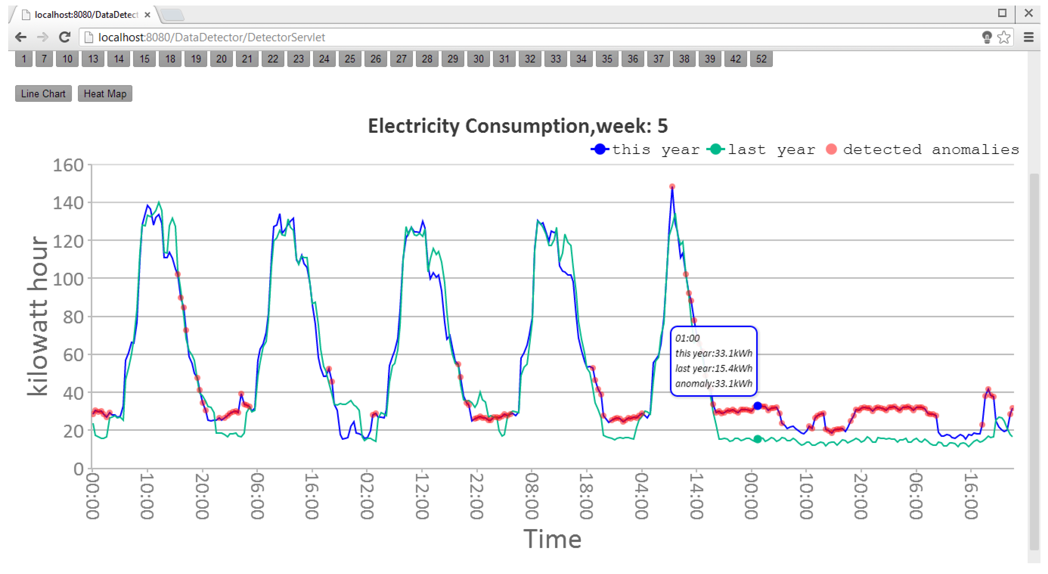
In the system, weekly data is visualized in a line chart and a cluster heat map, in which anomalies are marked out. Figure 14 shows the line chart of the 5th week’s electricity consumption data of a school.
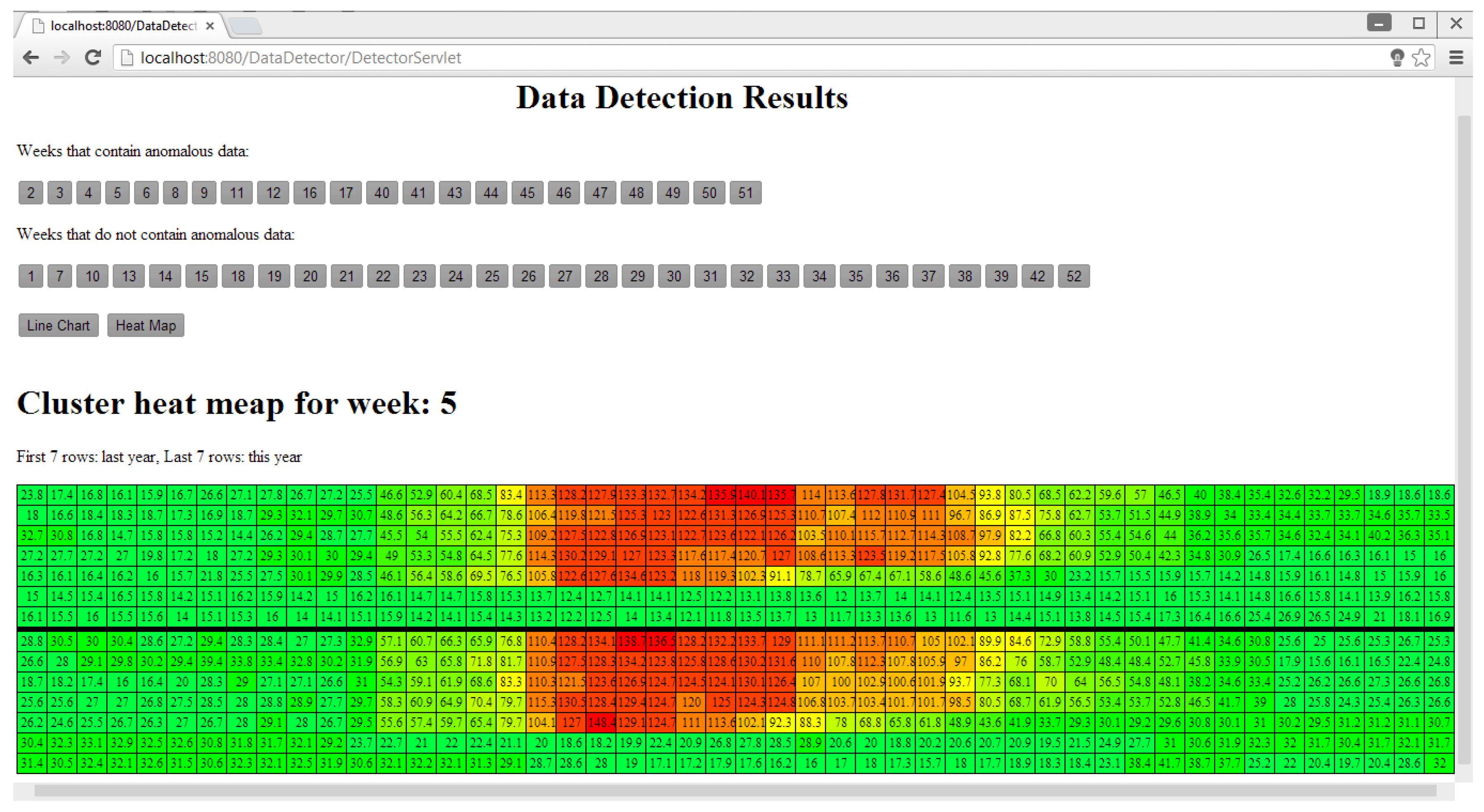
In Figure 14, the blue line is the data of the year 2012. The green line is the data of the year 2011, which is used to train the model. The red points are the detected single point anomaly and collective continuous anomalies in the data of the year 2012. Figure 15 shows the same data visualized in a cluster heat map.
In Figure 15, each row is daily electricity consumption data and the color of each cell is changed according to the data in which green represents low consumption, yellow represents medium consumption and red represents high consumption.
5. Evaluation
5.1. Model Evaluation
Recall, precision and false negative rate () are three common criteria used for evaluating anomaly detection methods, which are given as:
where (true positive) is the number of correctly detected anomalies, (false positive) is the number of normal instances that have been detected as anomalies, and (false negative) is the number of anomalies that have not been detected as anomalies.
For different schools’ electricity consumption data, the model proposed in Section 3.6 is trained to guarantee that all anomalies in the dataset are detected. This training criterion is requested by facilities managers based on their domain expertise. If a week with anomalies is not successfully detected, the whole system will be useless for facilities managers. Therefore, of the model is constant 0. This results in of the model being constant 0 and of the model being constant 1. Accordingly, is used as the only one criterion for the model evaluation. A low precision means that facilities managers need to check many incorrectly detected anomalies that actually are normal data instances.
The model is evaluated with three schools’ electricity consumption data, in which anomalies are labeled by facilities managers. Figure 16 shows the precision of anomaly detection result for three schools’ weekly data of the year 2012. The detailed tables of precision data are shown in the appendix.
In Figure 16, since of the model is 0, precision 0 means that there are no anomalies in those weeks’ data. Therefore, precision 0 is considered the same as the precision 100%. Precision 100% means that all anomalies have been correctly detected in the corresponding weeks’ data with zero FP. Precision between 0 and 100% means that all anomalies have been detected in the corresponding week’s data with non-zero FP. According to Figure 16, there are weeks of data have a 100% precision, weeks of data have a 0 precision, and weeks of data have an average precision that is higher than 70%. In total, the average precision of the model is higher than 91%.
5.2. System Evaluation
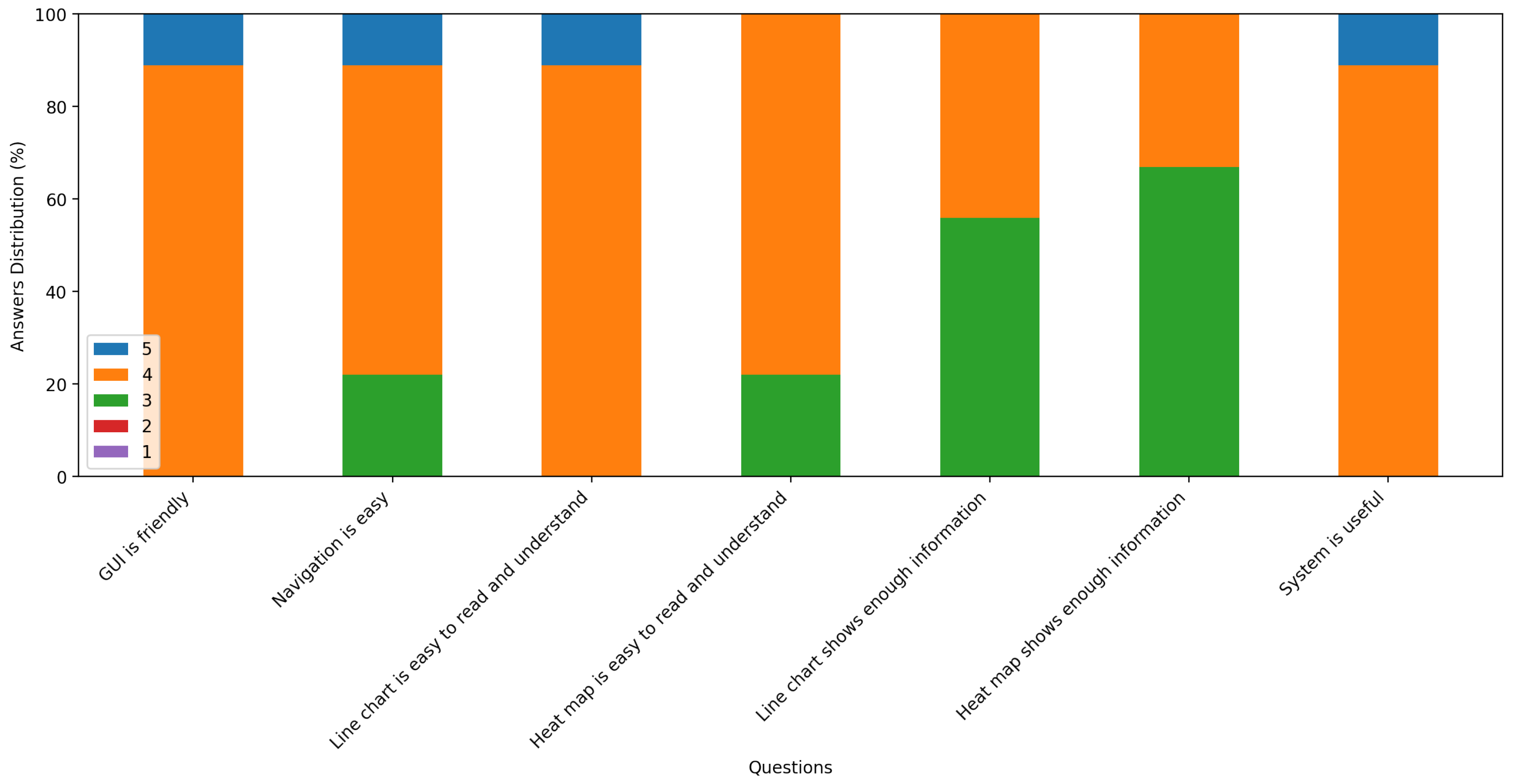
The system is evaluated by making a questionnaire that is shown in the appendix. There are nine facilities managers from a facilities management company participated in the evaluation. They used the system to detect different schools’ electricity consumption data and filled the questionnaire. For all questions, 5 represents the most positive answer and 1 the most negative answer. The statistical result of each question is shown in Figure 17. As the responses shown, facilities managers generally think:
- The system is easy to use.
- The visualization of anomaly detection is easy to read and understand.
- The system has improved their efficiency for identifying anomalies in school electricity consumption data.
6. Conclusions
In this paper, we have examined five models to detect anomalies in electricity consumption data. Moreover, we proposed a hybrid model that combines polynomial regression and Gaussian distribution. During the data modeling process, we integrated visualization techniques and data analysis. Based on the proposed model, we built a data detection and visualization system for a facilities management company, which has improved the efficiency of facilities managers to identify anomalies in the data. Furthermore, the variation of the proposed model can also be used for other types of time series that have similar characteristics.
Future research will focus on the automation of model fitting for different schools’ electricity consumption data. Currently, the model used in the system needs to be trained manually before detecting anomalies. Furthermore, since the model is trained by one year of data, long-term effects of the data have not been explored comprehensively. Therefore, optimizing the model with a larger dataset (e.g., data of 10 years), for example, investigating season and holiday effect on the model, is another research emphasis. Additionally, Visual Analytics (VA) [19] combine automatic data analytics with interactive data visualizations. It has been shown that visual analytics enable a virtuous cycle of user interaction, parameter refinement for algorithmic analysis methods so as to achieve rapid correction and improvement of human knowledge and decisions. We will further develop our anomaly detection methods in the VA framework for coupling interactive visual representations with underlying analytical processes.
Acknowledgments
The authors wish to thank the domain experts of the facilities management company for the valuable inputs and evaluation of the system described in this paper. The authors wish also to thank the valuable suggestions by the anonymous reviewers.
Author Contributions
Wenqiang Cui designed and performed the experiments; Wenqiang Cui and Hao Wang analyzed the data; Hao Wang contributed to the visualization analysis process; Wenqiang Cui and Hao Wang wrote the paper.
Conflicts of Interest
The authors declare no conflict of interest.
Appendix A. Questionnaire
Please mark your level in a red color of agreement to the following questions.
1: Strongly Disagree 2: Disagree 3: Neither 4: Agree 5: Strongly Agree
1. Do you think the graphical user interface is friendly?
1 2 3 4 5
2. Do you think navigating through different views is easy?
1 2 3 4 5
3. Do you think the line chart is easy to read and understand?
1 2 3 4 5
4. Do you think the heat map is easy to read and understand?
1 2 3 4 5
5. Do you think the line chart shows enough information?
1 2 3 4 5
6. Do you think the heat map shows enough information?
1 2 3 4 5
7. Do you think the system is useful?
1 2 3 4 5
8. Do you have any advice for the system?
Appendix B. Tables of Precision Data

Table A1.
The precision of anomaly detection results for the weekly data of School A.
| Week | 1 | 2 | 3 | 4 | 5 | 6 | 7 | 8 |
| Precision | 100% | 0 | 0 | 82.4% | 86.4% | 72.2% | 100% | 93.9% |
| Week | 9 | 10 | 11 | 12 | 13 | 14 | 15 | 16 |
| Precision | 0 | 100% | 68.7% | 71.4% | 100% | 100% | 100% | 0 |
| Week | 17 | 18 | 19 | 20 | 21 | 22 | 23 | 24 |
| Precision | 0 | 100% | 100% | 100% | 100% | 100% | 100% | 100% |
| Week | 25 | 26 | 27 | 28 | 29 | 30 | 31 | 32 |
| Precision | 100% | 100% | 100% | 100% | 100% | 100% | 100% | 100% |
| Week | 33 | 34 | 35 | 36 | 37 | 38 | 39 | 40 |
| Precision | 100% | 100% | 100% | 100% | 100% | 100% | 100% | 43.1% |
| Week | 41 | 42 | 43 | 44 | 45 | 46 | 47 | 48 |
| Precision | 0 | 100% | 45.3% | 85.1% | 89% | 92.3% | 84.6% | 70.2% |
| Week | 49 | 50 | 51 | 52 | ||||
| Precision | 66.7% | 72.7% | 78.6% | 100% |
Table A2.
The precision of anomaly detection results for the weekly data of School B.
| Week | 1 | 2 | 3 | 4 | 5 | 6 | 7 | 8 |
| Precision | 100% | 86.2% | 71.9% | 72.4% | 86.4% | 89% | 100% | 72.7% |
| Week | 9 | 10 | 11 | 12 | 13 | 14 | 15 | 16 |
| Precision | 76.5% | 77.6% | 61.2% | 81.4% | 0 | 100% | 100% | 0 |
| Week | 17 | 18 | 19 | 20 | 21 | 22 | 23 | 24 |
| Precision | 0 | 0 | 87.2% | 100% | 100% | 100% | 100% | 100% |
| Week | 25 | 26 | 27 | 28 | 29 | 30 | 31 | 32 |
| Precision | 100% | 100% | 100% | 100% | 100% | 94.3% | 100% | 100% |
| Week | 33 | 34 | 35 | 36 | 37 | 38 | 39 | 40 |
| Precision | 76.2% | 100% | 100% | 79.6% | 100% | 100% | 0 | 0 |
| Week | 41 | 42 | 43 | 44 | 45 | 46 | 47 | 48 |
| Precision | 0 | 100% | 77.6% | 100% | 100% | 100% | 100% | 65% |
| Week | 49 | 50 | 51 | 52 | ||||
| Precision | 48% | 72.7% | 15% | 100% |
Table A3.
The precision of anomaly detection results for weekly data of School C.
| Week | 1 | 2 | 3 | 4 | 5 | 6 | 7 | 8 |
| Precision | 100% | 100% | 0 | 79.6% | 68.1% | 0 | 100% | 74.3% |
| Week | 9 | 10 | 11 | 12 | 13 | 14 | 15 | 16 |
| Precision | 100% | 100% | 100% | 100% | 100% | 100% | 100% | 100% |
| Week | 17 | 18 | 19 | 20 | 21 | 22 | 23 | 24 |
| Precision | 81.5% | 71.4% | 100% | 100% | 100% | 100% | 100% | 100% |
| Week | 25 | 26 | 27 | 28 | 29 | 30 | 31 | 32 |
| Precision | 100% | 100% | 100% | 100% | 100% | 100% | 100% | 100% |
| Week | 33 | 34 | 35 | 36 | 37 | 38 | 39 | 40 |
| Precision | 100% | 100% | 100% | 100% | 0 | 100% | 100% | 100% |
| Week | 41 | 42 | 43 | 44 | 45 | 46 | 47 | 48 |
| Precision | 100% | 100% | 100% | 78.9% | 64.4% | 0 | 71.8% | 0 |
| Week | 49 | 50 | 51 | 52 | ||||
| Precision | 38.6% | 32.6% | 80.3% | 100% |
References
- Perez-Lombard, L.; Ortiz, J.; Pout, C. A review on buildings energy consumption information. Energy Build. 2008, 40, 394–398. [Google Scholar] [CrossRef]
- Ardehali, M.M.; Smith, T.F.; House, J.M.; Klaassen, C.J. 4641 Building Energy Use and Control Problems: An Assessment of Case Studies. ASHRAE Trans. 2003, 109, 111–121. [Google Scholar]
- Heo, Y.; Choudhary, R.; Augenbroe, G. Calibration of building energy models for retrofit analysis under uncertainty. Energy Build. 2012, 47, 550–560. [Google Scholar] [CrossRef]
- Chandola, V.; Banerjee, A.; Kumar, V. Anomaly detection: A survey. ACM Comput. Surv. (CSUR) 2009, 41, 15. [Google Scholar] [CrossRef]
- Catterson, V.M.; McArthur, S.D.; Moss, G. Online conditional anomaly detection in multivariate data for transformer monitoring. IEEE Trans. Power Deliv. 2010, 25, 2556–2564. [Google Scholar] [CrossRef] [Green Version]
- McArthur, S.D.; Booth, C.D.; McDonald, J.; McFadyen, I.T. An agent-based anomaly detection architecture for condition monitoring. IEEE Trans. Power Syst. 2005, 20, 1675–1682. [Google Scholar] [CrossRef]
- Jakkula, V.; Cook, D. Outlier detection in smart environment structured power datasets. In Proceedings of the 2010 Sixth International Conference on Intelligent Environments (IE), Kuala Lumpur, Malaysia, 19–21 July 2010; pp. 29–33. [Google Scholar]
- Cui, W.; Hao, W. Anomaly Detection and Visualization of School Electricity Consumption Data. In Proceedings of the 2017 IEEE International Conference on Big Data Analysis (ICBDA), Beijing, China, 10–12 March 2017. [Google Scholar]
- Abraham, B.; Chuang, A. Outlier detection and time series modeling. Technometrics 1989, 31, 241–248. [Google Scholar] [CrossRef]
- Jansson, D.; Rosén, O.; Medvedev, A. Parametric and nonparametric analysis of eye-tracking data by anomaly detection. IEEE Trans. Control Syst. Technol. 2015, 23, 1578–1586. [Google Scholar] [CrossRef]
- Veracini, T.; Matteoli, S.; Diani, M.; Corsini, G. Fully unsupervised learning of Gaussian mixtures for anomaly detection in hyperspectral imagery. In Proceedings of the Ninth International Conference on Intelligent Systems Design and Applications (ISDA’09), Pisa, Italy, 30 November–2 December 2009; pp. 596–601. [Google Scholar]
- Feng, C.; Li, T.; Chana, D. Multi-level anomaly detection in industrial control systems via package signatures and lstm networks. In Proceedings of the 2017 47th Annual IEEE/IFIP International Conference on Dependable Systems and Networks (DSN), Denver, CO, USA, 26–29 June 2017; pp. 261–272. [Google Scholar]
- Kumar, V. Parallel and distributed computing for cybersecurity. IEEE Distrib. Syst. Online 2005, 6. [Google Scholar] [CrossRef]
- Yaffee, R.A.; McGee, M. An Introduction to Time Series Analysis and Forecasting: With Applications of SAS® and SPSS®; Academic Press: New York, NY, USA, 2000. [Google Scholar]
- Krause, J.; Perer, A.; Bertini, E. INFUSE: Interactive feature selection for predictive modeling of high dimensional data. IEEE Trans. Vis. Comput. Graph. 2014, 20, 1614–1623. [Google Scholar] [CrossRef] [PubMed]
- Janetzko, H.; Stoffel, F.; Mittelstädt, S.; Keim, D.A. Anomaly detection for visual analytics of power consumption data. Comput. Graph. 2014, 38, 27–37. [Google Scholar] [CrossRef]
- Wilkinson, L.; Friendly, M. The history of the cluster heat map. Am. Stat. 2009, 63. [Google Scholar] [CrossRef]
- Chatfield, C. The Analysis of Time Series: An Introduction; CRC Press: Boca Raton, FL, USA, 2003. [Google Scholar]
- Keim, D.; Andrienko, G.; Fekete, J.D.; Gorg, C.; Kohlhammer, J.; Melançon, G. Visual analytics: Definition, process, and challenges. Lect. Notes Comput. Sci. 2008, 4950, 154–176. [Google Scholar]
Figure 1.
One week’s electricity consumption data of a school. The x-axis is the electricity consumption (kWh). The y-axis is the time. Adapted from [8].
Figure 1.
One week’s electricity consumption data of a school. The x-axis is the electricity consumption (kWh). The y-axis is the time. Adapted from [8].

Figure 2.
Comparison of the 30th week’s electricity consumption data and the predicted value. The y-axis is the electricity consumption data (kWh). The x-axis is the time. Adapted from [8].
Figure 2.
Comparison of the 30th week’s electricity consumption data and the predicted value. The y-axis is the electricity consumption data (kWh). The x-axis is the time. Adapted from [8].

Figure 3.
Comparison of one week’s electricity consumption data and the predicted value. Adapted from [8].
Figure 3.
Comparison of one week’s electricity consumption data and the predicted value. Adapted from [8].

Figure 4.
Polynomial regression model fitted to one school’s electricity consumption data for the first time slot through the year 2011. The x-axis is the week number from 1 to 52. The y-axis is the electricity consumption data (kWh). Adapted from [8].
Figure 4.
Polynomial regression model fitted to one school’s electricity consumption data for the first time slot through the year 2011. The x-axis is the week number from 1 to 52. The y-axis is the electricity consumption data (kWh). Adapted from [8].
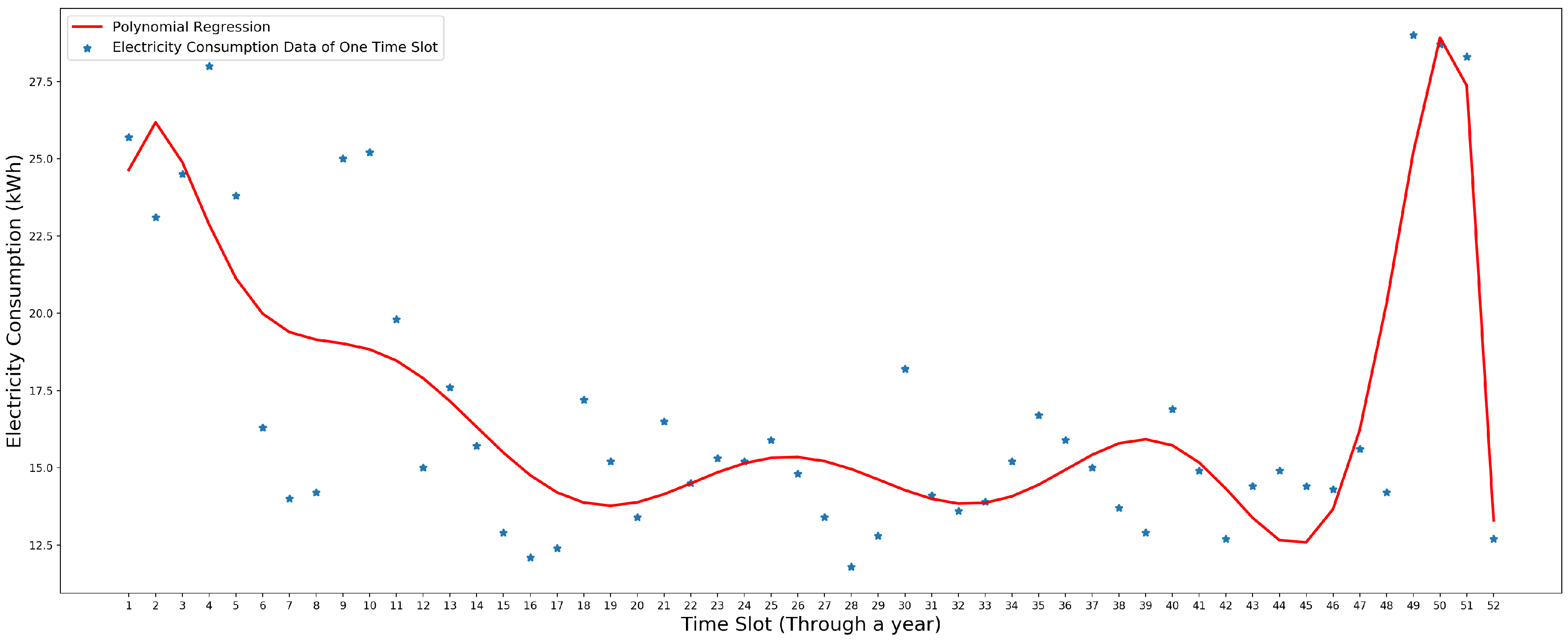
Figure 5.
Predicted values a week. Adapted from [8].
Figure 5.
Predicted values a week. Adapted from [8].

Figure 6.
Detecting anomalies in Saturday and Sunday. Adapted from [8].
Figure 6.
Detecting anomalies in Saturday and Sunday. Adapted from [8].

Figure 7.
Gaussian kernel distribution of the first time slot’s electricity consumption data. The x-axis is the electricity consumption data. The y-axis is the probability.
Figure 7.
Gaussian kernel distribution of the first time slot’s electricity consumption data. The x-axis is the electricity consumption data. The y-axis is the probability.

Figure 8.
Anomaly detection in weekly data by the Gaussian kernel distribution model. Adapted from [8].
Figure 8.
Anomaly detection in weekly data by the Gaussian kernel distribution model. Adapted from [8].

Figure 9.
Low precision of the Gaussian kernel distribution model. Adapted from [8].
Figure 9.
Low precision of the Gaussian kernel distribution model. Adapted from [8].
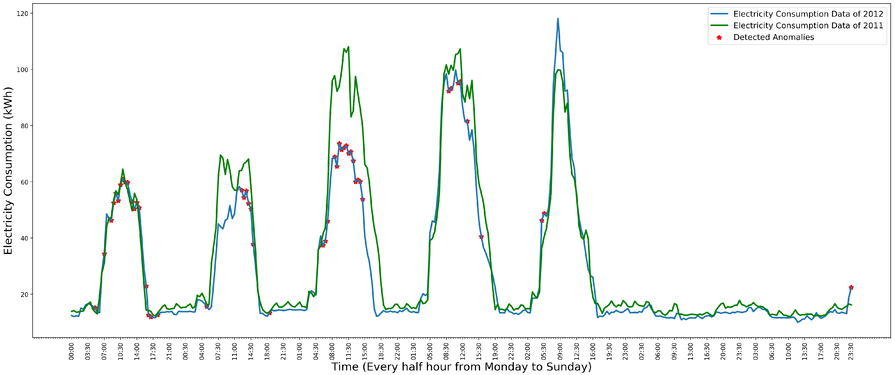
Figure 10.
Gaussian distribution of the first time slot’s electricity consumption data. Adapted from [8].
Figure 10.
Gaussian distribution of the first time slot’s electricity consumption data. Adapted from [8].
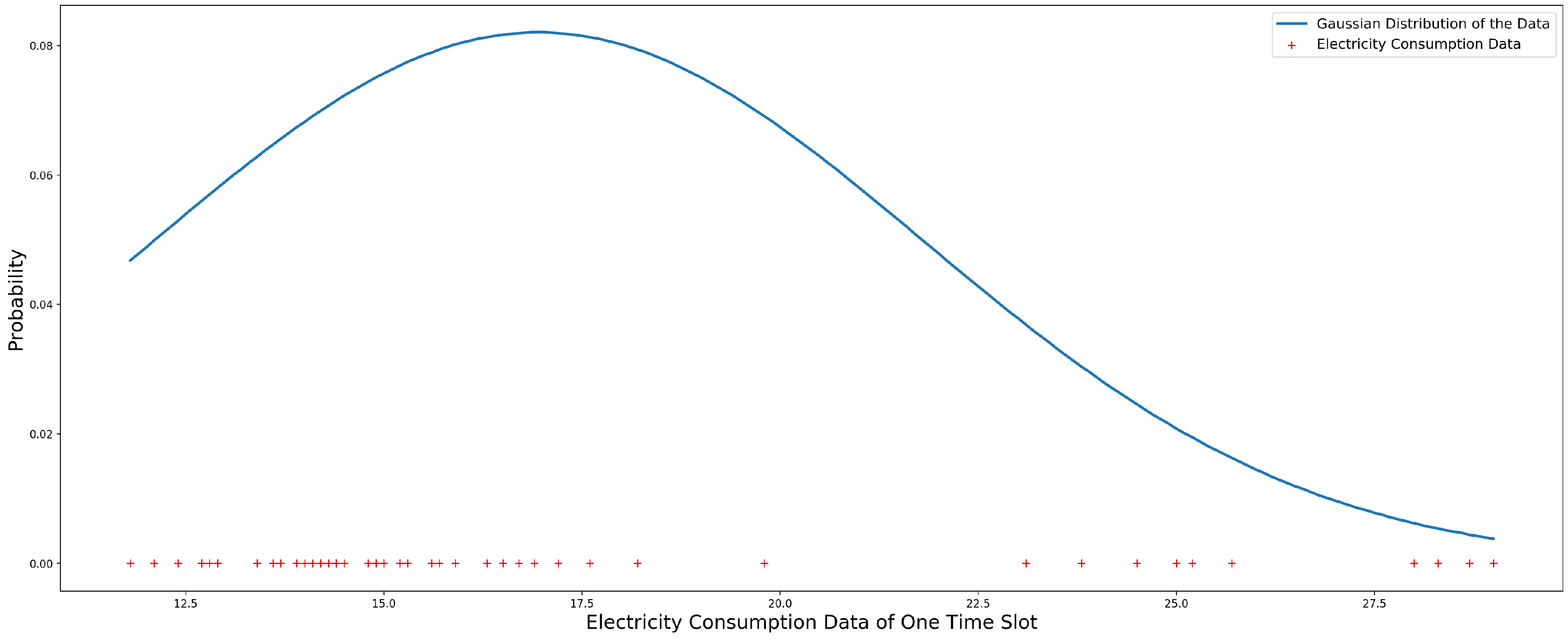
Figure 11.
Anomaly detection based on the Gaussian distribution model. The x-axis is the time. The y-axis is the electricity consumption data. Adapted from [8].
Figure 11.
Anomaly detection based on the Gaussian distribution model. The x-axis is the time. The y-axis is the electricity consumption data. Adapted from [8].

Figure 12.
Anomaly detection on normal weekly data based on Gaussian distribution model. Adapted from [8].
Figure 12.
Anomaly detection on normal weekly data based on Gaussian distribution model. Adapted from [8].

Figure 13.
Data detection process of the system.

Figure 14.
The line chart of the 5th week’s electricity consumption data of a school [8].
Figure 14.
The line chart of the 5th week’s electricity consumption data of a school [8].

Figure 15.
The heat map of the 5th week’s electricity consumption data of a school [8].
Figure 15.
The heat map of the 5th week’s electricity consumption data of a school [8].

Figure 16.
The precision of anomaly detection result for three schools’ weekly data of the year 2012.
Figure 16.
The precision of anomaly detection result for three schools’ weekly data of the year 2012.

Figure 17.
The statistical result of the questionnaire.
© 2017 by the authors. Licensee MDPI, Basel, Switzerland. This article is an open access article distributed under the terms and conditions of the Creative Commons Attribution (CC BY) license (http://creativecommons.org/licenses/by/4.0/).
Share and Cite
MDPI and ACS Style
Cui, W.; Wang, H. A New Anomaly Detection System for School Electricity Consumption Data. Information 2017, 8, 151. https://doi.org/10.3390/info8040151
AMA Style
Cui W, Wang H. A New Anomaly Detection System for School Electricity Consumption Data. Information. 2017; 8(4):151. https://doi.org/10.3390/info8040151
Chicago/Turabian StyleCui, Wenqiang, and Hao Wang. 2017. "A New Anomaly Detection System for School Electricity Consumption Data" Information 8, no. 4: 151. https://doi.org/10.3390/info8040151
Note that from the first issue of 2016, this journal uses article numbers instead of page numbers. See further details here.