Certain Competition Graphs Based on Intuitionistic Neutrosophic Environment


Department of Mathematics, University of the Punjab, New Campus, Lahore 54590, Pakistan
*
Author to whom correspondence should be addressed.
Information 2017, 8(4), 132; https://doi.org/10.3390/info8040132
Submission received: 7 September 2017
/
Revised: 18 October 2017
/
Accepted: 19 October 2017
/
Published: 24 October 2017
(This article belongs to the Special Issue Neutrosophic Information Theory and Applications)
Abstract
:The concept of intuitionistic neutrosophic sets provides an additional possibility to represent imprecise, uncertain, inconsistent and incomplete information, which exists in real situations. This research article first presents the notion of intuitionistic neutrosophic competition graphs. Then, p-competition intuitionistic neutrosophic graphs and m-step intuitionistic neutrosophic competition graphs are discussed. Further, applications of intuitionistic neutrosophic competition graphs in ecosystem and career competition are described.
1. Introduction
Euler [1] introduced the concept of graph theory in 1736, which has applications in various fields, including image capturing, data mining, clustering and computer science [2,3,4,5]. A graph is also used to develop an interconnection between objects in a known set of objects. Every object can be illustrated by a vertex, and interconnection between them can be illustrated by an edge. The notion of competition graphs was developed by Cohen [6] in 1968, depending on a problem in ecology. The competition graphs have many utilizations in solving daily life problems, including channel assignment, modeling of complex economic, phytogenetic tree reconstruction, coding and energy systems.
Fuzzy set theory and intuitionistic fuzzy sets theory are useful models for dealing with uncertainty and incomplete information. However, they may not be sufficient in modeling of indeterminate and inconsistent information encountered in the real world. In order to cope with this issue, neutrosophic set theory was proposed by Smarandache [7] as a generalization of fuzzy sets and intuitionistic fuzzy sets. However, since neutrosophic sets are identified by three functions called truth-membership , indeterminacy-membership and falsity-membership , whose values are the real standard or non-standard subset of unit interval . There are some difficulties in modeling of some problems in engineering and sciences. To overcome these difficulties, Smarandache in 1998 [8] and Wang et al. [9] in 2010 defined the concept of single-valued neutrosophic sets and their operations as a generalization of intuitionistic fuzzy sets. Yang et al. [10] introduced the concept of the single-valued neutrosophic relation based on the single-valued neutrosophic set. They also developed kernels and closures of a single-valued neutrosophic set. The concept of the single-valued intuitionistic neutrosophic set was proposed by Bhowmik and Pal [11,12].
The valuable contribution of fuzzy graph and generalized structures has been studied by several researchers [13,14,15,16,17,18,19,20,21,22]. Smarandache [23] proposed the notion of the neutrosophic graph and separated them into four main categories. Wu [24] discussed fuzzy digraphs. Fuzzy m-competition and p-competition graphs were introduced by Samanta and Pal [25]. Samanta et al. [26] introduced m-step fuzzy competition graphs. Dhavaseelan et al. [27] defined strong neutrosophic graphs. Akram and Shahzadi [28] introduced the notion of a single-valued neutrosophic graph and studied some of its operations. They also discussed the properties of single-valued neutrosophic graphs by level graphs. Akram and Shahzadi [29] introduced the concept of neutrosophic soft graphs with applications. Broumi et al. [30] proposed single-valued neutrosophic graphs and discussed some properties. Ye [31,32,33] has presented several novel concepts of neutrosophic sets with applications. In this paper, we first introduce the concept of intuitionistic neutrosophic competition graphs. We then discuss m-step intuitionistic neutrosophic competition graphs. Further, we describe applications of intuitionistic neutrosophic competition graphs in ecosystem and career competition. Finally, we present our developed methods by algorithms.
Our paper is divided into the following sections: In Section 2, we introduce certain competition graphs using the intuitionistic neutrosophic environment. In Section 3, we present applications of intuitionistic neutrosophic competition graphs in ecosystem and career competition. Finally, Section 4 provides conclusions and future research directions.
2. Intuitionistic Neutrosophic Competition Graphs
We have used standard definitions and terminologies in this paper. For other notations, terminologies and applications not mentioned in the paper, the readers are referred to [34,35,36,37,38,39,40,41,42,43,44].
Definition 1.
[38] Let X be a fixed set. A generalized intuitionistic fuzzy set I of X is an object having the form I=, where the functions and define the degree of membership and degree of non-membership of an element , respectively, such that:
This condition is called the generalized intuitionistic condition.
Definition 2.
Definition 3.
[12] An intuitionistic neutrosophic relation (IN-relation) is defined as an intuitionistic neutrosophic subset of , which has of the form:
where , and are intuitionistic neutrosophic subsets of satisfying the conditions:
- 1.
- one of these , , , and , is greater than or equal to ,
- 2.
- .
Definition 4.
An intuitionistic neutrosophic graph (IN-graph) , h, (in short ) on X (vertex set) is a triplet such that:
- 1.
- , , ,
- 2.
- , , ,
- 3.
- , for all ,
where,
denote the truth-membership, indeterminacy-membership and falsity-membership of an element and:
denote the truth-membership, indeterminacy-membership and falsity-membership of an element , (edge set).
We now illustrate this with an example.
Example 1.
Consider IN-graph on non-empty set X, as shown in Figure 1.
Definition 5.
Let be an intuitionistic neutrosophic digraph (IN-digraph), then intuitionistic neutrosophic out-neighborhoods (IN-out-neighborhoods) of a vertex w are an IN-set:
where,
such that defined by , defined by and defined by .
Definition 6.
Let be an IN-digraph, then the intuitionistic neutrosophic in-neighborhoods (IN-in-neighborhoods) of a vertex w are an IN-set:
where,
such that defined by , defined by and defined by .
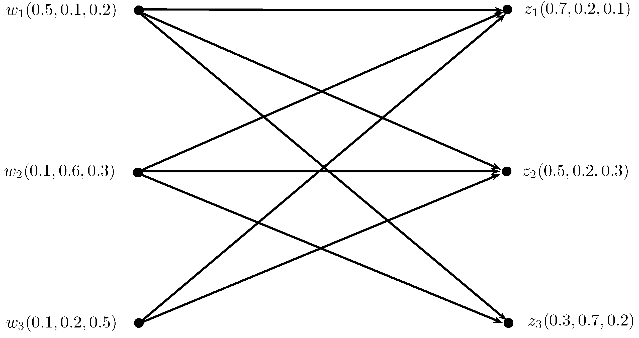
Example 2.
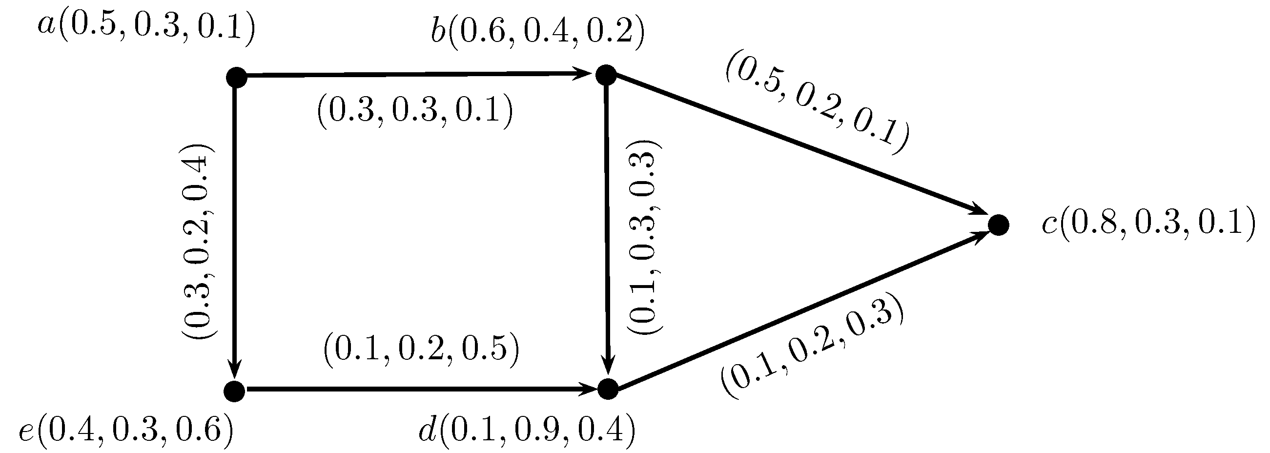
Consider , h, to be an IN-digraph, such that, , b, c, d, , a, , , , (b, , , , (c, , , , (d, , , , (e, , , and , , , , , , , , , , , , , , , , , , , , , , , , as shown in Figure 2.
Then, , , , , , , , , , , , , , and a, , , , b, , , , (d, , , . Similarly, we can calculate IN-out and in-neighborhoods of the remaining vertices.
Definition 7.
The height of an IN-set , , , is defined as:
For example, the height of an IN-set , , , , , , , , , , , in , b, is , , .
Definition 8.
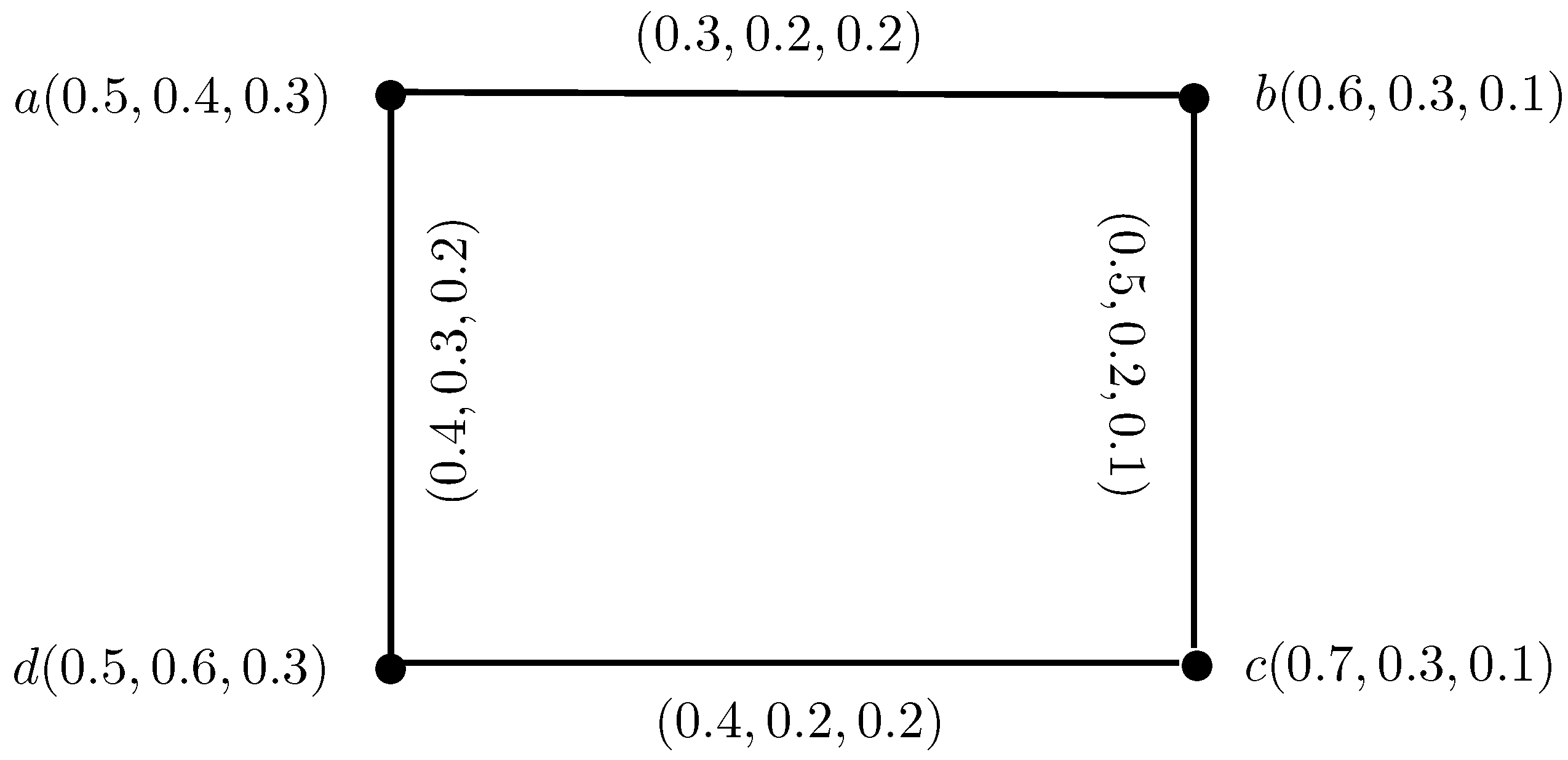
An intuitionistic neutrosophic competition graph (INC-graph) of an IN-digraph , h, is an undirected IN-graph X, h, , which has the same intuitionistic neutrosophic set of vertices as in and has an intuitionistic neutrosophic edge between two vertices w, in if and only if is a non-empty IN-set in . The truth-membership, indeterminacy-membership and falsity-membership values of edge , in are:
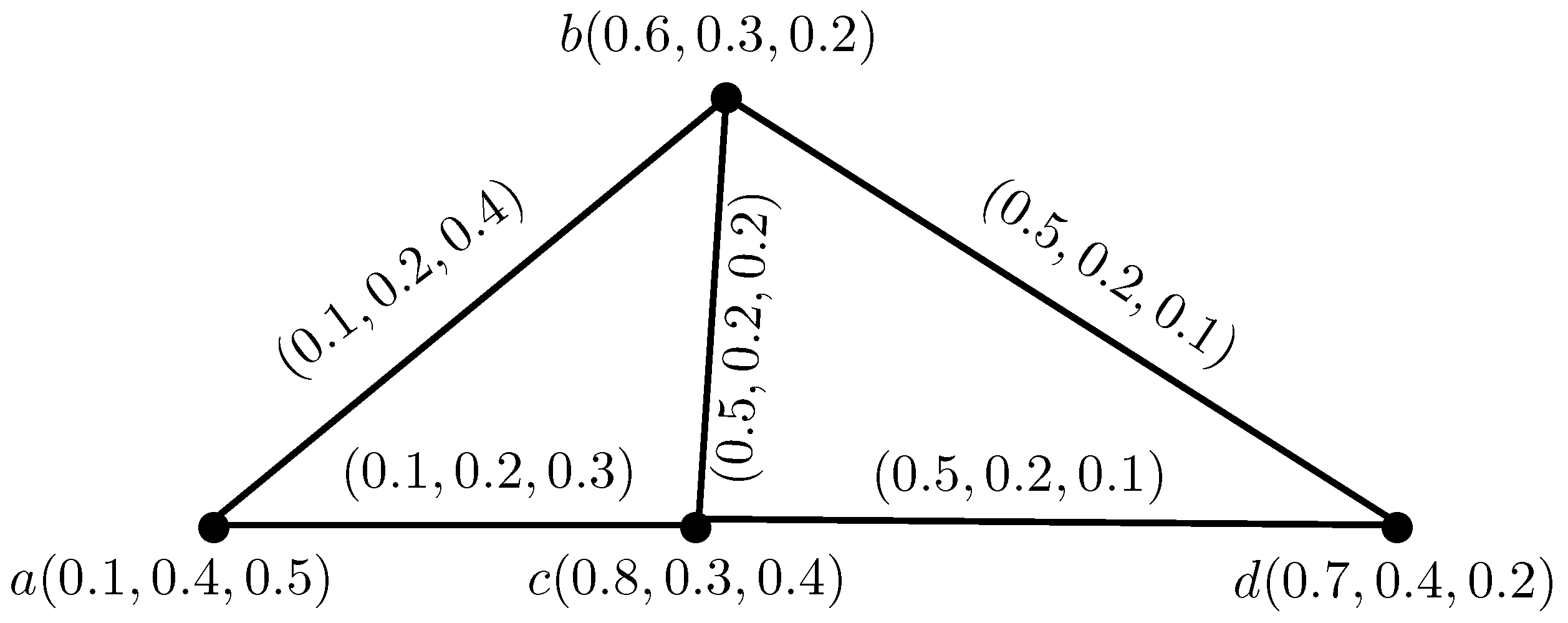
Example 3.
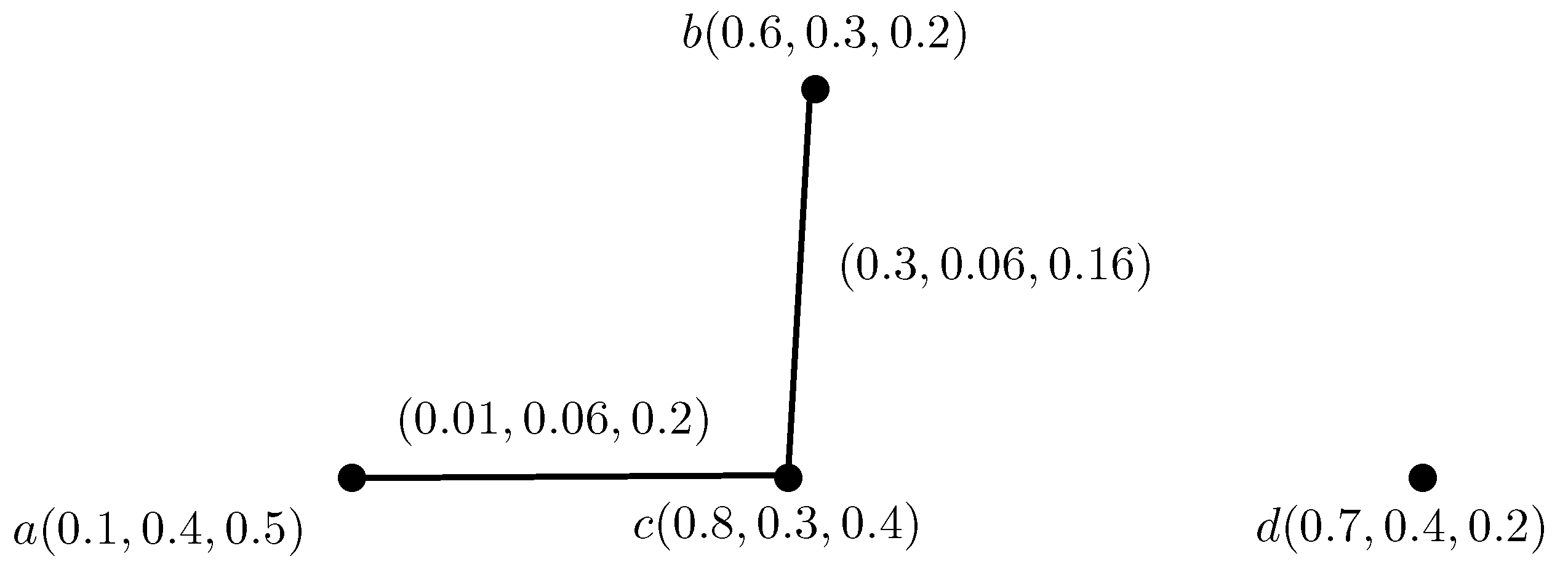
Consider , h, to be an IN-digraph, such that, , b, c, , , , , , , , , , , , , , , , , and , , , , , , , , , , , , , , , , , , , , as shown in Figure 3.
By direct calculations, we have Table 1 and Table 2 representing IN-out and in-neighborhoods, respectively.
Therefore, there is an edge between two vertices in INC-graph , whose truth-membership, indeterminacy-membership and falsity-membership values are given by the above formula.
Definition 9.
For an IN-graph , h, , where , , and , , , then an edge , , w, z is called independent strong if:
Otherwise, it is called weak.
Theorem 1.
Suppose is an IN-digraph. If contains only one element of , then the edge , of is independent strong if and only if:
Proof.
Suppose, is an IN-digraph. Suppose , , q, , where , q and r are the truth-membership, indeterminacy-membership and falsity-membership values of either the edge , or the edge , , respectively. Here,
Then,
Therefore, the edge , in is independent strong if and only if , and . Hence, the edge , of is independent strong if and only if:
☐
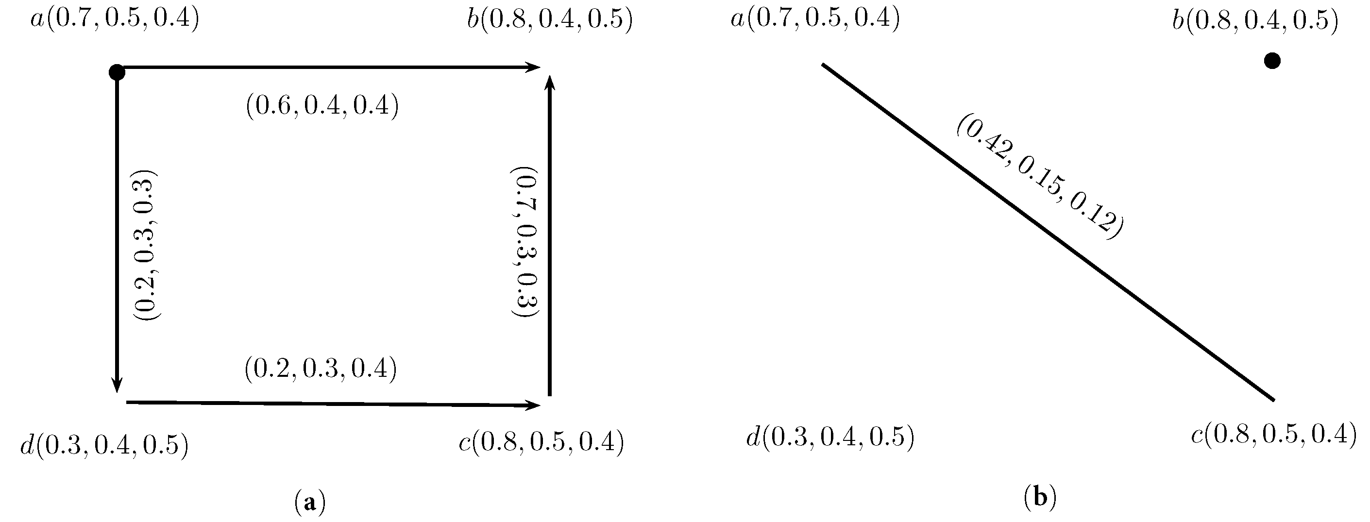
We illustrate the theorem with an example as shown in Figure 5.
Theorem 2.
If all the edges of an IN-digraph are independent strong, then:
for all edges , in .
Proof.
Suppose all the edges of IN-digraph are independent strong. Then:
for all the edges , in . Let the corresponding INC-graph be .
Case (1): When for all w, , then there does not exist any edge in between w and z. Thus, we have nothing to prove in this case.
Case (2): When , let , , , , , , , , …, , , , , where , and are the truth-membership, indeterminacy-membership and falsity-membership values of either or for , 2, …, l, respectively. Therefore,
Suppose,
Obviously, and and for all edges show that:
therefore,
and:
Hence, , , and for all edges , in . ☐
Theorem 3.
Let , and , be two INC-graph of IN-digraphs , and , , respectively. Then, where, is an IN-graph on the crisp graph , and are the crisp competition graphs of and , respectively. is an IN-graph on such that:
- 1.
- 2.
- , ,
- 3.
- 4.
- 5.
- 6.
- 7.
- 8.
- 9.
- 10.
- 11.
Proof.
Using similar arguments as in Theorem 2.1. [39], it can be proven. ☐
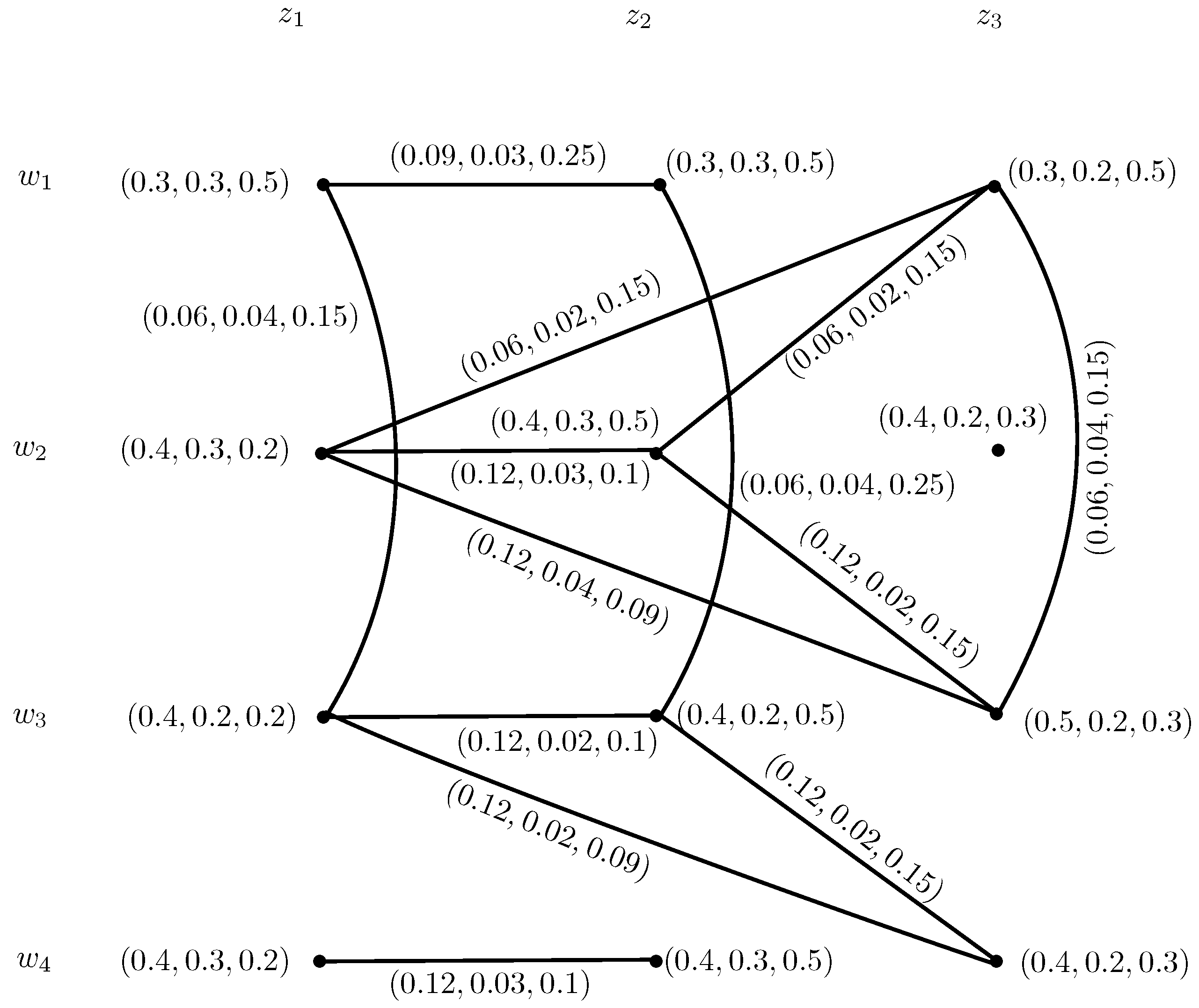
Example 4.
Consider , , and , , to be two IN-digraphs, respectively, as shown in Figure 6. The intuitionistic neutrosophic out and in-neighborhoods of and are given in Table 3 and Table 4. The INC-graphs and are given in Figure 7.
We now construct the INC-graph , , where , , and , , , from and using Theorem . We obtained two sets of edges by using Condition .
The truth-membership, indeterminacy-membership and falsity-membership of edges can be calculated by using Conditions to as,
All the truth-membership, indeterminacy-membership and falsity-membership degrees of adjacent edges of and are given in Table 5.
The INC-graph obtained by using this method is given in Figure 8 where solid lines indicate part of INC-graph obtained from , and the dotted lines indicate the part of .
Definition 10.
The intuitionistic neutrosophic open-neighborhood of a vertex w of an IN-graph , h, is IN-set , , , , where,
and defined by , , defined by , and defined by , . For every vertex , the intuitionistic neutrosophic singleton set, , , , , such that: , , defined by , and , respectively. The intuitionistic neutrosophic closed-neighborhood of a vertex w is .
Definition 11.
Suppose , h, is an IN-graph. The single-valued intuitionistic neutrosophic open-neighborhood graph of is an IN-graph , h, , which has the same intuitionistic neutrosophic set of vertices in and has an intuitionistic neutrosophic edge between two vertices w, in if and only if is a non-empty IN-set in . The truth-membership, indeterminacy-membership and falsity-membership values of the edge , are given by:
Definition 12.
Suppose , h, is an IN-graph. The single-valued intuitionistic neutrosophic closed-neighborhood graph of is an IN-graph , h, , which has the same intuitionistic neutrosophic set of vertices in and has an intuitionistic neutrosophic edge between two vertices w, in if and only if is a non-empty IN-set in . The truth-membership, indeterminacy-membership and falsity-membership values of the edge , are given by:
Example 5.
Theorem 4.
For each edge of an IN-graph , there exists an edge in .
Proof.
Suppose , is an edge of an IN-graph , h, . Suppose , h, is the corresponding closed neighborhood of an IN-graph. Suppose w, and w, . Then, w, . Hence,
Then,
Thus, for each edge , in IN-graph , there exists an edge , in . ☐
Definition 13.
The support of an IN-set , , , in X is the subset of X defined by:
and is the number of elements in the set.
We now discuss p-competition intuitionistic neutrosophic graphs.
Suppose p is a positive integer. Then, p-competition IN-graph of the IN-digraph , h, is an undirected IN-graph , h, , which has the same intuitionistic neutrosophic set of vertices as in and has an intuitionistic neutrosophic edge between two vertices w, z in if and only if . The truth-membership value of edge , in is , ; the indeterminacy-membership value of edge , in is , ; and the falsity-membership value of edge , in is , where .
The three-competition IN-graph is illustrated by the following example.
Example 6.
Consider , h, to be an IN-digraph, such that , , , , , , , , , , , , , , , , , , , , , , , , , , , , , and , , , , , , , , , , , , , , , , , , , , , , , as shown in Figure 13. Then, , , , , , , , , , , , , , , , , , , , , , , , and , , , , , , , . Therefore, , , , , , , , , , , , , , , , , , , , and , , , , , , , .
Now, . For , , , , and , . As shown in Figure 14.
We now define another extension of INC-graph known as the m-step INC-graph.
- : a directed intuitionistic neutrosophic path of length m from z to w.
- : single-valued intuitionistic neutrosophic m-step out-neighborhood of vertex z.
- : single-valued intuitionistic neutrosophic m-step in-neighborhood of vertex z.
- : m-step INC-graph of the IN-digraph .
Definition 14.
Suppose , h, is an IN-digraph. The m-step IN-digraph of is denoted by , h, where the intuitionistic neutrosophic set of vertices of is the same as the intuitionistic neutrosophic set of vertices of and has an edge between z and w in if and only if there exists an intuitionistic neutrosophic directed path in .
Definition 15.
The intuitionistic neutrosophic m-step out-neighborhood of vertex z of an IN-digraph , h, is IN-set:
there exists a directed intuitionistic neutrosophic path of length m from z to w, , , , , and , are defined by , , is an edge of , , , is an edge of and , , is an edge of , respectively.
Definition 16.
The intuitionistic neutrosophic m-step in-neighborhood of vertex z of an IN-digraph , h, is IN-set:
there exists a directed intuitionistic neutrosophic path of length m from w to z, , , , , and , are defined by , , is an edge of , , , is an edge of and , , is an edge of , respectively.
Definition 17.
Suppose , h, is an IN-digraph. The m-step INC-graph of IN-digraph is denoted by , h, , which has the same intuitionistic neutrosophic set of vertices as in and has an edge between two vertices w, in if and only if is a non-empty IN-set in . The truth-membership value of edge , in is , ; the indeterminacy-membership value of edge , in is , ; and the falsity-membership value of edge , in is , .
The two-step INC-graph is illustrated by the following example.
Example 7.
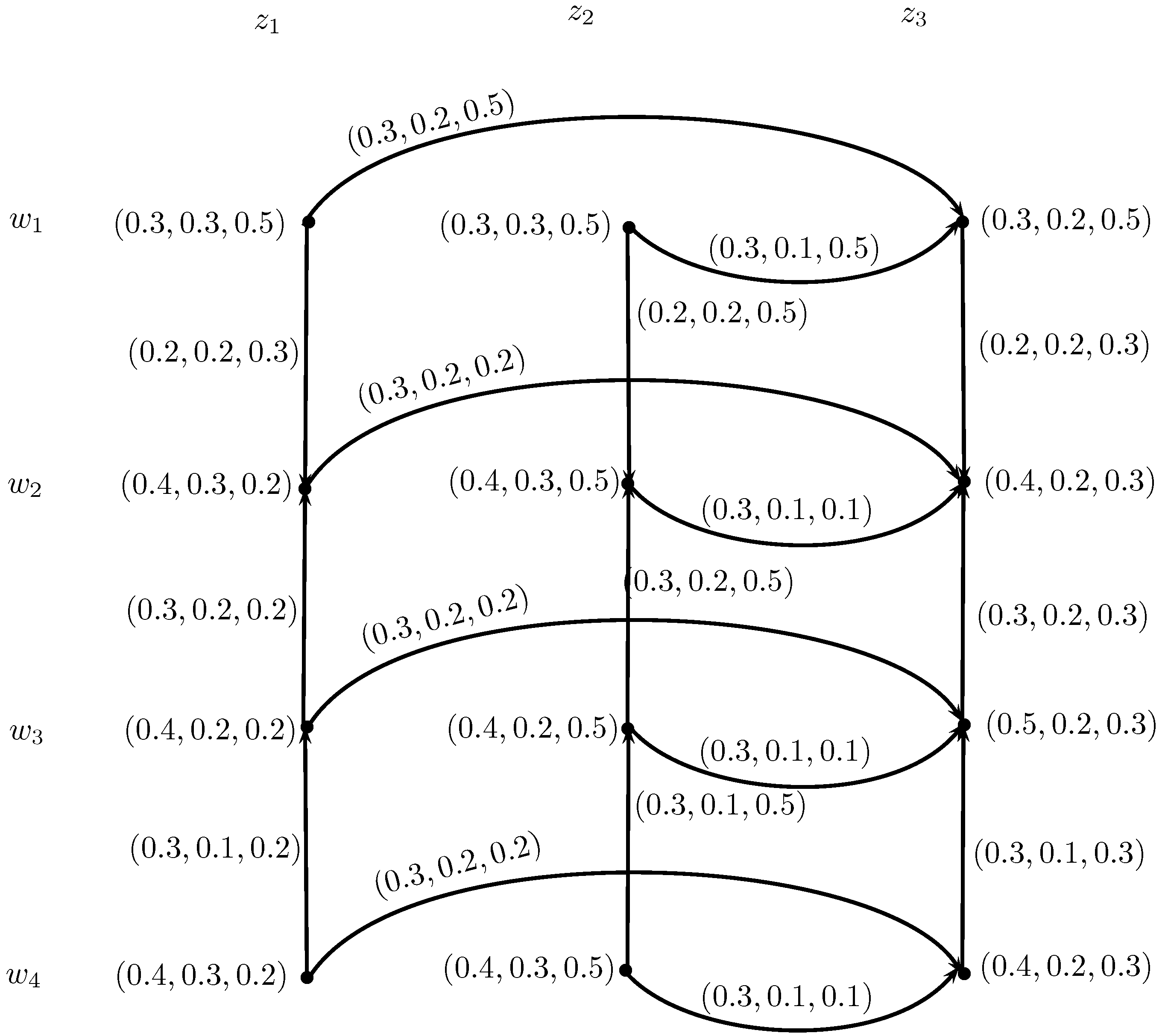
Consider , h, is an IN-digraph, such that, , , , , , , , , , , , , , , , , , , , , , , , , , , , , , and , , , , , , , , , , , , , , , , , , , , and , , , , as shown in Figure 15.
Then, , , , , , , , and , , , , , , , . Therefore, , , , , , , , . Thus, , and . This is shown in Figure 16.
Definition 18.
The intuitionistic neutrosophic m-step out-neighborhood of vertex z of an IN-digraph , h, is IN-set:
there exists a directed intuitionistic neutrosophic path of length m from z to w, , , , , and , are defined by , , , is an edge of , , , , is an edge of and , , , is an edge of , respectively.
Definition 19.
Suppose , h, is an IN-graph. Then, the m-step intuitionistic neutrosophic neighborhood graph (IN-neighborhood-graph) is defined by , h, , where , , , , , , , , , and are such that:
Theorem 5.
If all the edges of IN-digraph , h, are independent strong, then all the edges of are independent strong.
Proof.
Suppose , h, is an IN-digraph and , h, is the corresponding m-step INC-graph. Since all the edges of are independent strong, then , and . Then, , or , or , , or , or and , or , or .
Hence, the edge , is independent strong in . Since, , is taken to be the arbitrary edge of , thus all the edges of are independent strong. ☐
3. Applications
Competition graphs are very important to represent the competition between objects. However, still, these representations are unsuccessful to deal with all the competitions of world; for that purpose, INC-graphs are introduced. Now, we discuss the applications of INC-graphs to study the competition along with algorithms. The INC-graphs have many utilizations in different areas.
3.1. Ecosystem
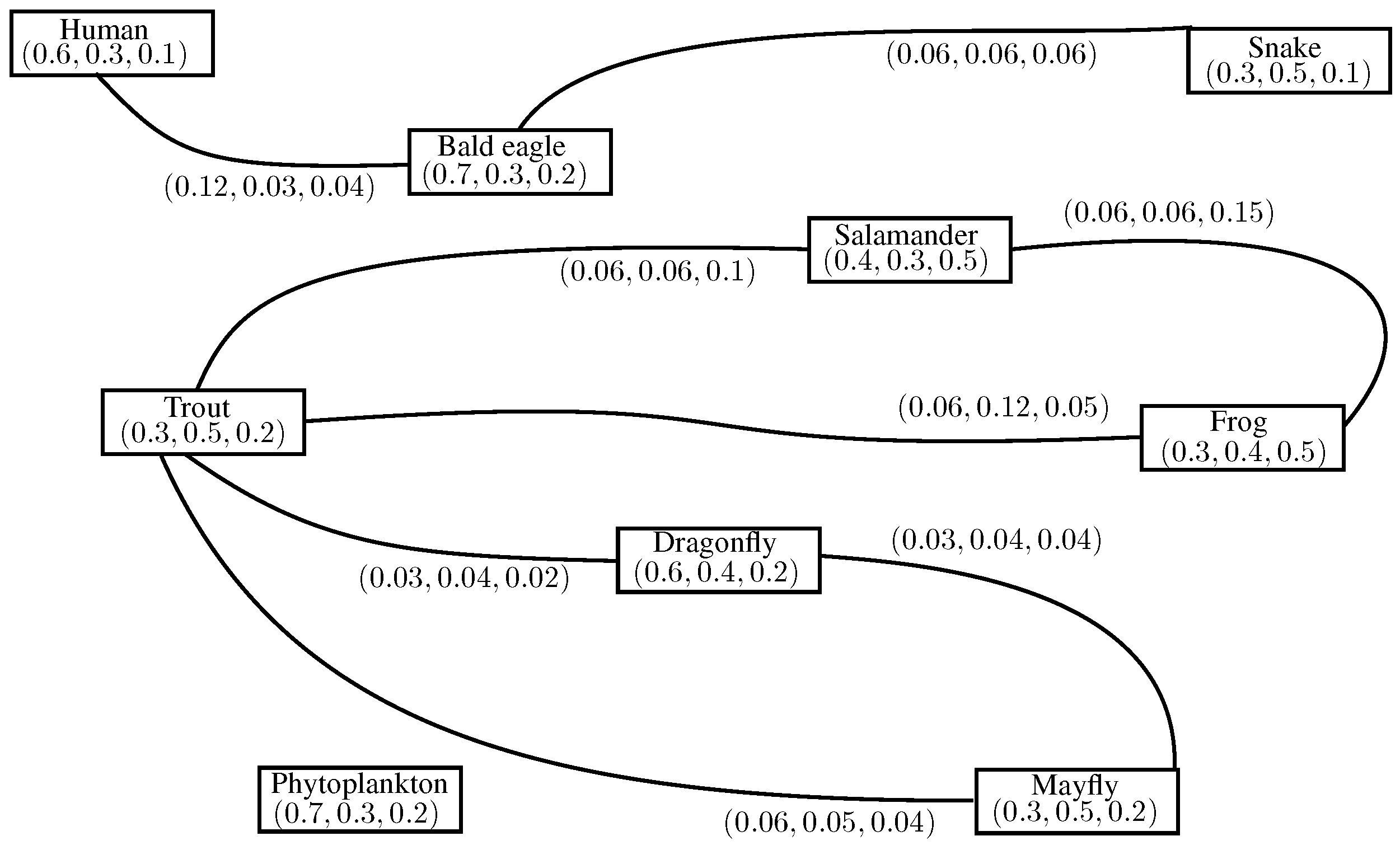
Consider a small ecosystem: human eats trout; bald eagle eats trout and salamander; trout eats phytoplankton, mayfly and dragonfly; salamander eats dragonfly and mayfly; snake eats salamander and frog; frog eats dragonfly and mayfly; mayfly eats phytoplankton; dragonfly eats phytoplankton. These nine species human, bald eagle, salamander, snake, frog, dragonfly, trout, mayfly and phytoplankton are taken as vertices. Let the degree of existence in the ecosystem of human be , the degree of indeterminacy of existence be and the degree of false-existence be , i.e., the truth-membership, indeterminacy-membership and falsity-membership values of the vertex human are , , . Similarly, we assume the truth-membership, indeterminacy-membership and falsity-membership values of other vertices as , , , , , , , , , , , , , , , , , , , , and , , . Suppose that human likes to eat trout , indeterminate to eat and dislike to eat, say . The likeness, indeterminacy and dislikeness of preys for predators are shown in Table 7.
It is clear that if trout is removed from the food cycle, then human must be lifeless, and in such a situation bald eagle, phytoplankton, dragonfly and mayfly grow in an undisciplined manner. Thus, we can evaluate the food cycle with the help of INC-graphs.
Therefore, , , , , , , , , , , , , , , , , , , , , , , , , , , , , , , , , , , , , , , , and , , , .
Now, there is an edge between human and bald eagle; snake and bald eagle; salamander and trout; salamander and frog; trout and frog; trout and dragonfly; trout and mayfly; dragonfly and mayfly in the INC-graph, which highlights the competition between them; and for the other pair of species, there is no edge, which indicates that there is no competition in the INC-graph Figure 18. For example, there is an edge between human and bald eagle indicating a degree of likeness to prey on the same species, a degree of indeterminacy and a degree of non-likeness between them.
We present our method, which is used in our ecosystem application in Algorithm 1.
| Algorithm 1: Ecosystem. |
|
3.2. Career Competition
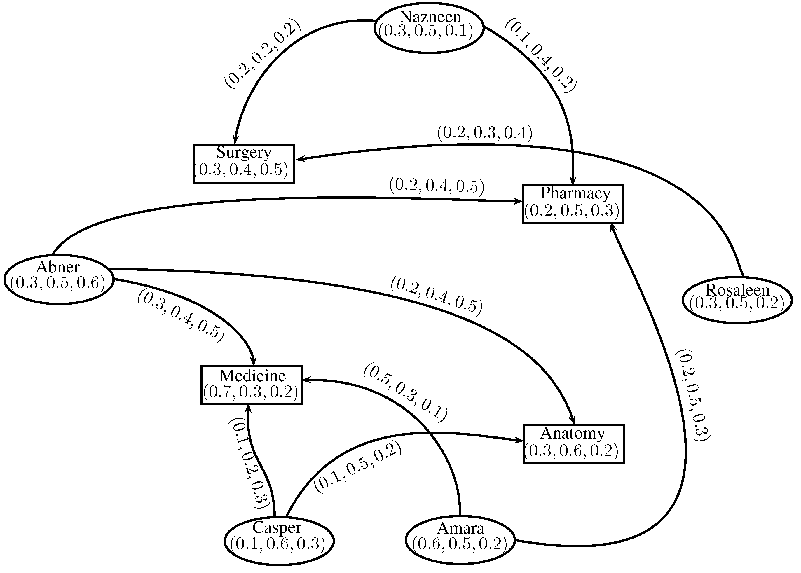
Consider the IN-digraph Figure 19 representing the competition between applicants for a career. Let , , , , be the set of applicants for the particular careers , , , . The truth-membership value of each applicant represents the degree of loyalty quality; the indeterminacy-value represents the indeterminate state of loyalty; and the false-membership value represents the disloyalty of each applicant towards their careers. Let the degree of truth-membership of Nazneen of her loyalty towards her career be : degree of indeterminacy is , and degree of disloyalty is , i.e., the truth-membership, indeterminacy and falsity-membership values of the vertex Nazneen are , , . The truth-membership value of each directed edge between an applicant and a career represents the eligibility for that career; the indeterminacy-value represents the indeterminate state of that career; and the false-membership value represents non-eligibility for that particular career.
Thus, in Table 9, , , , , , , , , , , , , , , , , , , , , , , , , , , , and , , , , , , , .
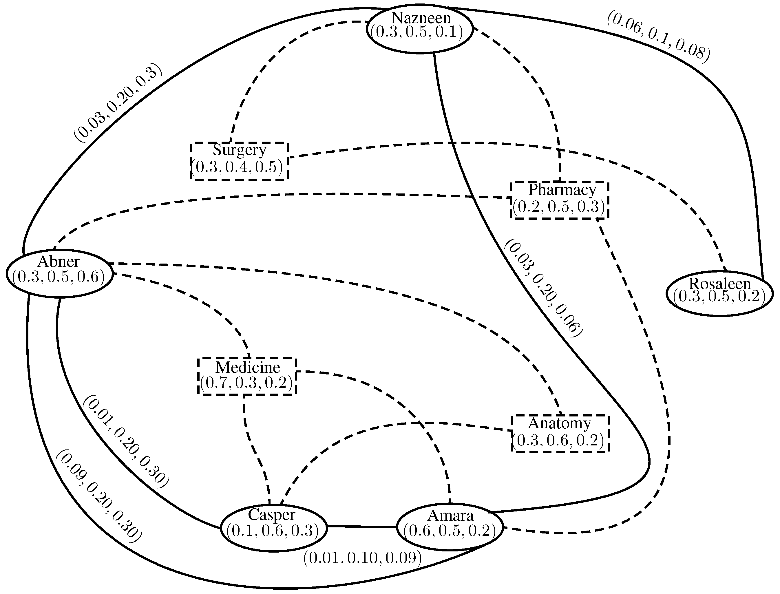
The INC-graph is shown in Figure 20. The solids lines indicate the strength of competition between two applicants, and dashed lines indicate the applicant competing for the particular career. For example, Nazneen and Rosaleen both are competing for the career, surgery, and the strength of competition between them is , , . In Table 10, , represents the competition of applicant z for career c with respect to loyalty quality, indeterminacy and disloyalty to compete with the others. The strength to compete with the other applicants with respect to a particular career is calculated in Table 10.
From Table 10, Nazneen and Rosaleen have equal strength to compete with the other for the career, surgery. Abner and Casper have equal strength of competition for the career, anatomy. Amara competes with the others for the career, pharmacy and medicine.
We present our method, which is used in our career competition application in Algorithm 2.
| Algorithm 2: Career Competition |
|
4. Conclusions
Graphs serve as mathematical models to analyze many concrete real-world problems successfully. Certain problems in physics, chemistry, communication science, computer technology, sociology and linguistics can be formulated as problems in graph theory. Intuitionistic neutrosophic set theory is a mathematical tool to deal with incomplete and vague information. Intuitionistic neutrosophic set theory deals with the problem of how to understand and manipulate imperfect knowledge. In this research paper, we have described the concept of intuitionistic neutrosophic competition graphs. We have also presented applications of intuitionistic neutrosophic competition graphs in ecosystem and career competition. We aim to extend our research work of fuzzification to (1) fuzzy soft competition graphs, (2) fuzzy rough soft competition graphs, (3) bipolar fuzzy soft competition graphs and (4) the application of fuzzy soft competition graphs in decision support systems.
Author Contributions
Muhammad Akram and Maryam Nasir conceived and designed the experiments; Maryam Nasir performed the experiments; Muhammad Akram and Maryam Nasir analyzed the data; Maryam Nasir contributed reagents/materials/analysis tools; Muhammad Akram wrote the paper.
Conflicts of Interest
The authors declare that they have no conflict of interest regarding the publication of this research article.
References
- Euler, L. Solutio problems ad geometriam situs pertinentis. Comment. Acad. Sci. Imp. Petropolitanae 1736, 8, 128–140. (In Latin) [Google Scholar]
- Marcialis, G.L.; Roli, F.; Serrau, A. Graph Based and Structural Methods for Fingerprint Classification; Springer: Berlin/Heidelberg, Germany, 2007. [Google Scholar]
- Mordeson, J.N.; Nair, P.S. Fuzzy Graphs and Fuzzy Hypergraphs 1998, 2nd ed.; Physica Verlag: Berlin/Heidelberg, Germany, 2001. [Google Scholar]
- Schenker, A.; Last, M.; Banke, H.; Andel, A. Clustering of Web Documents Using a Graph Model; Springer: Berlin/Heidelberg, Germany, 2007. [Google Scholar]
- Shirinivas, S.G.; Vetrivel, S.; Elango, N.M. Applications of graph theory in computer science an overview. Int. J. Eng. Sci. Technol. 2010, 2, 4610–4621. [Google Scholar]
- Cohen, J.E. Interval Graphs and Food Webs: A Finding and a Problems; Document 17696-PR; RAND Corporation: Santa Monica, CA, USA, 1968. [Google Scholar]
- Smarandache, F. Neutrosophic set-a generalization of the intuitionistic fuzzy set. In Proceedings of the IEEE International Conference Granular Computing, Atlanta, GA, USA, 10–12 May 2006; pp. 38–42. [Google Scholar]
- Smarandache, F. Neutrosophy. Neutrosophic Probability, Set, and Logic, ProQuest Information & Learning; InfoLearnQuest: Ann Arbor, MI, USA, 1998. [Google Scholar]
- Wang, H.; Smarandache, F.; Zhang, Y.; Sunderraman, R. Single valued neutrosophic sets. Multisapace Multistruct. 2010, 4, 410–413. [Google Scholar]
- Yang, H.-L.; Guo, Z.-L.; She, Y.; Liao, X. On single valued neutrosophic relations. J. Intell. Fuzzy Syst. 2016, 30, 1045–1056. [Google Scholar]
- Bhowmik, M.; Pal, M. Intuitionistic neutrosophic set. J. Inf. Comput. Sci. 2009, 4, 142–152. [Google Scholar]
- Bhowmik, M.; Pal, M. Intuitionistic neutrosophic set relations and some of its properties. J. Inf. Comput. Sci. 2010, 5, 183–192. [Google Scholar]
- Kauffman, A. Introduction a La Theorie Des Sousemsembles Flous; Masson: Paris, France, 1973. (In French) [Google Scholar]
- Rosenfeld, A. Fuzzy graphs. In Fuzzy Sets and their Application; Zadeh, L.A., Fu, K.S., Shimura, M., Eds.; Academic Press: New York, NY, USA, 1975; pp. 77–95. [Google Scholar]
- Bhattacharya, P. Some remark on fuzzy graphs. Pattern Recognit. Lett. 1987, 6, 297–302. [Google Scholar]
- Akram, M.; Davvaz, B. Strong intuitionistic fuzzy graphs. Filomat 2012, 26, 177–196. [Google Scholar]
- Akram, M.; Dudek, W.A. Intuitionistic fuzzy hypergraphs with applications. Inf. Sci. 2013, 218, 182–193. [Google Scholar]
- Akram, M.; Al-Shehrie, N.O. Intuitionistic fuzzy cycles and intuitionistic fuzzy trees. Sci. World J. 2014, 7, 654–661. [Google Scholar]
- Akram, M.; Siddique, S. Neutrosophic competition graphs with applications. J. Intell. Fuzzy Syst. 2017, 33, 921–935. [Google Scholar] [CrossRef]
- Akram, M.; Luqman, A. Bipolar neutrosophic hypergraphs with applications. J. Intell. Fuzzy Syst. 2017, 33, 1699–1713. [Google Scholar]
- Al-Shehrie, N.O.; Akram, M. Bipolar fuzzy competition graphs. Ars Comb. 2015, 121, 385–402. [Google Scholar]
- Sahoo, S.; Pal, M. Intuitionistic fuzzy competition graphs. J. Appl. Math. Comput. Sci. 2016, 52, 37–57. [Google Scholar]
- Smarandache, F. Types of Neutrosophic Graphs and Neutrosophic Algebraic Structures together with Their Applications in Technology Seminar; Universitatea Transilvania din Brasov, Facultatea de Design de Produs si Mediu: Brasov, Romania, 2015. [Google Scholar]
- Wu, S.Y. The compositions of fuzzy digraphs. J. Res. Educ. Sci. 1986, 31, 603–628. [Google Scholar]
- Samanta, S.; Pal, M. Fuzzy k-competition and p-competition graphs. Fuzzy Inf. Eng. 2013, 2, 191–204. [Google Scholar]
- Samanta, S.; Akram, M.; Pal, M. m-step fuzzy competition graphs. J. Appl. Math. Comput. 2015, 47, 461–472. [Google Scholar]
- Dhavaseelan, R.; Vikramaprasad, R.; Krishnaraj, V. Certain types of neutrosophic graphs. Int. J. Math. Sci. Appl. 2015, 5, 333–339. [Google Scholar]
- Akram, M.; Shahzadi, G. Operations on single-valued neutrosophic graphs. J. Uncertain Syst. 2017, 11, 176–196. [Google Scholar]
- Akram, M.; Shahzadi, S. Neutrosophic soft graphs with application. J. Intell. Fuzzy Syst. 2017, 32, 841–858. [Google Scholar]
- Broumi, S.; Talea, M.; Bakali, A.; Smarandache, F. Single valued neutrosophic graphs. J. New Theory 2016, 10, 86–101. [Google Scholar]
- Ye, J. Single-valued neutrosophic minimum spanning tree and its clustering method. J. Intell. Syst. 2014, 23, 311–324. [Google Scholar]
- Ye, J. Improved correlation coefficients of single-valued neutrosophic sets and interval neutrosophic sets for multiple attribute decision making. J. Intell. Fuzzy Syst. 2014, 27, 2453–2462. [Google Scholar]
- Ye, J. A multicriteria decision-making method using aggregation operators for simplified neutrosophic sets. J. Intell. Fuzzy Syst. 2014, 26, 2459–2466. [Google Scholar]
- Atanassov, K.T. Intuitionistic fuzzy sets. VII ITKR’s Session, Deposited in Central for Sciences Technical Library of Bulgarian Academy of Science, 1697/84, Sofia, Bulgaria 1983. Int. J. Bioautom. 2016, 20, S1–S6. [Google Scholar]
- Liang, R.; Wang, J.; Li, L. Multi-criteria group decision making method based on interdependent inputs of single valued trapezoidal neutrosophic information. Neural Comput. Appl. 2016. [Google Scholar] [CrossRef]
- Liang, R.; Wang, J.; Zhang, H. A multi-criteria decision-making method based on single-valued trapezoidal neutrosophic preference relations with complete weight information. Neural Comput. Appl. 2017. [Google Scholar] [CrossRef]
- Lundgren, J.R.; Maybee, J.S. Food Webs With Interval Competition Graph. In Graphs and Application, Proceedings of the First Colorado Symposium on Graph Theory; Wiley: New York, NY, USA, 1984. [Google Scholar]
- Mondal, T.K.; Samanta, S.K. Generalized intuitionistic fuzzy sets. J. Fuzzy Math. 2002, 10, 839–862. [Google Scholar]
- Nasir, M.; Siddique, S.; Akram, M. Novel properties of intuitionistic fuzzy competition graphs. J. Uncertain Syst. 2017, 2, 49–67. [Google Scholar]
- Peng, H.; Zhang, H.; Wang, J. Probability multi-valued neutrosophic sets and its application in multi-criteria group decision-making problems. Neural Comput. Appl. 2016. [Google Scholar] [CrossRef]
- Sarwar, M.; Akram, M. Novel concepts of bipolar fuzzy competition graphs. J. Appl. Math. Comput. 2017, 54, 511–547. [Google Scholar]
- Tian, Z.; Wang, J.; Wang, J.; Zhang, H. Simplified neutrosophic linguistic multi-criteria group decision-making approach to green product development. Group Decis. Negot. 2017, 26, 597–627. [Google Scholar] [CrossRef]
- Wang, H.; Madiraju, P.; Zang, Y.; Sunderramn, R. Interval neutrosophic sets. Int. J. Appl. Math. Stat. 2005, 3, 1–18. [Google Scholar]
- Zadeh, L.A. Fuzzy sets. Inf. Control 1965, 8, 338–353. [Google Scholar]
Figure 1.
Intuitionistic neutrosophic graph (IN-graph).

Figure 2.
IN-digraph.

Figure 3.
IN-digraph.
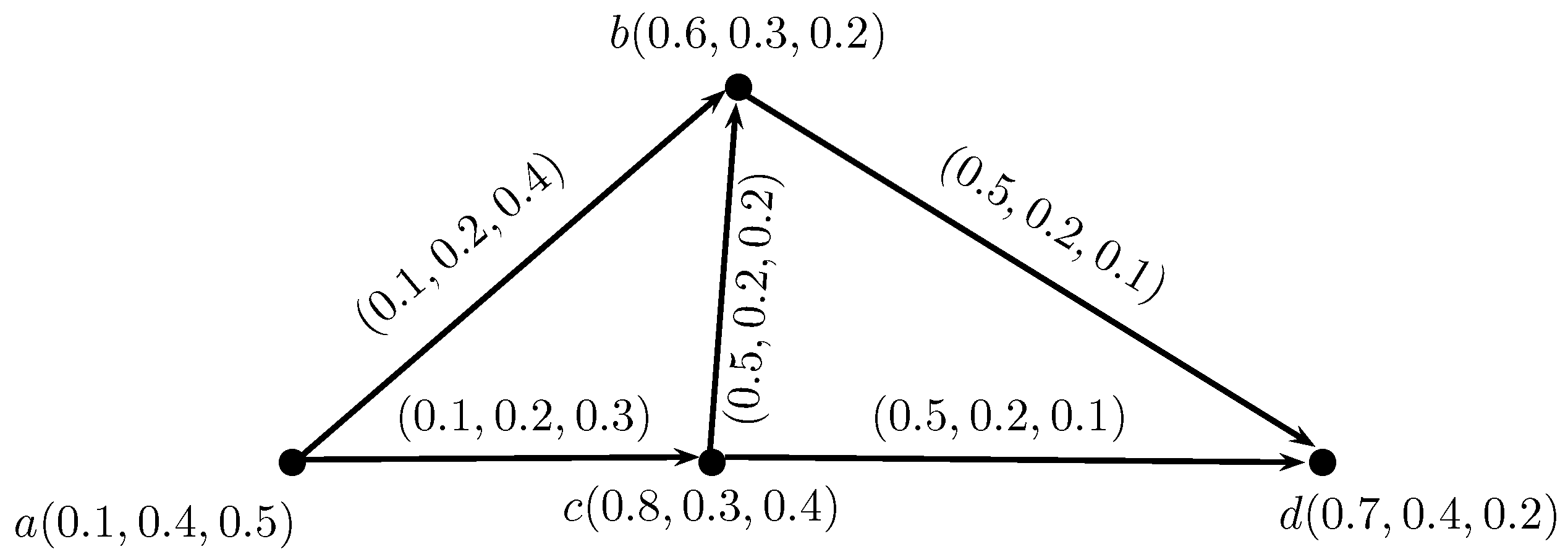
Figure 4.
Intuitionistic neutrosophic competition graph (INC-graph).

Figure 5.
INC-graph. (a) IN-digraph; (b) corresponding INC-graph.

Figure 6.
IN-digraphs.
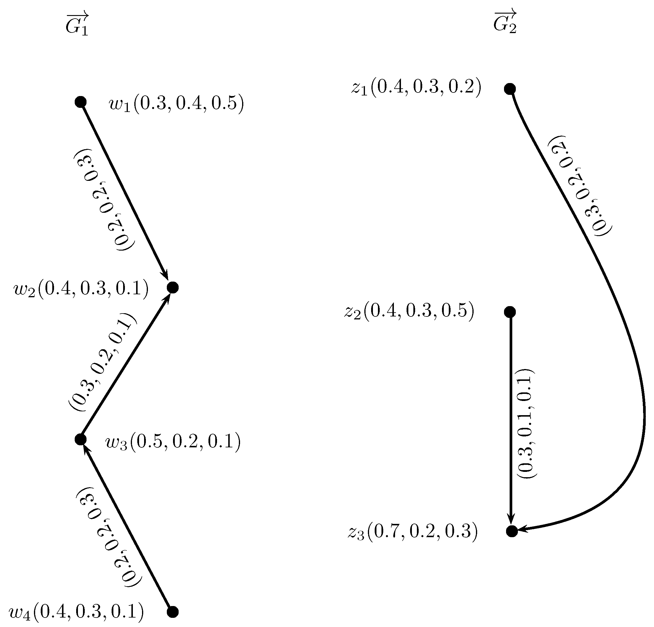
Figure 7.
INC-graphs of and .
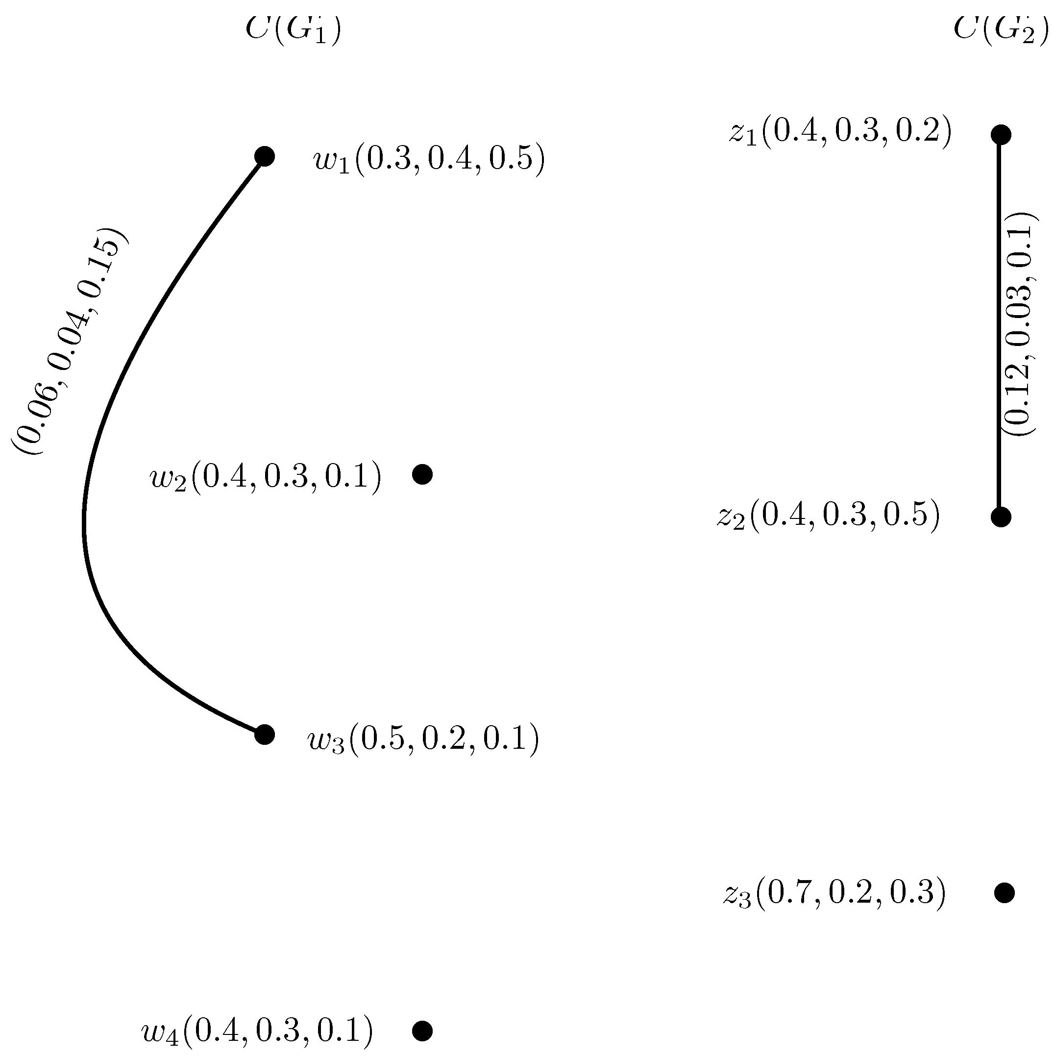
Figure 8.
∪.
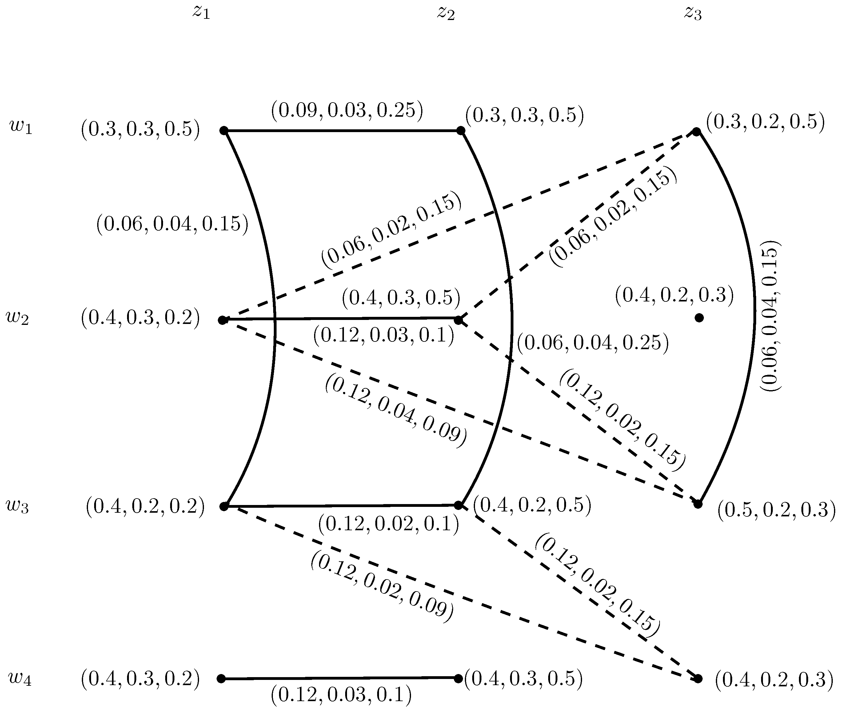
Figure 9.
.

Figure 10.
.

Figure 11.
IN-digraph.

Figure 12.
; .

Figure 13.
IN-digraph.

Figure 14.
Three-competition IN-graph.
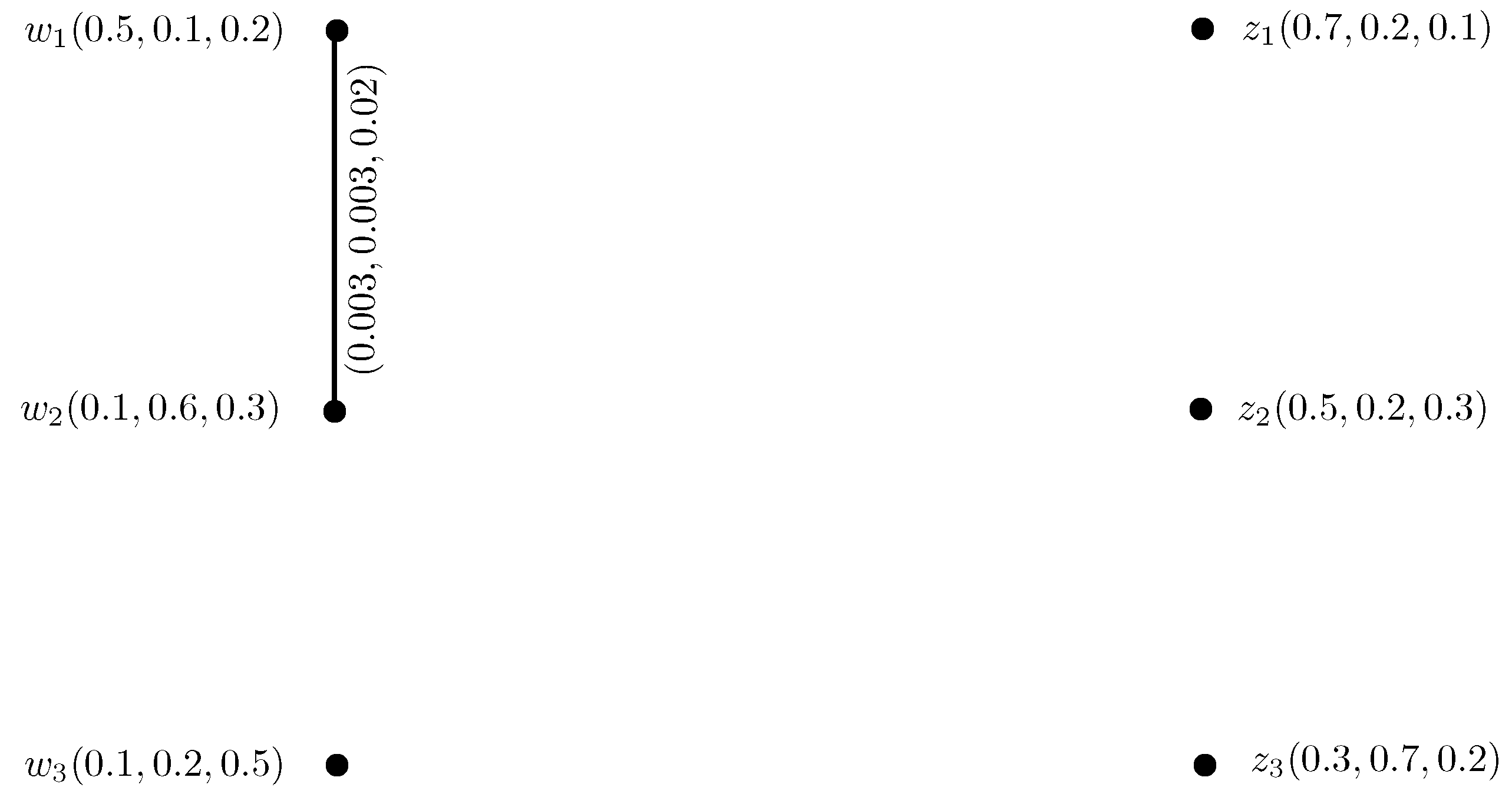
Figure 15.
IN-digraph.
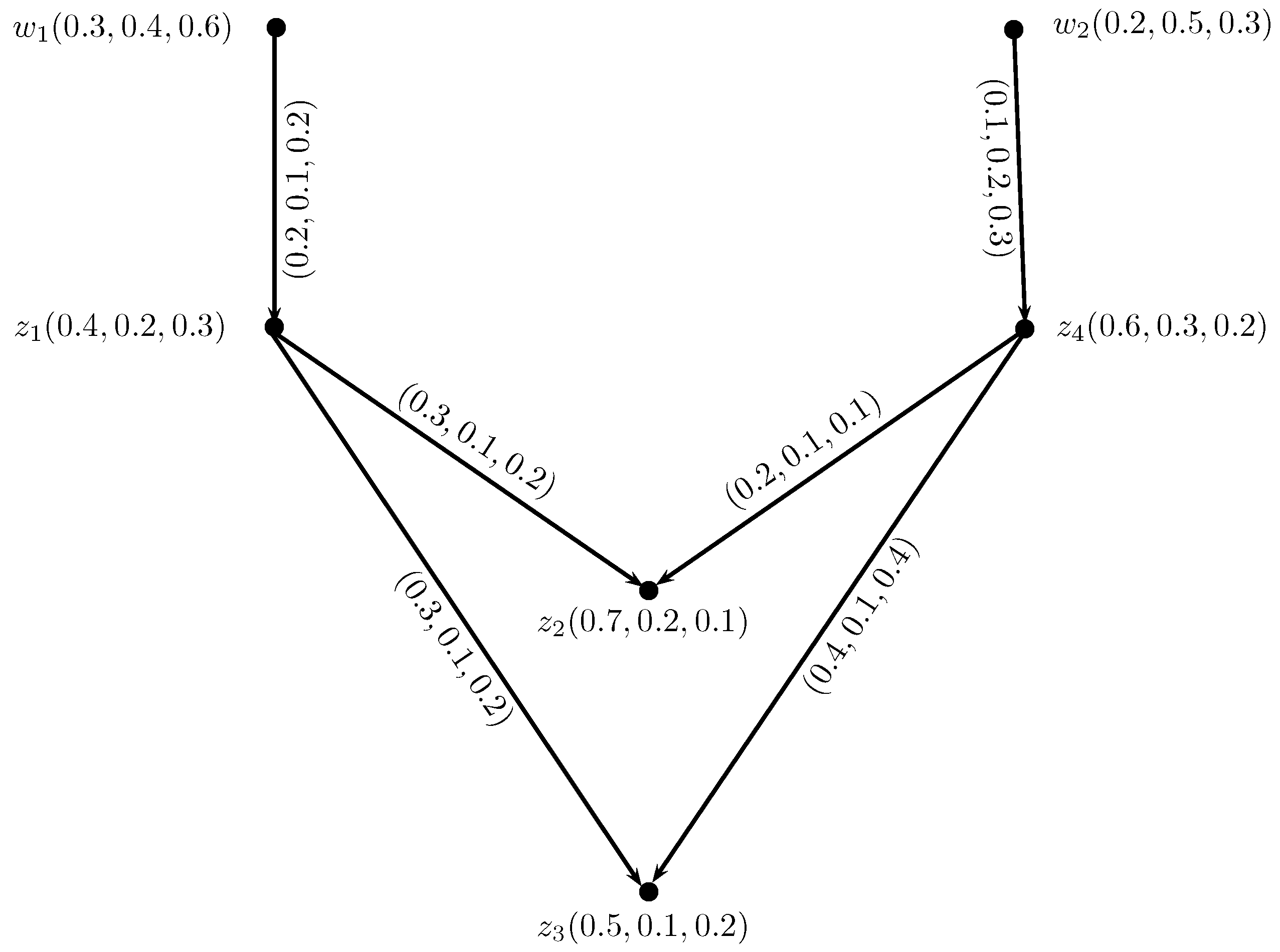
Figure 16.
Two-step INC-graph.

Figure 17.
IN-food web.
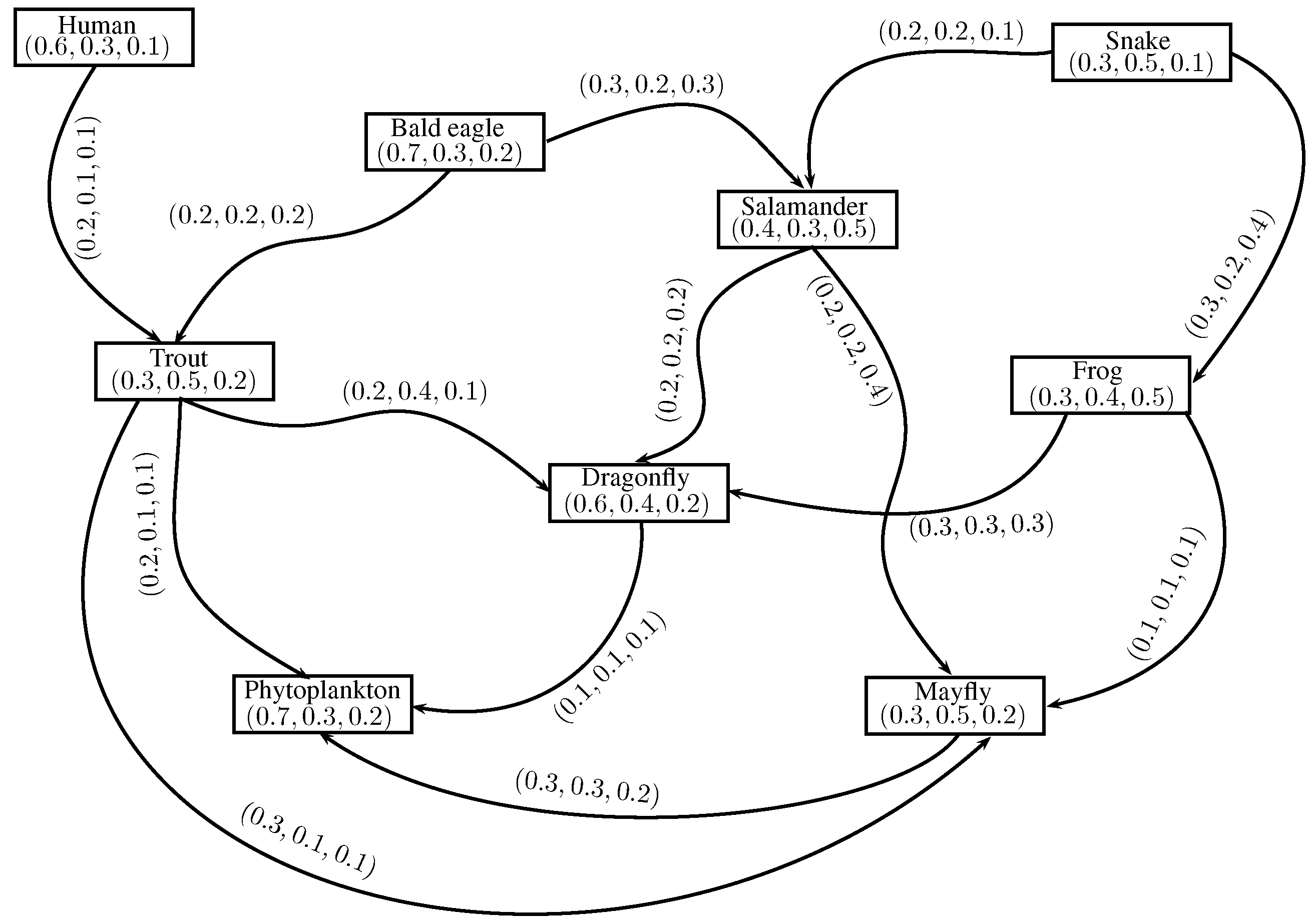
Figure 18.
Corresponding INC-graph

Figure 19.
IN-digraph.

Figure 20.
Corresponding INC-graph.


Table 1.
IN-out-neighborhoods.
| w | |
|---|---|
| a | {(b, 0.1, 0.2, 0.4), (c, 0.1, 0.2, 0.3)} |
| b | {(d, 0.5, 0.2, 0.1)} |
| c | {(b, 0.5, 0.2, 0.2), (d, 0.5, 0.2, 0.1)} |
| d | ∅ |
Table 2.
IN-in-neighborhoods.
| w | |
|---|---|
| a | ∅ |
| b | {(a, 0.1, 0.2, 0.4), (c, 0.1, 0.2, 0.3)} |
| c | {(a, 0.1, 0.2, 0.3)} |
| d | {(b, 0.5, 0.2, 0.1), (c, 0.5, 0.2, 0.1)} |
Table 3.
IN-out and in-neighborhoods of .
| ∅ | ||
| ∅ | ||
| ∅ |
Table 4.
IN-out and in-neighborhoods of .
| ∅ | ||
| ∅ | ||
| ∅ |
Table 5.
Adjacent edges of ∪.
| (, ) (, ) | k (, ) (, ) |
|---|---|
| , , | , , |
| , , | , , |
| , , | , , |
| , , | , , |
| , , | , , |
| , , | , , |
| , , | , , |
| , , | , , |
| , , | , , |
| , , | , , |
| , , | , , |
| , , | , , |
| , , | , , |
Table 6.
IN-out-neighborhoods of .
| , | , |
|---|---|
| , | , , , , , , |
| , | , , , , , , |
| , | , 0.2, , |
| , | , 0.3, , |
| , | , 0.3, , |
| , | ∅ |
| , | , , , , , , |
| , | , , , , , , |
| , | , 0.3, , |
| , | , , , , , , |
| , | , , , , , , |
| , | , 0.3, , |
Table 7.
Likeness, indeterminacy and dislikeness of preys and predators.
| Name of Predator | Name of Prey | Like to Eat | Indeterminate to Eat | Dislike to Eat |
|---|---|---|---|---|
| 20 | 10 | 10 | ||
| 20 | 20 | 20 | ||
| 30 | 20 | 30 | ||
| 20 | 20 | 10 | ||
| 30 | 20 | 40 | ||
| 20 | 20 | 20 | ||
| 20 | 20 | 40 | ||
| 30 | 30 | 30 | ||
| 20 | 40 | 10 | ||
| 30 | 10 | 10 | ||
| 20 | 10 | 10 | ||
| 10 | 10 | 10 | ||
| 30 | 30 | 20 | ||
| 10 | 10 | 10 |
Table 8.
IN-out-neighborhoods.
| , , , | |
| , , , , , , , | |
| , , , , , , , | |
| , , , , , , , | |
| , , , , , , , | |
| , , , | |
| ∅ | |
| , , , | |
| , , , , , , , , , , |
Table 9.
IN-out-neighborhoods.
| , , , , , , , | |
| , , , | |
| , , , , , , , | |
| , , , , , , , | |
| , , , , , , , , , , , |
Table 10.
Strength of competition of the applicant for a particular career.
| , | , | , | |
|---|---|---|---|
| , | , , | ||
| , | , , | ||
| , | , , | ||
| , | , , | ||
| , | , | , , | |
| , | , | , , | |
| , | , | , , | |
| , | , | , , | |
| , | , | , , | 0.665 |
| , | , | , , |
© 2017 by the authors. Licensee MDPI, Basel, Switzerland. This article is an open access article distributed under the terms and conditions of the Creative Commons Attribution (CC BY) license (http://creativecommons.org/licenses/by/4.0/).
Share and Cite
MDPI and ACS Style
Akram, M.; Nasir, M. Certain Competition Graphs Based on Intuitionistic Neutrosophic Environment. Information 2017, 8, 132. https://doi.org/10.3390/info8040132
AMA Style
Akram M, Nasir M. Certain Competition Graphs Based on Intuitionistic Neutrosophic Environment. Information. 2017; 8(4):132. https://doi.org/10.3390/info8040132
Chicago/Turabian StyleAkram, Muhammad, and Maryam Nasir. 2017. "Certain Competition Graphs Based on Intuitionistic Neutrosophic Environment" Information 8, no. 4: 132. https://doi.org/10.3390/info8040132
Note that from the first issue of 2016, this journal uses article numbers instead of page numbers. See further details here.