
Aesthetic Local Search of Wind Farm Layouts


Department of Computer Science, University of Waikato, Hamilton 3216, New Zealand
*
Author to whom correspondence should be addressed.
Information 2017, 8(2), 39; https://doi.org/10.3390/info8020039
Submission received: 12 January 2017
/
Revised: 21 February 2017
/
Accepted: 21 March 2017
/
Published: 24 March 2017
(This article belongs to the Section Information Processes)
Abstract
:The visual impact of wind farm layouts has seen little consideration in the literature on the wind farm layout optimisation problem to date. Most existing algorithms focus on optimising layouts for power or the cost of energy alone. In this paper, we consider the geometry of wind farm layouts and whether it is possible to bi-optimise a layout for both energy efficiency and the degree of visual impact that the layout exhibits. We develop a novel optimisation approach for solving the problem which measures mathematically the degree of visual impact of a layout. The approach draws inspiration from the field of architecture. To evaluate our ideas, we demonstrate them on three benchmark problems for the wind farm layout optimisation problem in conjunction with two recently-published stochastic local search algorithms. Optimal patterned layouts are shown to be very close in terms of energy efficiency to optimal non-patterned layouts.
1. Introduction
Worldwide, renewable energy production via wind is becoming increasingly important. Forecasts are that by 2030, approximately 18% of the planet’s total energy production will be sourced from wind farms [1]. The rapid growth in wind energy production is illustrated by examining some of current and planned wind farm installations around the world: the London Array [2], for example, generates 630 MW of power (enough for 490,000 households); similarly, the ongoing Gansu project in China [3] is planned to generate 20 GW by 2020 (equating to power for approximately 15 million households).
Concerns about the environmental impact of wind energy have also been increasing alongside growth in its production. In particular, it has been noted for some time that wind turbines have considerable impact on local wildlife populations, such as birds, bats and, for offshore farms, various marine wildlife [4]. Therefore, there have been recent calls for entirely new research programs to be developed solely to study the effects of wind generation on wildlife and how to mitigate [5].
The human impact of wind energy production is also considerable: wind farms tend to generate significant noise, and they have a major visual impact on the landscape due to the size of the turbines. On clear days, turbines can be seen up to 30 km away depending on the turbine height and terrain conditions [4]. Moreover, the human impact can range in severity from a “mere” belief (strong or otherwise) that wind turbines detract from the visual value of the landscape, to shadow flicker, a phenomenon caused by the interaction of a wind turbine’s blades with direct sunlight. Such a phenomenon is known to cause severe headaches when nearby residents are exposed to it for a long period [6].
This paper concerns itself with one aspect of the environmental impact of wind farm design, specifically the arrangement of wind turbines into geometrical patterns and the relationship of these geometric patterns with the overall energy efficiency of the farm.
To partially mitigate the negative visual impacts of wind farms, it has been noted that farms with a regular layout of turbines tend to be perceived as blending into the visual landscape in a better way than farms with an irregular layout [4]. More precisely, research by Tsoutsos et al. [7] discusses the aesthetic principles of wind farm layout design: farms have a higher aesthetic appeal either when turbines are arranged clearly into rows or when they are arranged into uniform density small clusters of 2–8 turbines, which are separated by obvious landmarks. The latter arrangement is particularly preferred when the wind farm must be integrated with agriculture.
One significant issue arising when considering the layout of turbines on a wind farm is the loss of wind energy due to the interaction between nearby turbines, a phenomenon known as the “wake effect”. Therefore, all configurations of turbines in a wind farm are not equal, and often, a computationally-expensive simulation (or an approximation thereof) is required to assess the wake effect so that it can be mitigated as much as possible. Sometimes, other objectives may also be considered (e.g., construction costs), but the commonality amongst many papers in the literature is a focus on wake effect minimisation. Examples include the seminal work in the field by Mosetti et al. [8], as well more recent works, such as that by Wagner et al. [9], Rodrigues et al. [10], Guirguis et al. [11] and Mayo et al. [12,13].
In general there is a trade-off between the geometric constraints required to minimise the negative visual impact of a wind farm and the energy output of the farm itself. A simple example would be the arrangement of turbines equidistantly around the perimeter of a circle: although a circle is a visually interesting shape, there will always be a sizeable portion of turbines (on opposite sides of the circle) that lie in each other’s wakes regardless of the predominant wind direction.
Beyond forcing turbines to be arranged into simple geometric shapes, such as circles and grids, it is not immediately clear how to define “visually-appealing” arrangements in a more general way. Most of the past and current works on wind farm layout optimisation (WFLO) tend to ignore geometric configuration, and consequently, highly optimised layouts may take on a “random scattering” appearance. This is shown in some of the figures later in this paper.
Two prior works have considered the visual aspects of layouts as part of the optimisation process (as far as the authors are aware): an excellent paper by Neubert et al. [14] in which turbines are constrained to a skewed grid and the orientation and skew of the grid is optimised; and an approach by Al-Yahyai et al. [15], in which turbines are also assigned positions on a grid, but in this case, only the grid’s orientation is optimised.
In both cases, the geometric constraints are extreme, and therefore, the optimisation problem can be solved by varying only two or one variables, respectively. Despite the limitations of these approaches, Neubert et al. show that the geometrically-constrained layouts are almost (within a few percentage points) as efficient as completely unconstrained layouts that are optimised purely for energy efficiency.
In this paper, we take a different tack. Rather than strongly constraining layouts in order to force a geometric pattern on them (as the previous authors have done), we instead add a pattern-based metric to the optimiser that assesses the quality of the pattern that the turbines form. Thus, each individual turbine’s position on the layout is still a degree of freedom, but at the same time, a poorly-arranged layout with the same energy efficiency as a well-arranged layout will score an overall worse objective value. Thus, the optimiser focuses its search towards layouts with minimal visual impact (or, alternatively, a strong aesthetic appeal).
To evaluate our novel approach, we use two stochastic local search algorithms for the WFLO problem that have recently appeared in the literature. Both approaches are combined with our novel objective function, thus producing two new approaches. The first existing approach we utilise is called the Turbine Displacement Algorithm (TDA) [9]. The second approach is our own recently-published approach known as BlockCopy [12,16].
In order to assess the geometric/pattern quality of layouts, we have utilised a pattern measure originally proposed by Salingaros [17,18]. This metric has its origin in the architectural evaluation of building facades, but has been generalised for the evaluation of any kind of symbolic pattern. Therefore, it is ideally suited for our purposes.
The pattern metric we use, as well as all other relevant technical details are described in the next section. Following that, we describe how we modify the objective function of the TDA and BlockCopy algorithms to optimise for geometric qualities. Section 4 and Section 5 describe a comprehensive evaluation of both algorithms that was performed, and finally, Section 6 concludes the paper.
We acknowledge at this point that the work undertaken here is largely focussed on the aesthetics of two-dimensional layouts. Thus, it would be applicable to situations where the wind farm is located off-shore or on a plain, but not in a situation where the farm is located on a three-dimensional terrain (e.g., along a ridge). Furthermore, adjustments would also have to be made to the proposed method if the importance of aesthetics varies across the layout. For example, an area of the farm close to a tourist attraction is likely to have much more visual impact than the part of the farm furtherest from the attraction. We address these concerns in the conclusion.
2. Technical Background
2.1. Jensen Wake Model
The Jensen far wake model, originally proposed in the mid-1980s [19,20], is the approach used this research to assess the wake interactions between turbines in a wind farm layout. Although dated, the Jensen is still used widely in the community. To illustrate, Samorani [21] describes it precisely in a recent 2013 introductory survey to the WFLO problem, and in a 2016 comparison of three kinematic far wake models and two field-based far wake models, Shakoor et al. [22] concluded that “...Jensen’s far wake model is a good choice to solve the wind farm layout optimisation problem due to its simplicity and relatively high degree of accuracy.” We therefore adopt the Jensen model for our initial investigations reported here, while acknowledging that more sophisticated models do exist that we will explore in future work.
In this section, we therefore describe briefly the Jensen far wake model. As we are using, more or less, the same notation as Samorani [21], the interested reader is referred to that publication for more specific details.
The first element required in wind farm modelling is a power curve, which describes the relationship between incoming wind speed and the power generated by a single wind turbine. This is generally dependent on the type of wind turbine being modelled, and therefore, will vary depending on the manufacturer and model. In general, however, the relationship can be modelled as a cubic function from wind speed to power between two bounding wind speeds: (i) the cut-in speed, which is the wind speed at which the turbine begins generating power; and (ii) the nominal speed, which is the wind speed at which maximum power production is reached. A final element of the power curve is the cut-out speed. This is the maximum allowable wind speed that the turbine can tolerate before shutting down to avoid damage.
Due to the variability and manufacturer dependence of different wind turbine models, we adopt in this paper the power curve used by Mosetti et al. [8] and also described by Samorani [21]:
In this power curve, wind speed u is measured in metres per second (m/s) and power in kilowatts (kW). This turbine model is somewhat dated (for example, modern turbines may produce 8–10 MW of power), but it is a well-known model frequently used in the literature; therefore, we adopt it in this paper for the purposes of reproducibility ease.
The next part of the Jensen far wake model is the modelling of the velocity deficit, i.e., the reduction in wind speed as wind passes through the blades of a turbine. This is best introduced schematically, and here, we reproduce a diagram from Samorani [21] in Figure 1.
The key elements of Figure 1 are an illustration of the initial wind speed ; the reduced wind speed at a distance x metres from the wind turbine; and the notion that the wake spreads out with a linearly-increasing radius as it gets further away from the turbine.
In fact, the radius of the spreading wake is modelled by the following equation:
where is the turbine’s radius and is the radius of the wake. This equation shows that the rate of spreading is determined by a constant , which in turn depends on two further factors: first, the height of the turbine z; and second, the surface roughness, . The function to calculate is:
Once the size of the spreading wake can be determined as a function of distance x, the degree of wind speed velocity deficit needs to be next computed. The relationship between wind speed and velocity deficit is modelled as:
where is the wind speed at a position j, which is inside the wake of a turbine at position i. The term represents the velocity deficit between positions i and j due to the turbine, and is calculated (according to Samorani [21]); thus:
where is the distance between the two points, and a, the “axial induction factor”, is defined as:
while , the “downstream rotor radius”, is calculated as:
This value is used as the input to the velocity deficit calculation (Equation (5) above) as per the model.
A key corollary of these equations is that while power increases with the cube of wind speed, velocity deficit decreases at a rate proportional to the square of the distance from a turbine. Therefore, it follows that simply finding a “windier” site should increase power production regardless of whether wake effects are minimised or not.
Next, the model also accounts for the fact that a turbine may be in the wake of not one, but many other wind turbines, at the same time. In this case, the velocity deficit calculation is more complex because the different velocity deficits must be aggregated together. This is achieved in the Jensen model by calculating the square root of the sum of the squared velocity deficits:
where is the total velocity deficit and is the set of turbines affecting the turbine at position j. Turbines are represented as points for the purposes of this set membership calculation, and therefore, they are either completely inside or outside the wake; we acknowledge that other wake models allow partial wake overlaps of the rotors, but we have followed the Samorani’s presentation of the Jensen model in this work, which treats turbines as points. As pointed out earlier by Shakoor et al [22], this should be sufficiently accurate.
The index s denotes the wind scenario, which specifies both the wind direction and the initial wind speed: both of these factors determine the wakes in which a turbine lies and therefore what the total velocity deficit will be.
Two things must be noted about the calculation of the set . Firstly, computing the wakes within which a turbine j lies for any arbitrary wind direction requires some non-trivial 2D geometric calculations. This is because the wind may blow in any direction, and therefore, wakes may expand in any direction. However, this calculation is readily computable using standard trigonometry.
Secondly, and more significantly, a routine to calculate the velocity deficit for every turbine in a layout for a single wind direction is a function with quadratic time complexity: this is because every turbine j in the layout must be compared to every other turbine in order to determine . Thus, layout evaluators can face scalability issues as the size of the layout increases.
Finally, to complete our presentation of the Jensen model, there are several constants required. Specifically, these are , the turbine radius, which we set to 20 m; z, the hub height, which is initialised to 60 m; , the surface roughness constant, which is 0.3 m; and , which is 0.88. A minimum allowable distance between turbines must also be specified, because the Jensen model is not accurate at close distances. We set this constant to three times the diameter of the rotors, namely 120 m. These constants are all as-used by Samorani [21]. We expect that other situations will require different unique values for the above parameters, since they depend on the model of wind turbine being used, as well as characteristics of the site. However, these values are good defaults for the purposes of reproducibility, and we do not expect the behaviour of the approaches that we present later to be significantly dependent on particular choices of values.
2.2. Objective Function
Once the Jensen model is completely specified, the next step is to precisely specify the objective function for the WFLO problem. There are generally many different ways of doing this depending on what optimisation is required. One approach is to simply calculate the total expected power generated by a wind farm, which must be maximised (e.g., [23]). Another approach is to calculate the expected cost of energy: take the total expected power; convert it into units of currency that would be obtained if the power were sold at market; and divide that revenue by the cost of building and maintaining the wind farm (e.g., [13]). This is an objective that must be minimised.
For this preliminary assessment of our new approach, we use a simple objective function that divides the total expected power generated by the farm with wake interference by the total hypothetical expected power that would be generated by the farm without wakes. Clearly, this ratio should result in a value between zero and one, with higher values being more desirable.
If is a wind farm layout, the objective function therefore is:
where j is a turbine’s position in the layout, and is the total velocity deficit at j. S is a set of wind scenarios; is the probability of scenario ; and is the wind speed under scenario s. It should be evident that in order compute proper expected power values.
2.3. Turbine Displacement Algorithm
The Turbine Displacement Algorithm (TDA) is a highly effective stochastic local search algorithm for the wind farm layout optimisation problem first introduced by Wagner et al. [9]. The algorithm shifts a single turbine at a time and then re-evaluates the layout to determine if the turbine move should be accepted or not.
Although initially designed to be used in conjunction with a specific wake model in order to reduce the computational complexity of layout evaluation, the algorithm is in fact competitive with other more general approaches that use different wake models. A recent evaluation by Wilson et al. [24] showed that TDA outperformed several other metaheuristic algorithms, including genetic algorithms and particle swarm optimisation. We therefore use TDA as one of the algorithms in our evaluation.
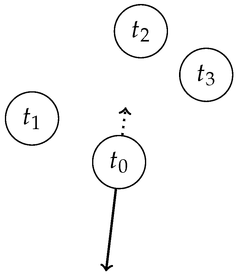
The basic behaviour of one iteration of TDA is shown in Figure 2. Essentially, a neighbourhood size K must be specified initially by the user. A random turbine is then picked, and it is moved either away from the K neighbours or, with reduced probability, towards the K neighbours. The direction that the turbine moves is called its displacement vector.
In the original paper on TDA [9], a study on the best value of K for different layout sizes was performed. It was found that for a very small layout, a small K (e.g., ) leads to an efficiency gain of just over 1% compared to higher K values; however, as the layout size increases, the difference in efficiency caused by varying K approached a negligible value. was the highest value tested in that paper.
Each displacement vector has a specific size, and one feature of the algorithm is that the size of the displacement vectors is not constant. Instead, it varies on a per-turbine basis: if a turbine’s moves are frequently accepted (i.e., lead to improvements in the objective value), then the size of that turbines displacement vector is gradually increased; conversely, if a turbine’s moves are not accepted, the size decreases.
A complete specification of TDA can be found in Wagner et al. [9], and it suffices to state the parameters that we used: the best neighbourhood size we found in initial experiments was ; the initial displacement vector size was set to 120 m; the scaling factor for reducing displacement vector sizes was 0.9, and conversely the factor for increasing sizes was ; and finally, the amount of “distance noise” added to the displacement vectors was set to 40 m. All other parameters and properties of TDA are the same as reported in Wagner et al. [9].
2.4. BlockCopy Local Search Algorithm
In comparison to TDA, which moves one turbine at a time, the BlockCopy local search algorithm described in [12] and further extended in [16] operates by copying entire groups of turbines at a time. This operation is illustrated in Figure 3. The basic idea to replace one random square region (a “block”) of a wind farm layout with the copy of another square region. Any turbines in the destination region before the copy occurs are deleted. After the copy, if the total number of turbines in the layout has either increased or decreased (because of differences in the number of turbines per block), then turbines are either randomly added or randomly purged in order to keep the total number of turbines in the layout fixed.
An advantage of this approach is that the relative configuration of turbines is maintained whenever a block is copied, and therefore, if a particularly good local configuration of turbines is present in the layout, then this configuration will quickly replicate itself across the layout via successive BlockCopy operations.
In the initial evaluation of the algorithm that was recently published [12], the algorithm was shown to outperform TDA on a set of benchmark problems using a cost-based objective function and a different wake model. However, the number of iterations of each algorithm in that paper was only 2000. In this paper, we give both algorithms ten times as many iterations, which should make TDA more competitive.
BlockCopy is the second layout optimiser used in this paper, and the single main parameter for the algorithm (the block size) is set in this research to 250 m × 250 m. The block sizes and positions are fixed, non-overlapping and exhaustively tile the layout.
2.5. Harmony Pattern Metric
In order to assess the visual elegance of wind farm layouts, we selected an aesthetic pattern metric called harmony first proposed by Salingaros [17] as a way to assess the aesthetics of building facade designs. Subsequently, the approach was generalised so that it could be applied to any type of pattern, as long as the pattern could be represented by an array of discrete symbols [18].
One motivation for selecting this metric over some of the more recent methods from the field of computational aesthetics [25,26] is that harmony does not expect patterns to be derived from images. Other metrics frequently assume they are being used for image assessment and therefore rely on the calculation of quantities, such as compression ratios, or statistics related to image properties, such as colour, which make them difficult to apply to non-image patterns.
The harmony metric can be described as follows in the remainder of this section. We use a slightly more succinct notation than that presented in the original paper, mainly for improved clarity.
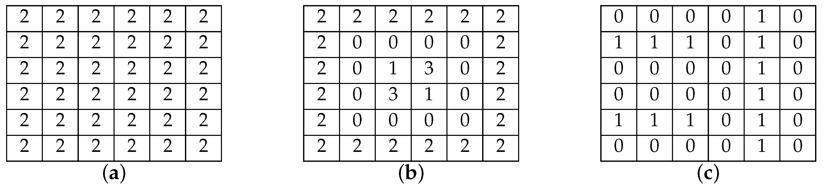
Firstly, the pattern must be represented as a rectangular (preferably square) array of symbols, where each symbol corresponds to one basic constituent of the pattern For example, in architecture, one element might correspond to a curved corner and another to a window. In our approach, we make use of only two symbols (1 or 0), which correspond to the presence or absence of a turbine in a particular small region in the layout. Examples of some small symbol arrays, two of which are from Klinger and Salingaros [18], are shown in Figure 4. Note that in the figure, the entries {0,1,2,3} denote symbols, and H denotes the harmony metric, which is defined next.
Once the symbol array is available, the harmony metric is computed by first of all evaluating a number of functions on the symbol array. Each function concerns one particular class of symmetry, either reflective, rotational or in relation to another pattern. The functions (nine of them) are listed in Table 1, and each function returns either one or zero depending on whether the pattern has the particular class of symmetry with which the function is concerned.
Before showing how the overall harmony of a pattern is computed, we must first define the value . This quantity, where is a pattern and B is a set of different patterns of the same size, is defined as follows:
The functions – measure top-level properties of the pattern. The functions – measure properties of the pattern in relation to all of the patterns in B. For these three latter functions, if matches any of the elements in B, then one is returned; otherwise (or if B is empty), zero is returned. Therefore, must return a value either between zero and nine if B is non-empty, or zero and six if B is empty.
We now define to be the set of all non-overlapping sub-patterns of that can be obtained by dividing into -sized subarrays. If the size of is , then will have four distinct elements, will have nine elements and will have one element. If the size of is , on the other hand, then .
The final harmony for a pattern can thus be defined as:
where , being an average across values computed by the h function, is also in the range of zero to nine inclusive. In the definition of H, the set N consists of positive integers, which are not greater than (and preferably divide evenly into) the smallest dimensionality of . The elements of N define the sizes of the sub-patterns to consider. In the original paper [18], , and we use the same values, although we do increase the sizes of the patterns being considered from to .
A brief consideration of Equation (11) should make clear the fact that what is being computed is the average of the harmonies of each sub-pattern at the various different scales defined by N. The inner summation computes the harmony for each particular scale.
Then, the average harmony across scales, represented by the outer summation and division by , is calculated. The resulting quantity is the final metric. Thus, a higher harmony indicates that the pattern contains more symmetries at the various scales, while a lower harmony indicates fewer multi-scale symmetries.
3. Optimising Wind Farm Layouts for Both Energy Efficiency and Harmony
This sections defines two new approaches that extend both TDA and the BlockCopy local search method with the harmony metric explained in the previous section. We name these new approaches TDA and BC.
The idea is fairly straightforward. Rather than optimising directly for energy efficiency (i.e., maximising F only, which is defined by Equation (9)), we instead replace F with a composite objective function obtained by adding F and H. This new objective function is:
Two key parts of the new approach are (i) a function that converts a layout (consisting of real-valued double coordinates) into a symbolic pattern array and (ii) a parameter that specifies how much influence harmony will have on the objective.
For the function, we simply divide the layout (which is square in our experiments) into “cells”. Each cell maps to a symbol in a symbol array representing the layout and corresponds to the number of turbines in that cell. As it turns out, on our test layouts, the cells were relatively small, and so, they only ever contain either one turbine or no turbines due to the minimum turbine distance constraint.
The choice of value for was a more difficult decision, however, and we therefore decided to test four different values: zero, corresponding to harmony having no influence on the optimisation process; 0.001 and 0.01, corresponding to harmony having small to medium effects on the objective function; and 0.1, corresponding to harmony being nearly equally weighted with energy efficiency. The choice of these values was made because the range of the H parameter () is nine-times the range of the F parameter (), and thus, small values of make sense. Larger values of would result in harmony overwhelming the combined objective function.
The case of is thus our baseline because it essentially reverts the TDA and BC approaches back into their original versions.
4. Experiments
To evaluate our new modified objective functions, we implemented Jensen’s far wake model and used it to simulate a wind farm layout of a size of 1.5 km ×1.5 km, with 64 turbines to be sited. The turbine power curve and the other settings for the wake model are described in Section 2.1. The optimisers used are the algorithms described previously. Each algorithm was initialised with a starting random layout created by iteratively adding turbines at random locations within the layout bounds, subject to the constraint of not placing any two turbines too closely together, until all 64 turbines were placed.
Samorani [21] describes three different problems of increasing complexity for testing wind farm layout optimization algorithms, and we adopted these three benchmark problems for our experiments. The problems, referred to as A, B and C, are described by Table 2.
Essentially, Problem A is the simplest benchmark, and comprises a single wind scenario in which wind blows with a single expected speed and in a single constant direction. The set of scenarios S therefore (used in Equation (9) for calculating F) consists of only a single element. Problem B, on the other hand, consists of 36 different wind scenarios, each differing only in the wind direction. Unlike Problem A, there is no dominant wind direction; instead, the expected wind speed is the same for all directions. Although this is an unrealistic setting, it is useful for testing purposes.
Problem C, on the other hand, is the the most interesting and challenging benchmark. In Problem C, as in Problem B, there are 36 possible wind directions. In Problem C’s case, however, for each different direction, there are also three different expected wind speeds. Furthermore, there is a clear dominant wind direction: the probability of the greatest wind speed (and therefore, the greatest power production) is maximised at . In total, this problem comprises 108 different wind scenarios.
Since Samorani [21] only describes this problem benchmark graphically by means of a histogram of wind speeds vs. directions, in order to implement this benchmark, we reverse-engineered the probabilities from his published chart. The probabilities we used for Problem C are given in Table 3.
To summarise, our experiments consist of algorithms with a new modified objective function (TDA and BC) with four different values on three different benchmark problems. This amounts to 24 different configurations.
Next, for each configuration, we ran 30 repetitions. Each repetition consisted of one run of a local search algorithm for 20,000 iterations. We note that the number of iterations is significantly higher than the number of iterations (2000) in a previous comparison of TDA and BlockCopy [12].
5. Results
The summary results are depicted in Figure 5, Figure 6 and Figure 7. The figures show the mean and maximum F and H values achieved by algorithm over all thirty runs. We note in this section that our use of the term “performance” refers to the best objective values achieved by the various algorithms and not, as is the common interpretation, to computational efficiency.
Broadly speaking the figures show that BlockCopy local search “outperforms” TDA in terms of energy efficiency when is small. The difference between the algorithms for Problem A is up to approximately 10%; for Problems B and C, the difference is less pronounced.
In terms of the harmony metric, however, the BlockCopy approach generally scores a much higher value than TDA, especially as increases. This is most likely due to the approximate preservation of translational symmetry, a property of the BlockCopy operator discussed earlier.
Overall, under both algorithms, the best layouts degrade in terms of energy efficiency as increases. This energy loss is approximately 6% on average for Problem C. Analysing the final best layouts produced by every 30-run configuration, we found that there is a significant negative correlation between final F and H values. This confirms that the two objectives, energy efficiency and harmony, tend to trade off. Testing more advanced multi-objective algorithms may be worthwhile in the future.
Next, we were also interested in the statistically-significant differences in performances for a more quantitative comparison.
To this end, we performed a post-hoc Tukey honestly significant difference test comparing the F value mean between all eight techniques on each of the three different benchmark problems. The test was performed at 95% significance. The results indicate that for Problems A and B, there is no significant difference in mean performance between algorithms in the following sets:
- {(TDA, ), (TDA, ), (TDA, )}
- {(BC, ), (BC, ), (BC, )}
- {(TD, ), (BC, )} (Problem B only)
The result of these tests show that small to moderate values for do not significantly impact on optimisation performance. The figures quantify the actual difference in mean performances between algorithms.
For Problem C, the situation is slightly more complex. The sets of algorithms with no statistically-significant difference in mean performance are:
- {(BC, ), (BC, ), (TDA, )}
- {(TDA, ), (TDA, ), (BC, )}
- {(TDA, ), (BC, ), (TDA, )}
- {(TDA, )}
- {(BC, )}
These results clearly are more difficult to interpret, which suggests that no conclusion can be drawn without more repetitions of the algorithms.
We note at this point that tests for statistical significance only determine the likelihood of average algorithm performance variations. The results, however, show that best-of-run performance is often quite different from the mean. This is illustrated most clearly in Figure 7a for the algorithm BC with : the best layout identified by the algorithm is comparable to average layouts found by the other algorithms with , even though the mean F value performance of this algorithm is quite low.
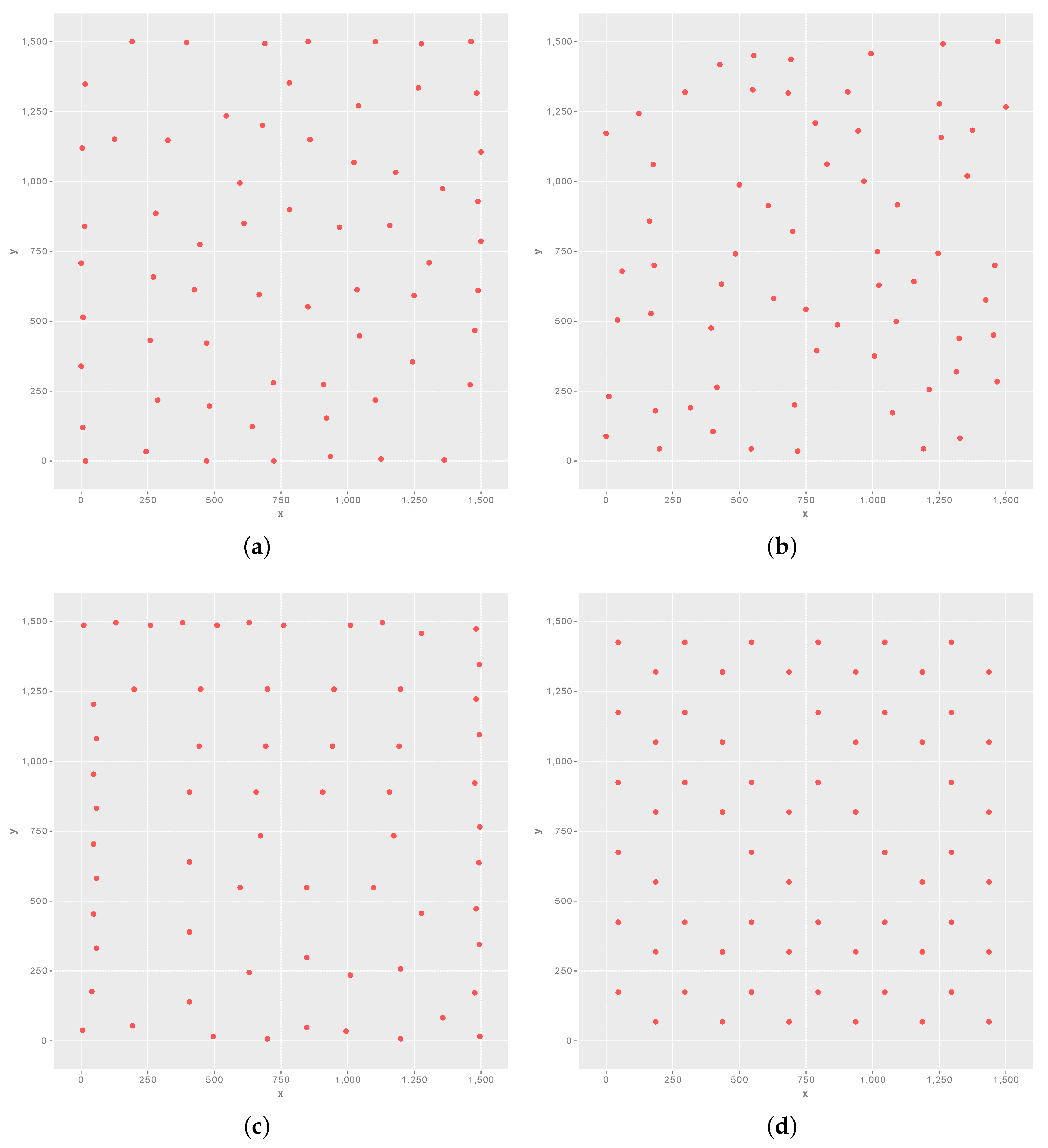
Finally, we examined visually some of the optimal layouts found after different runs of the various techniques. Examples of different optimised layouts are shown in Figure 8, Figure 9 and Figure 10.
Focussing firstly on Figure 8, which depicts some layout solutions to Problem A, we can see clearly the difference between the TDA and BC. For the TDA-based layouts (Figure 8a,b), the arrangement of turbines has a clear random character. This is even the case where the value is at its highest in Figure 8b; in this case, the H objective is not much different than it is in (a), where it is not optimised at all.
In contrast, the BC algorithms tend to produce more patterned layouts. For example, Figure 8c does not make use of the harmony metric at all, but it still produces a degree of translational symmetry across the layout. When is high however, as in Figure 8d, the translational symmetry is increased dramatically to produce a considerably more regular arrangement of turbines.
A somewhat different story can be told for the examples shown in Figure 9, which depicts example solutions to Problem B. This benchmark problem has no dominant wind direction, which becomes evident when the layouts are examined. To illustrate, both algorithms optimising solely for efficiency (see Figure 9a,c) tend to push turbines out to the furtherest possible edge of the layouts, thus maximising the space between turbines in all directions. The BC algorithm interestingly produces a layout that is somewhat grid-like in structure in this case (see Figure 9c).
Finally, Figure 10 depicts selected solutions to Problem C. Similar trends can be observed in the solutions to this problem as were observed for the other problems. For example, BC produces more regular layouts than TDA regardless of the value on this problem. Also of considerable interest with regards to this problem is the difference in efficiencies achieved: the BC algorithm with produces an optimal layout in the figure with an efficiency of only about half a percent less than TDA’s best layout with .
As a final comment, it will be pointed out that the harmony metric is maximised for patterns that are completely uniform. For example, see Figure 4a. The practical effect of this bias is that the search is more likely to be focussed on sparse layouts; i.e., layouts with several empty blocks. This is because empty blocks correspond to uniform patterns, which maximise H.
To illustrate, see Figure 8d for an extreme example, and Figure 10d for a less extreme example. The practical consequences of this are considerable, since less land can be used for the same or approximately the same efficiency. This may positively impact on both the cost of land (e.g., see Chen and McDonald [27]) and the effect on wildlife (e.g., see the survey on environmental implications of wind energy by Tabassum-Abbasi et al. [6]). This finding also suggests that purely regular approaches (e.g., Neubert et al.’s [14]) may not be ideal solutions to this problem because such approaches distribute turbines uniformly across the layout without any chance of free space areas appearing.
6. Conclusions
To conclude, we have investigated a metaheuristic biobjective optimisation approach to solving the wind farm layout optimisation problem, in which one objective concerns maximising layout aesthetics while the other concerns maximising energy efficiency. The aesthetics of layouts is an important consideration that most other literature in this field to date has not considered. Our experiments reported here were successful and encourage future research to further refine this initial approach. In particular, while the Jensen model is adequate for this initial work, future work should explore more realistic wind farm simulations that better account for both wind (e.g., [28]) and partial wakes (e.g., [29]).
As mentioned in the Introduction, there are two main limitations of the work presented here. Firstly, our approach is largely constrained to two-dimensional layouts, as would typically be encountered offshore or on sites that are plains. Clearly, therefore, Salingaros’ approach must be generalised to three dimensions before the same ideas can be applied to other types of site. Our current thinking is that there are two possible approaches to this generalisation: (i) topography could be included in the definition of the symbols, which would complicate the definition of what a symbol is somewhat (e.g., a turbine on the top of a knoll would result in a different symbol compared to a turbine at the same relative position, but in the middle of plain); or alternatively (ii) the method could be generalised to include transformations in the z dimension; this approach would require expanding the set of symmetries listed in Table 1 to include all 3D symmetries, as well.
The second main limitation of this work is that it focusses on the overhead view of the layout only and assumes by default that aesthetics is uniformly important across the entire layout. This is in fact not correct for farms located near places that people frequent, such as nearby towns, tourist attractions and highways. In such situations, the aesthetics of the portion of the farm in clear view of the people will be far more important than the parts of the farm that are obscured. Therefore, the vantage point is important. Our “global” approach to aesthetics could therefore be complemented by a corresponding “local” approach that takes into account viewpoint. The local approach could take an image aesthetics-based approach and render the farm and its surrounding terrain, skyline and other features as an eye-level scene, and then assess its aesthetics using machine learning. Marchesotti et al. [30] is one example of such an approach that could be gainfully employed here.
Acknowledgments
The authors thank the University of Waikato, Hamilton, New Zealand, for supporting this research.
Author Contributions
Michael Mayo conceived and designed the experiments; Michael Mayo and Maisa Daoud performed the experiments; Michael Mayo analyzed the data; Michael Mayo wrote the paper.
Conflicts of Interest
The authors declare no conflict of interest.
References
- Global Wind Energy Council. Global Wind Energy Outlook 2014; Global Wind Energy Council: Brussels, Belgium, 2014. [Google Scholar]
- London Array Brochure. Online PDF Brochure. Available online: http://www.londonarray.com/wp-content/uploads/London-Array-Brochure.pdf (accessed on 9 November 2015).
- Watts, J. Winds of Change Blow through China as Spending on Renewable Energy Soars. The Guardian. 2012. Available online: http://www.theguardian.com/world/2012/mar/19/china-windfarms-renewable-energy (accessed on 23 March 2017).
- Dai, K.; Bergot, A.; Liang, C.; Xiang, W.N.; Huang, Z. Environmental issues associated with wind energy—A review. Renew. Energy 2015, 75, 911–921. [Google Scholar] [CrossRef]
- Piorkowski, M.D.; Farnsworth, A.J.; Fry, M.; Rohrbaugh, R.W.; Fitzpatrick, J.W.; Rosenberg, K.V. Research priorities for wind energy and migratory wildlife. J. Wildl. Manag. 2012, 76, 451–456. [Google Scholar] [CrossRef]
- Tabassum-Abbasi; Premalatha, M.; Abbasi, T.; Abbasi, S. Wind energy: Increasing deployment, rising environmental concerns. Renew. Sustain. Energy Rev. 2014, 31, 270–288. [Google Scholar]
- Tsoutsos, T.; Gouskos, Z.; Karterakis, S.; Peroulaki, E. Aesthetic Impact from Wind Parks; Technical Report; Technical University of Crete: Chania, Greece, 2006. [Google Scholar]
- Mosetti, G.; Poloni, C.; Diviacco, B. Optimization of wind turbine positioning in large wind farms by means of a genetic algorithm. J. Wind Eng. Ind. Aerodyn. 1994, 51, 105–116. [Google Scholar] [CrossRef]
- Wagner, M.; Day, J.; Neumann, F. A fast and effective local search algorithm for optimizing the placement of wind turbines. Renew. Energy 2013, 51, 64–70. [Google Scholar] [CrossRef]
- Rodrigues, S.M.F.; Bauer, P.; Pierik, J. Modular Approach for the Optimal Wind Turbine Micro Siting Problem Through CMA-ES Algorithm. In Proceedings of the 15th Annual Conference Companion on Genetic and Evolutionary Computation, Amsterdam, The Netherlands, 6–10 July 2013; pp. 1561–1568. [Google Scholar]
- Guirguis, D.; Romero, D.A.; Amon, C.H. Toward efficient optimization of wind farm layouts: Utilizing exact gradient information. Appl. Energy 2016, 179, 110–123. [Google Scholar] [CrossRef]
- Mayo, M.; Zhen, C. BlockCopy-based operators for evolving efficient wind farm layouts. In Proceedings of the 2016 IEEE Congress on Evolutionary Computation, Vancouver, BC, Canada, 24–29 July 2016; pp. 1085–1092. [Google Scholar]
- Mayo, M.; Daoud, M. Informed mutation of wind farm layouts to maximise energy harvest. Renew. Energy 2016, 89, 437–448. [Google Scholar] [CrossRef]
- Neubert, A.; Shah, A.; Schlez, W. Maximum Yield from Symmetrical Wind Farm Layouts. In Proceedings of the 10th German Wind Energy Conference, DEWEK, Bremen, Germany, 17–18 November 2010. [Google Scholar]
- Al-Yahyai, S.; Charabi, Y.; Gastli, A. Geometrical approach for wind farm symmetrical layout design optimization. In Proceedings of the 2015 IEEE 8th GCC Conference and Exhibition (GCCCE), Muscat, Oman, 1–4 February 2015; pp. 1–6. [Google Scholar]
- Mayo, M.; Daoud, M.; Zheng, C. Randomising block sizes for BlockCopy-based wind farm layout optimisation. In Proceedings of the 20th Asia Pacific Symposium on Intelligent and Evolutionary Systems, Canberra, Australia, 16–18 November 2016; pp. 277–289. [Google Scholar]
- Salingaros, N. Life and complexity in architecture from a thermodynamic analogy. Phys. Essays 1997, 10. [Google Scholar] [CrossRef]
- Klinger, A.; Salingaros, N. A pattern measure. Environ. Plan. B Plan. Des. 2000, 27, 537–547. [Google Scholar] [CrossRef]
- Jensen, N. A Note on Wind Generator Interaction; Technical Report; Risø DTU National Laboratory for Sustainable Energy: Roskilde, Denmark, 1983. [Google Scholar]
- Katic, I.; Høstrup, J.; Jensen, N. A simple model for cluster efficiency. In Proceedings of the Europe and Wind Energy Association Conference and Exhibition, Rome, Italy, 7–9 October 1986. [Google Scholar]
- Samorani, M. The Wind Farm Layout Optimization Problem. In Handbook of Wind Power Systems; Pardolas, P., Ed.; Springer: Berlin/Heidelberg, Germany, 2013; pp. 21–38. [Google Scholar]
- Shakoor, R.; Hassan, M.; Raheem, A.; Wu, Y. Wake effect modelling: A review of wind farm layout optimization using Jensen’s model. Renew. Sustain. Energy Rev. 2016, 58, 1048–1059. [Google Scholar] [CrossRef]
- Song, Z.; Zhang, Z.; Chen, X. The decision model of 3-dimensional wind farm layout design. Renew. Energy 2016, 85, 248–258. [Google Scholar] [CrossRef]
- Wilson, D.; Cussat-Blanc, S.; Veeramachaneni, K.; O’Reilly, U.; Luga, H. A Continuous Development Model for Wind Farm Layout Optimization. In Proceedings of the 2014 Conference on Genetic and Evolutionary Computation, Vancouver, BC, Canada, 12–16 July 2014; pp. 745–752. [Google Scholar]
- Den Heijer, E.; Eiben, A. Comparing Aesthetic Measures for Evolutionary Art. In Applications of Evolutionary Computation; Lecture Notes in Computer Science; Springer: Berlin/Heidelberg, Germany, 2010; Volume 6025, pp. 311–320. [Google Scholar]
- Galanter, P. Computational Aesthetic Evaluation: Past and Future. In Computers and Creativity; McCormack, J., d’Inverno, M., Eds.; Springer: Berlin/Heidelberg, Germany, 2012; Chapter 11; pp. 255–293. [Google Scholar]
- Chen, L.; MacDonald, E. Considering Landowner Participation in Wind Farm Layout Optimization. J. Mech. Des. 2012, 134, 084506. [Google Scholar] [CrossRef]
- Feng, J.; Shen, W. Modelling wind for wind farm layout optimisation using joint distribution of wind speed and wind direction. Energies 2015, 8, 3075–3092. [Google Scholar] [CrossRef]
- Feng, J.; Shen, W.Z. Solving the wind farm layout optimization problem using random search algorithm. Renew. Energy 2015, 78, 182–192. [Google Scholar] [CrossRef]
- Marchesotti, L.; Murray, N.; Perronnin, F. Discovering beautiful image attributes for aesthetic image analysis. Int. J. Comput. Vis. 2015, 113, 246–266. [Google Scholar] [CrossRef]
Figure 1.
Depiction of the wake effect (reproduced from [21]).
Figure 1.
Depiction of the wake effect (reproduced from [21]).
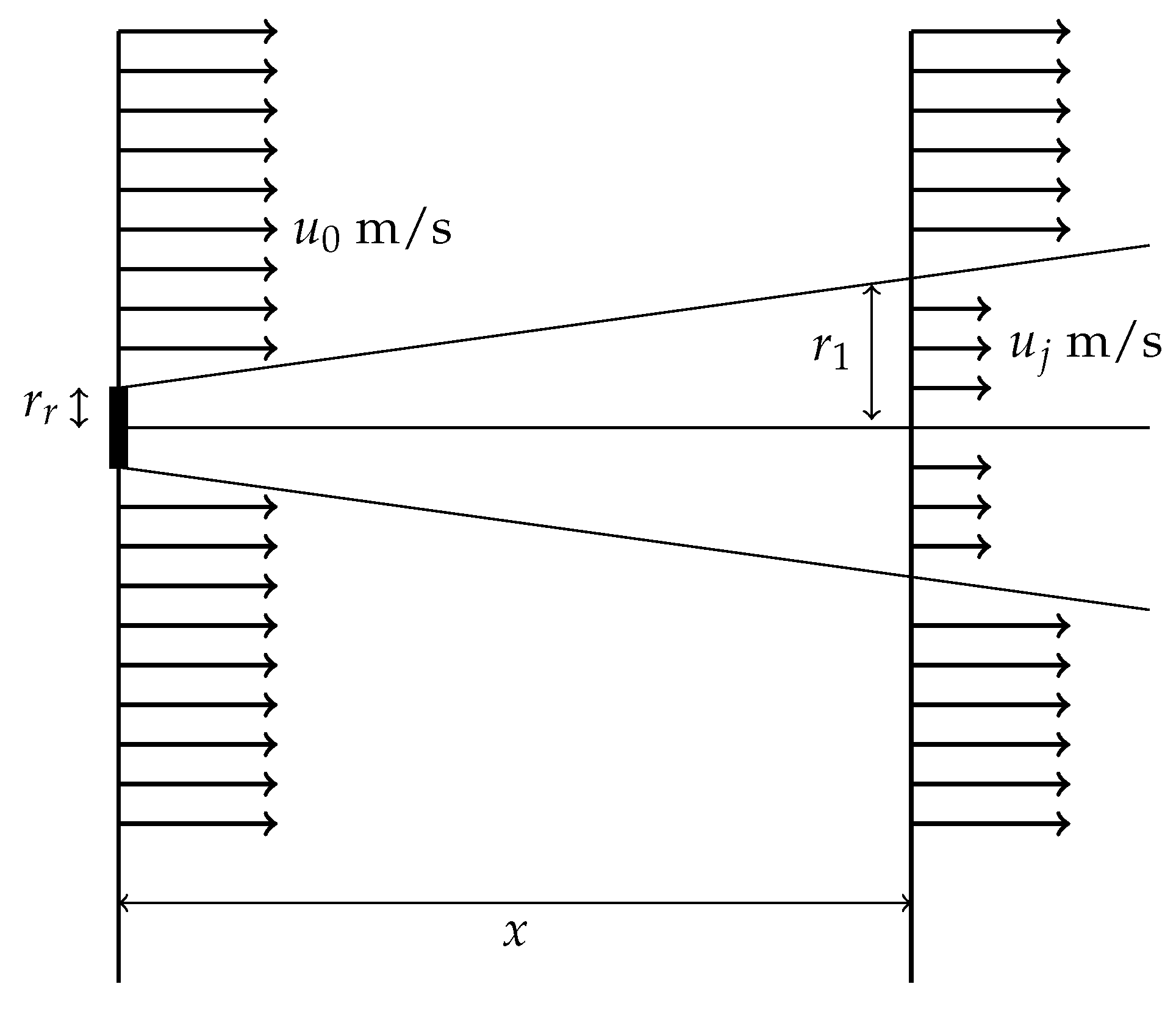
Figure 2.
Illustration of the Turbine Displacement Algorithm (TDA) operator. In this example, and the displacement vector for (and its potential inverted displacement vector after rescaling to prevent collisions) are shown.
Figure 2.
Illustration of the Turbine Displacement Algorithm (TDA) operator. In this example, and the displacement vector for (and its potential inverted displacement vector after rescaling to prevent collisions) are shown.

Figure 3.
Illustration of the BlockCopy operator. In this example, the left block of a small layout is duplicated to the right-hand side of the layout. (a) Initial layout with selected source block; (b) final layout showing new target block.
Figure 3.
Illustration of the BlockCopy operator. In this example, the left block of a small layout is duplicated to the right-hand side of the layout. (a) Initial layout with selected source block; (b) final layout showing new target block.

Figure 4.
Examples of three patterns and their harmonies, computed using levels . (a) ; (b) ; (c) .

Figure 5.
Optimisation performance over 30 runs with different values on Problem A. Figures show final best (a) F values and (b) H values.
Figure 5.
Optimisation performance over 30 runs with different values on Problem A. Figures show final best (a) F values and (b) H values.
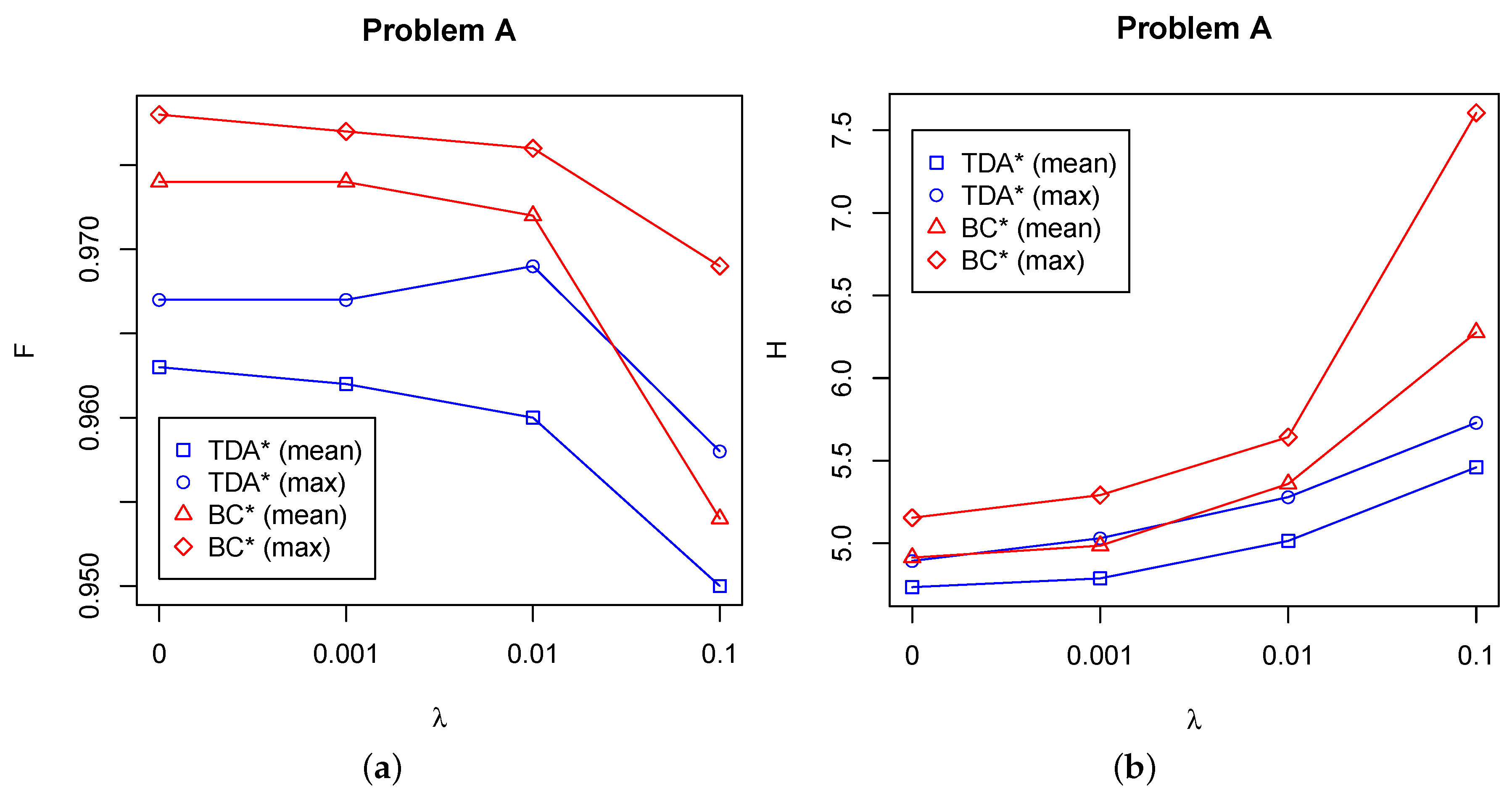
Figure 6.
Optimisation performance over 30 runs with different values on Problem B. Figures show final best (a) F values and (b) H values.
Figure 6.
Optimisation performance over 30 runs with different values on Problem B. Figures show final best (a) F values and (b) H values.
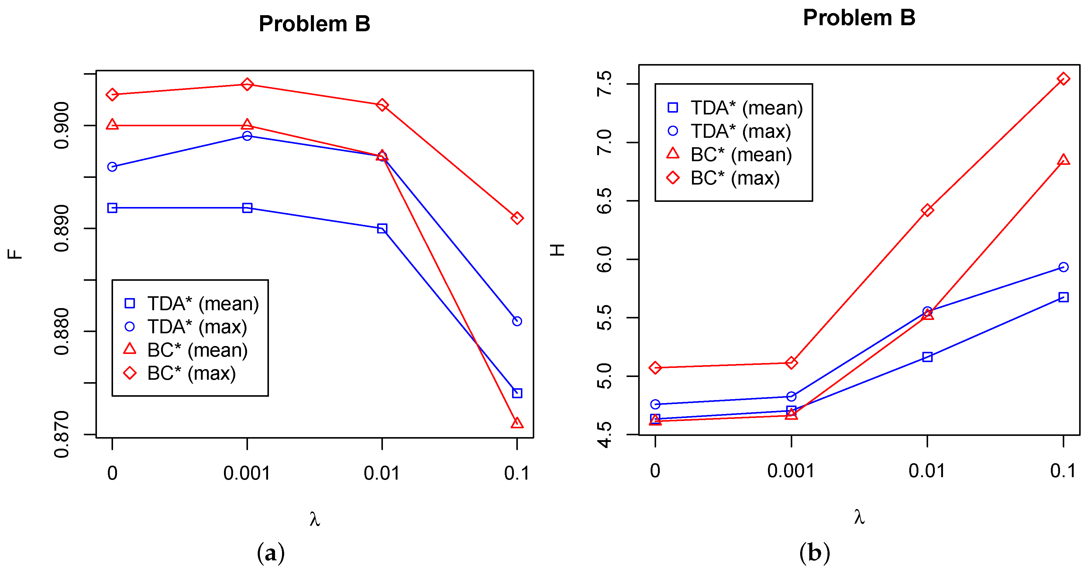
Figure 7.
Optimisation performance over 30 runs with different values on Problem C. Figures show final best (a) F values and (b) H values.
Figure 7.
Optimisation performance over 30 runs with different values on Problem C. Figures show final best (a) F values and (b) H values.
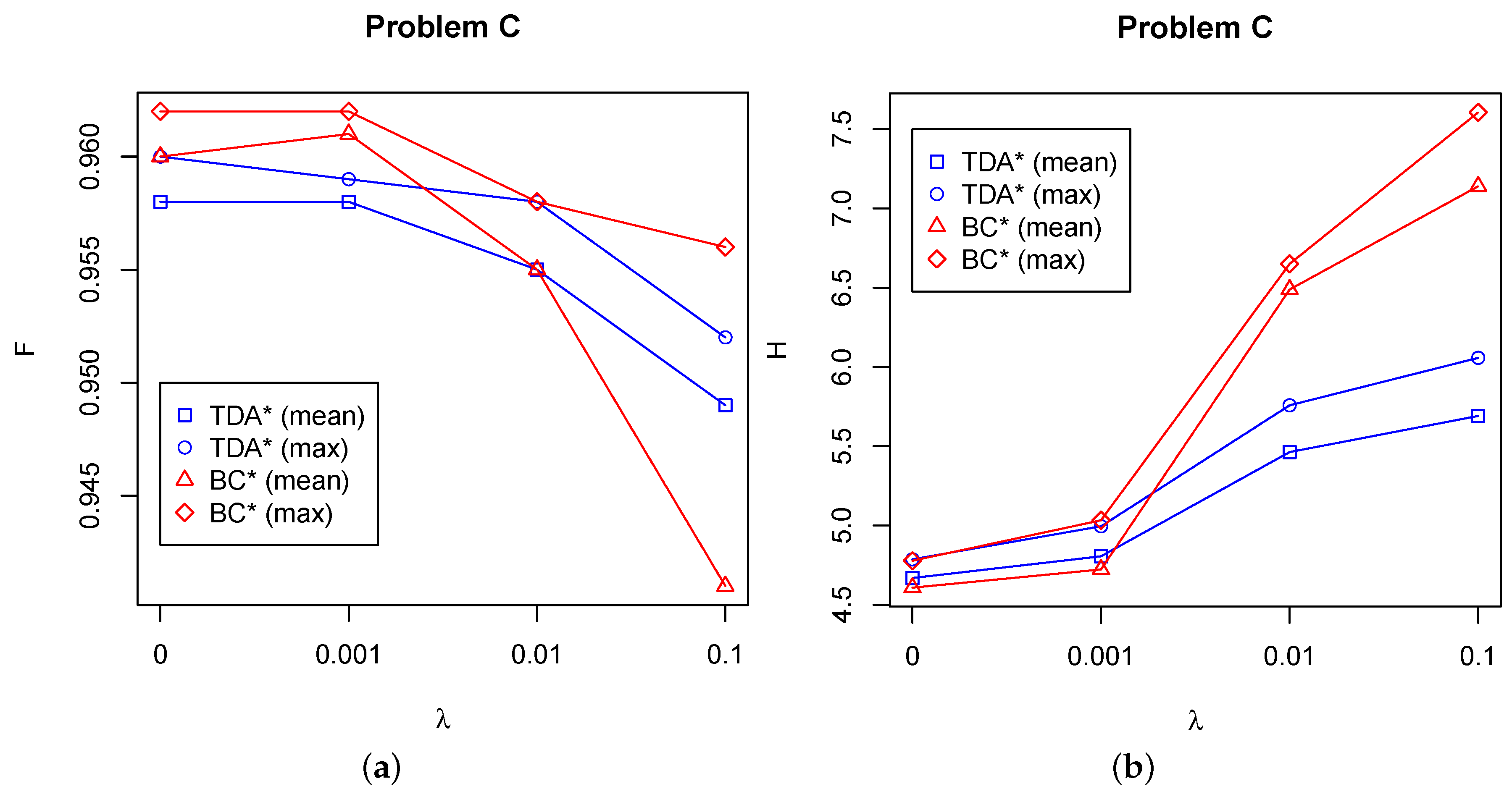
Figure 8.
Example layouts produced by the modified Turbine Displacement Algorithm (TDA) (a,b) and the modified BlockCopy algorithm (BC) (c,d) on Problem A. (a) TDA, , F = 0.967, ; (b) TDA, ; (c) BC, ; (d) BC, .
Figure 8.
Example layouts produced by the modified Turbine Displacement Algorithm (TDA) (a,b) and the modified BlockCopy algorithm (BC) (c,d) on Problem A. (a) TDA, , F = 0.967, ; (b) TDA, ; (c) BC, ; (d) BC, .
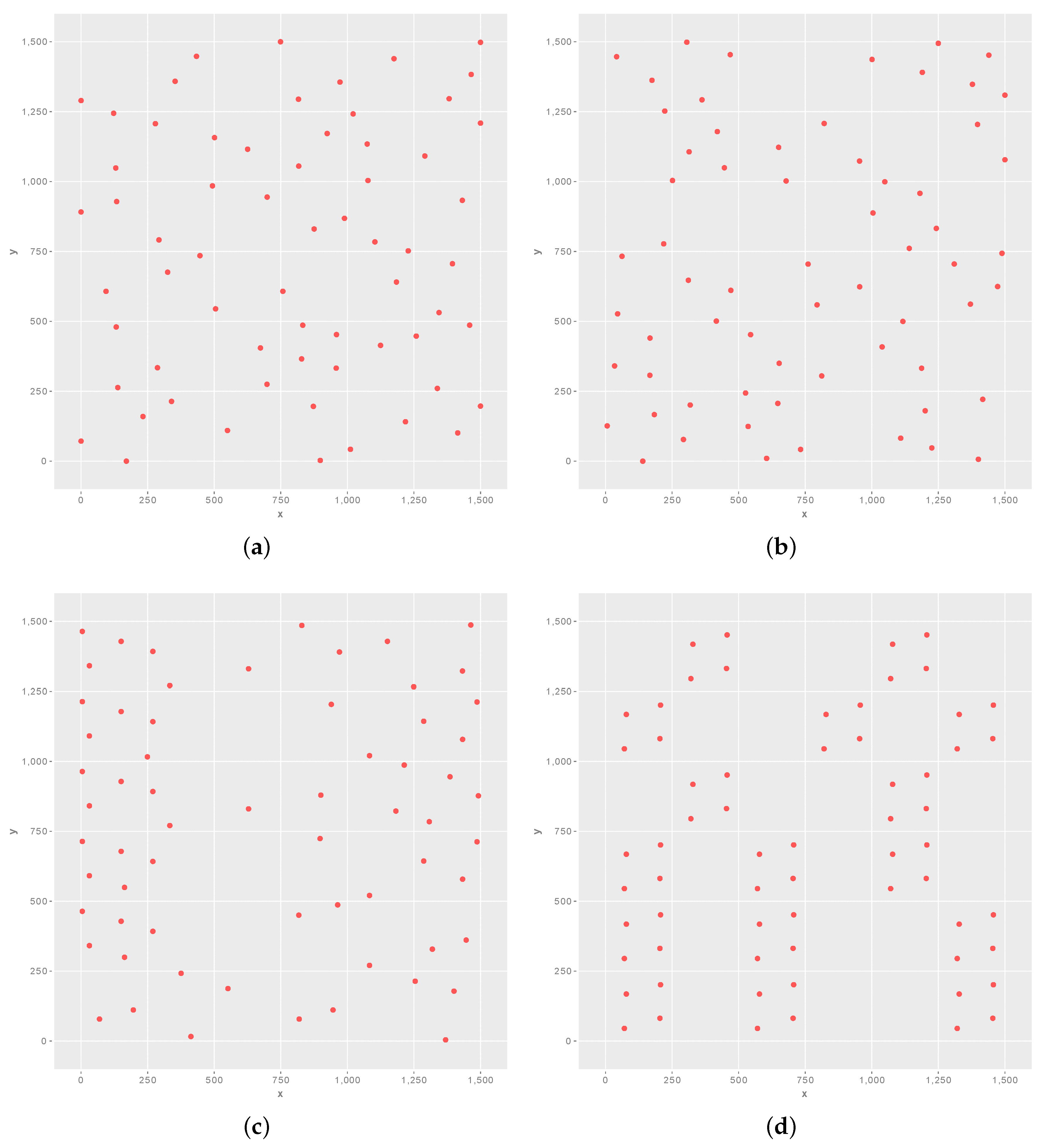
Figure 9.
Example layouts produced by the modified Turbine Displacement Algorithm (TDA) (a,b) and the modified BlockCopy algorithm (BC) (c,d) on Problem B. (a) TDA, , , ; (b) TDA, ; (c) BC, ; (d) BC, .
Figure 9.
Example layouts produced by the modified Turbine Displacement Algorithm (TDA) (a,b) and the modified BlockCopy algorithm (BC) (c,d) on Problem B. (a) TDA, , , ; (b) TDA, ; (c) BC, ; (d) BC, .
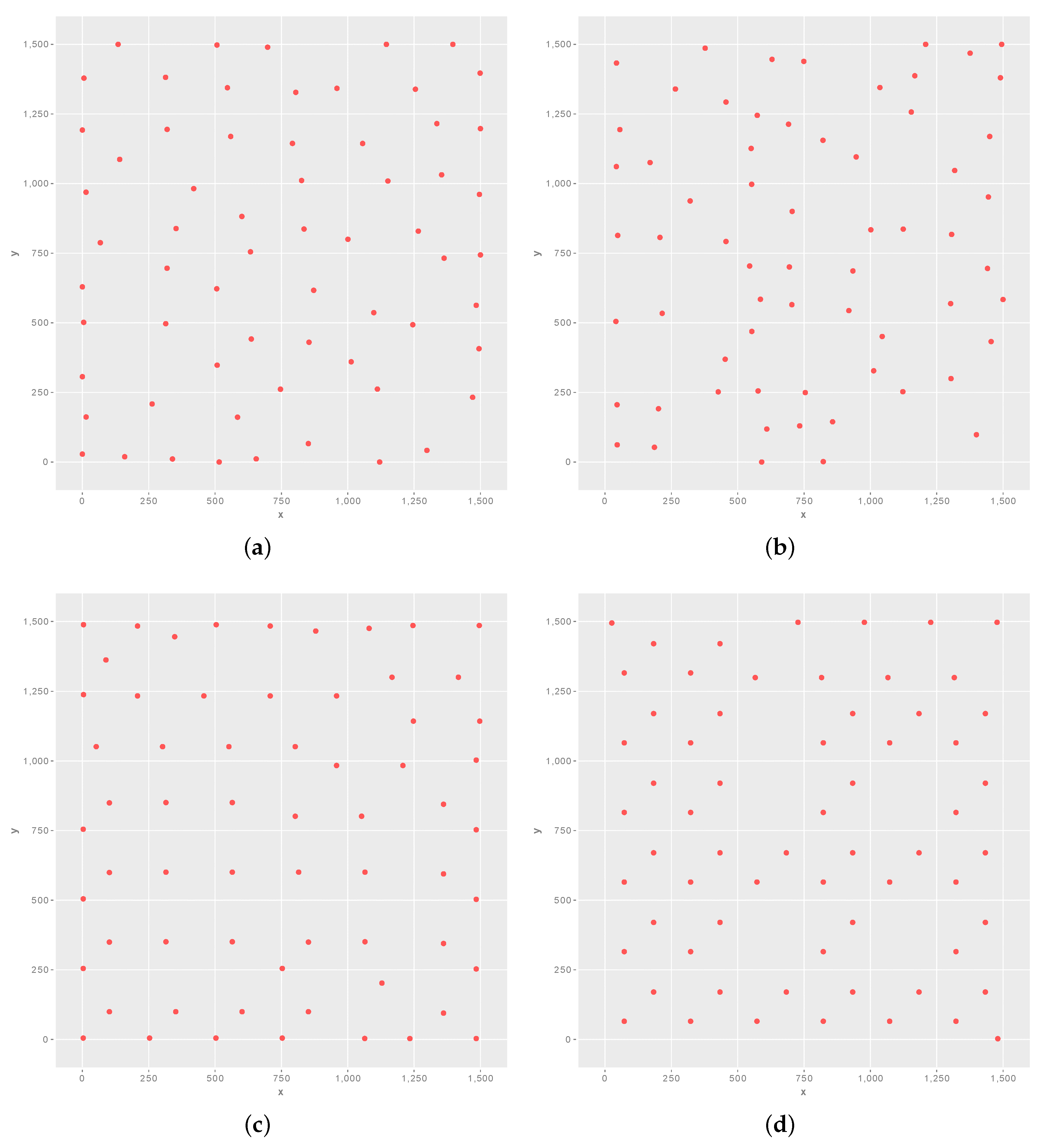
Figure 10.
Example layouts produced by the modified Turbine Displacement Algorithm (TDA) (a,b) and the modified BlockCopy algorithm (BC) (c,d) on Problem C. (a) TDA, , ; (b) TDA, ; (c) BC, ; (d) BC, , .
Figure 10.
Example layouts produced by the modified Turbine Displacement Algorithm (TDA) (a,b) and the modified BlockCopy algorithm (BC) (c,d) on Problem C. (a) TDA, , ; (b) TDA, ; (c) BC, ; (d) BC, , .


Table 1.
The six possible internal symmetries and the three additional hierarchical symmetries required to compute the harmony metric. Each h value is either one or zero.
Table 1.
The six possible internal symmetries and the three additional hierarchical symmetries required to compute the harmony metric. Each h value is either one or zero.
| Harmony | Description |
|---|---|
| Symmetry about the x axis. | |
| Symmetry about the y axis. | |
| Symmetry about the diagonal. | |
| Symmetry about the diagonal. | |
| rotational symmetry. | |
| rotational symmetry. | |
| Translational symmetry with another pattern. | |
| Translation plus reflectional symmetry with another pattern. | |
| Translation plus rotational ( or ) symmetry with another pattern. |
Table 2.
Problems from Samorani [21].
Table 2.
Problems from Samorani [21].
| Problem | Direction(s) | Expected Speed(s) | #Wind Scenarios |
|---|---|---|---|
| A | {} | {12 m/s} | 1 |
| B | {} | {12 m/s} | 36 |
| C | {} | {8 m/s, 12 m/s, 17 m/s} | 108 |
Table 3.
Probabilities used for the 108 wind scenarios under Problem C (rounded to three significant figures) derived from a chart in [21]. Please note that the first row the table, labelled “0∘ to 260∘”, represents 27 rows, each of which have the same values. We have written these values once only to prevent unnecessary duplication in the table.
| Direction | m/s | m/s | m/s |
|---|---|---|---|
| 0∘ to 260∘ | 0.00404 | 0.00865 | 0.0115 |
| 270∘ | 0.00404 | 0.0107 | 0.0127 |
| 280∘ | 0.00404 | 0.0121 | 0.0156 |
| 290∘ | 0.00404 | 0.0141 | 0.0185 |
| 300∘ | 0.00404 | 0.0138 | 0.0300 |
| 310∘ | 0.00404 | 0.0190 | 0.0352 |
| 320∘ | 0.00404 | 0.0138 | 0.0300 |
| 330∘ | 0.00404 | 0.0141 | 0.0185 |
| 340∘ | 0.00404 | 0.0121 | 0.0156 |
| 350∘ | 0.00404 | 0.0107 | 0.0127 |
© 2017 by the authors. Licensee MDPI, Basel, Switzerland. This article is an open access article distributed under the terms and conditions of the Creative Commons Attribution (CC BY) license (http://creativecommons.org/licenses/by/4.0/).
Share and Cite
MDPI and ACS Style
Mayo, M.; Daoud, M. Aesthetic Local Search of Wind Farm Layouts. Information 2017, 8, 39. https://doi.org/10.3390/info8020039
AMA Style
Mayo M, Daoud M. Aesthetic Local Search of Wind Farm Layouts. Information. 2017; 8(2):39. https://doi.org/10.3390/info8020039
Chicago/Turabian StyleMayo, Michael, and Maisa Daoud. 2017. "Aesthetic Local Search of Wind Farm Layouts" Information 8, no. 2: 39. https://doi.org/10.3390/info8020039
Note that from the first issue of 2016, this journal uses article numbers instead of page numbers. See further details here.