
Optimal Threshold Determination for Discriminating Driving Anger Intensity Based on EEG Wavelet Features and ROC Curve Analysis


Abstract
:1. Introduction
2. Materials and Method
2.1. Participants
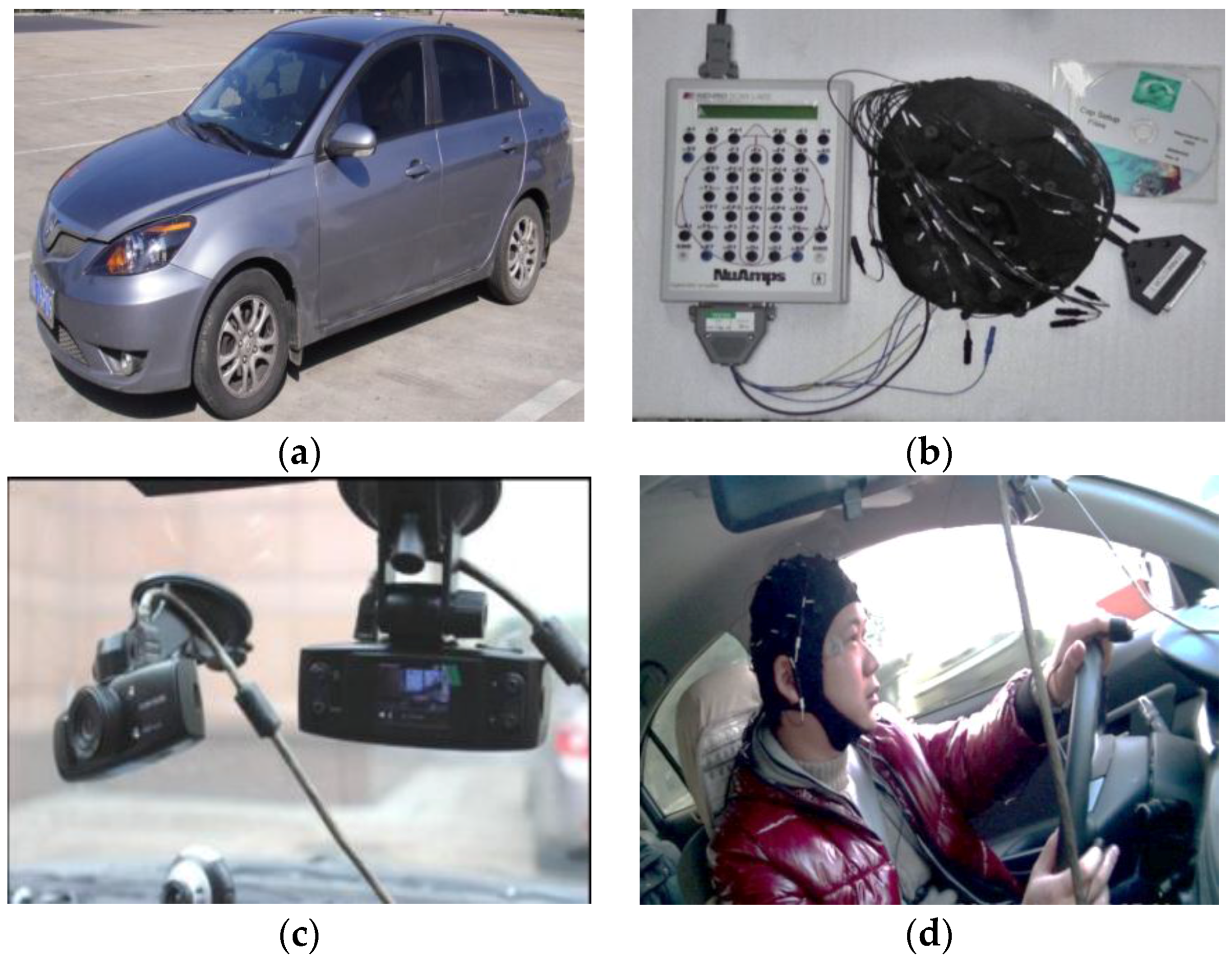
2.2. Apparatus
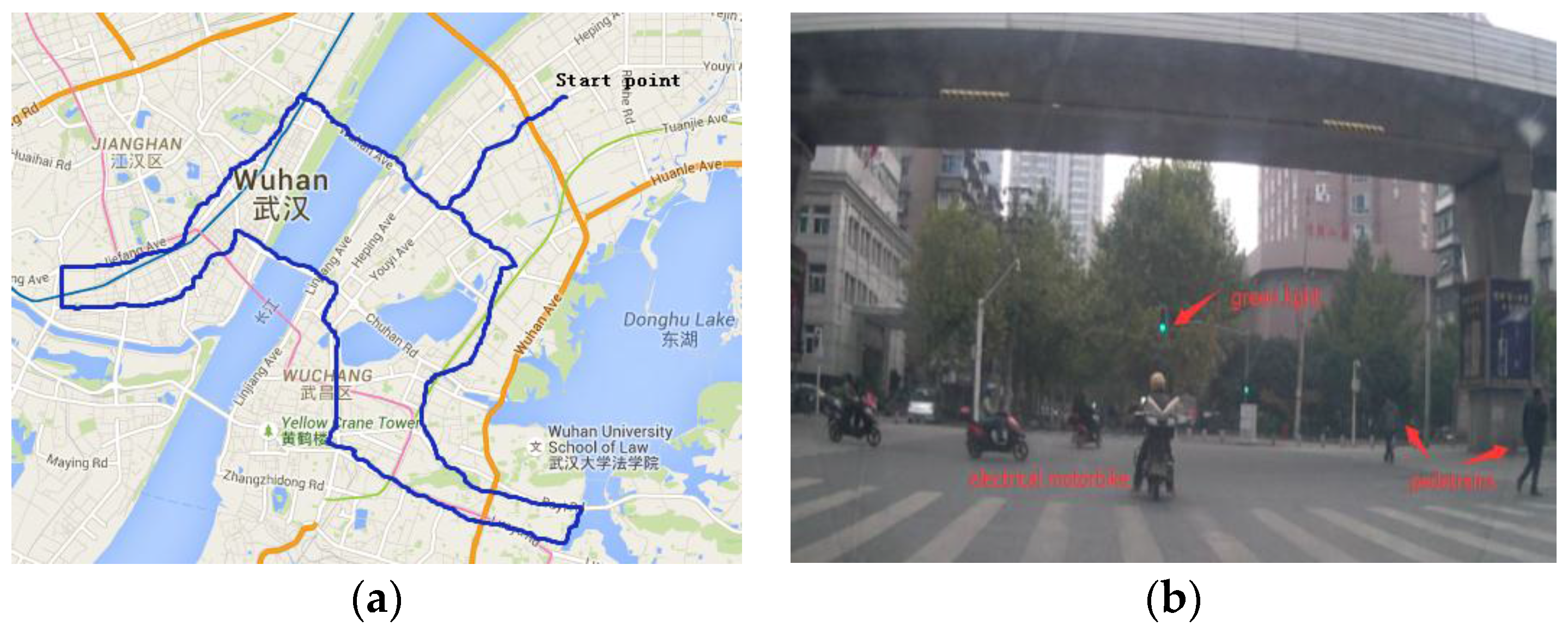
2.3. Driving Scenario Design
2.4. Experiment Procedure
3. EEG Features Extraction
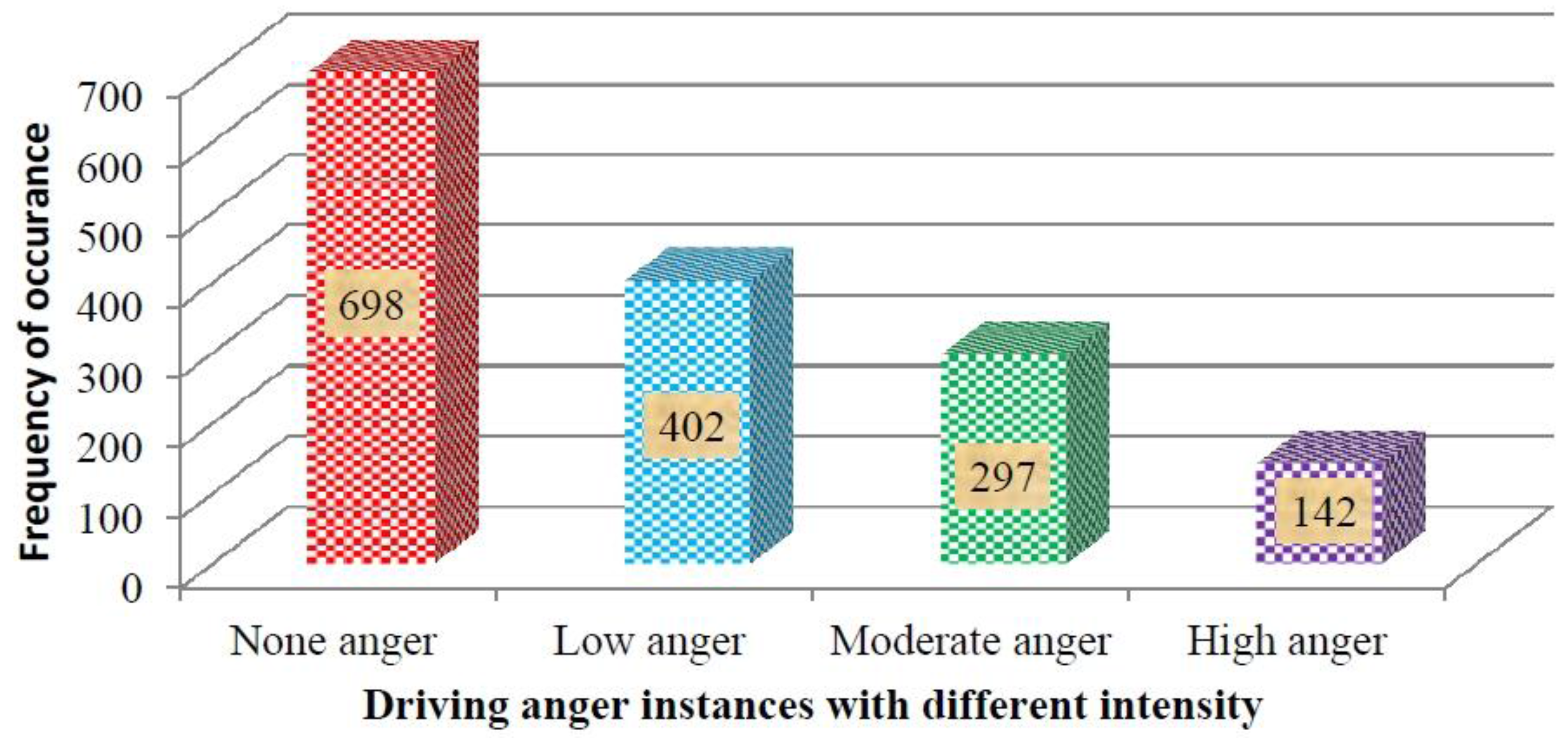
3.1. Anger Intensity Labeling
3.2. Signal Preprocessing of EEG
3.3. Artifact Removal Based on Discrete Wavelet Transform
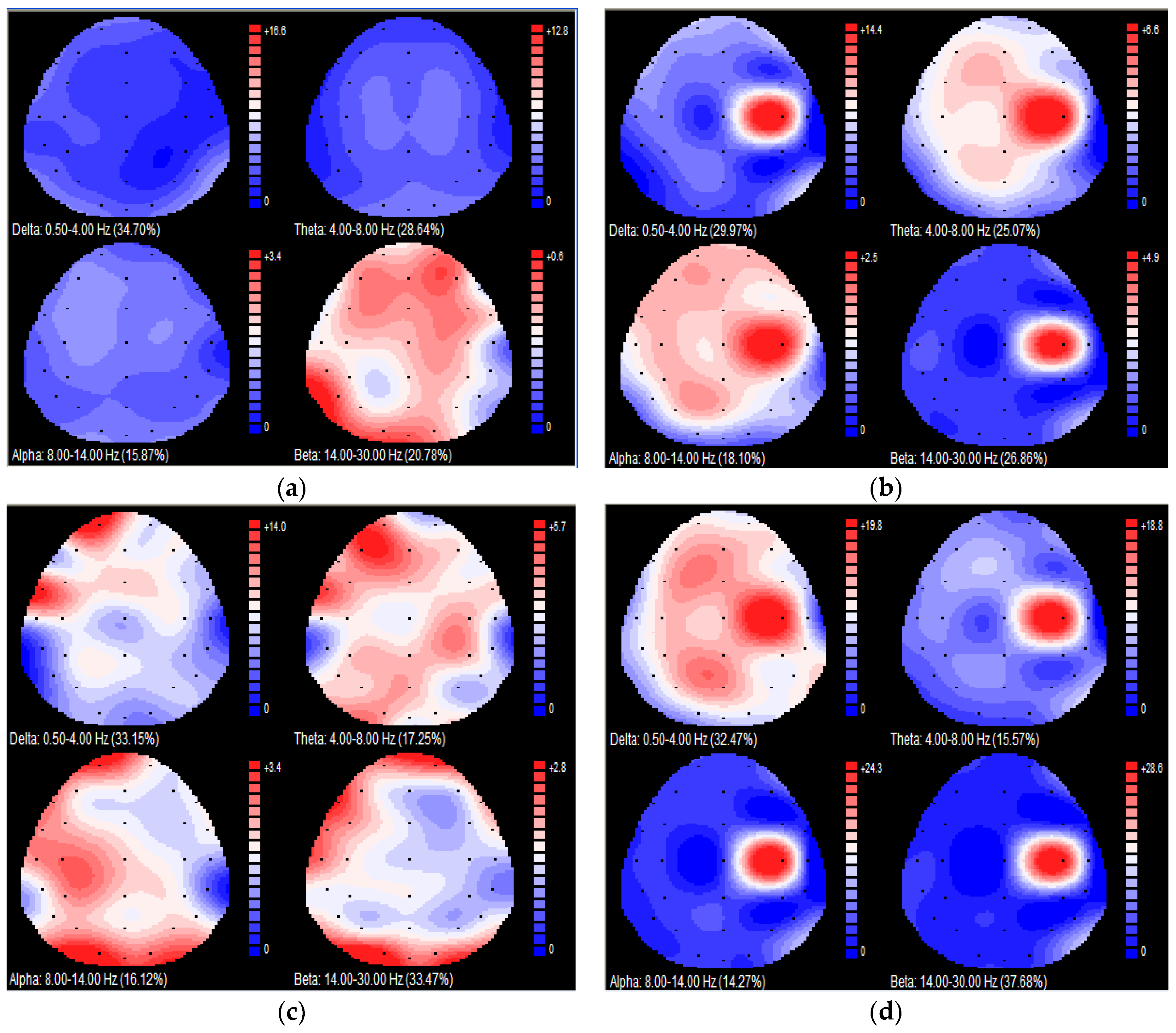
3.4. Extraction of Relative Wavelet Energy
3.5. Feature Selection for Discriminating Different Driving Anger States
4. Determining Optimal Threshold for Different Driving Anger Intensity
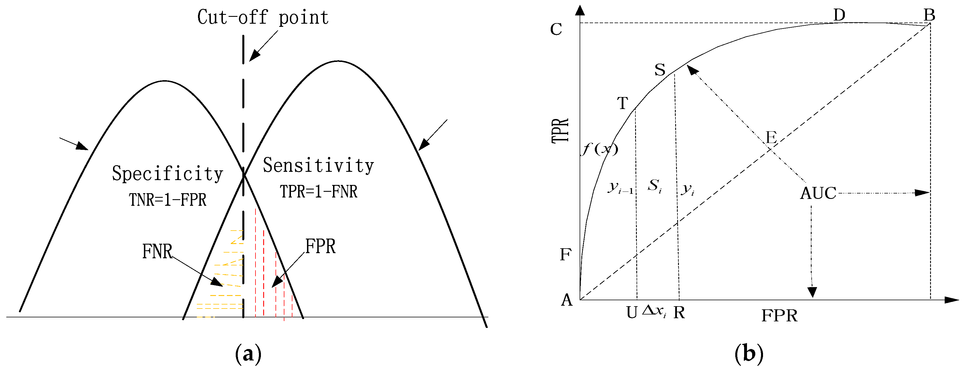
4.1. Method of ROC Curve Analysis
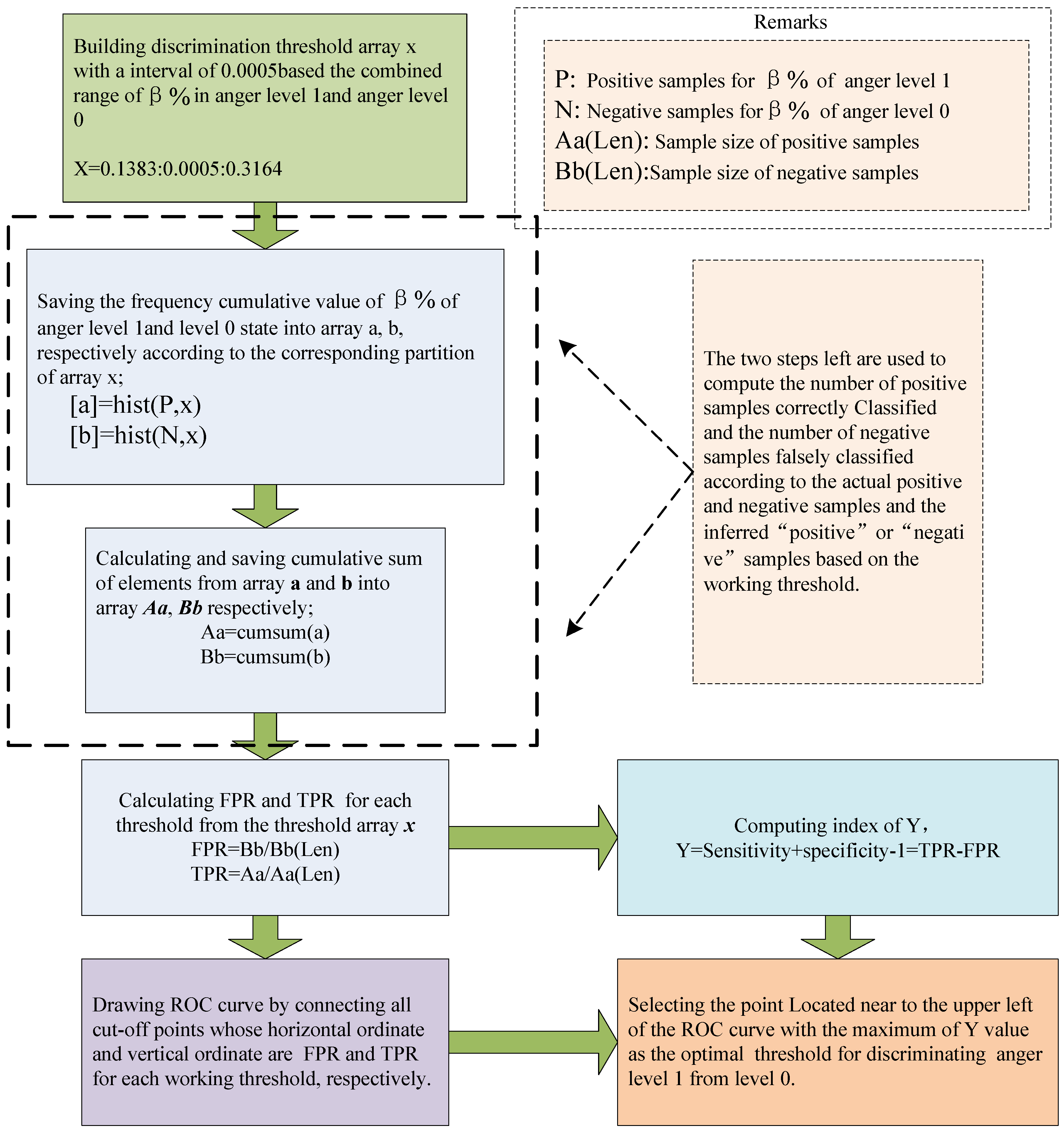
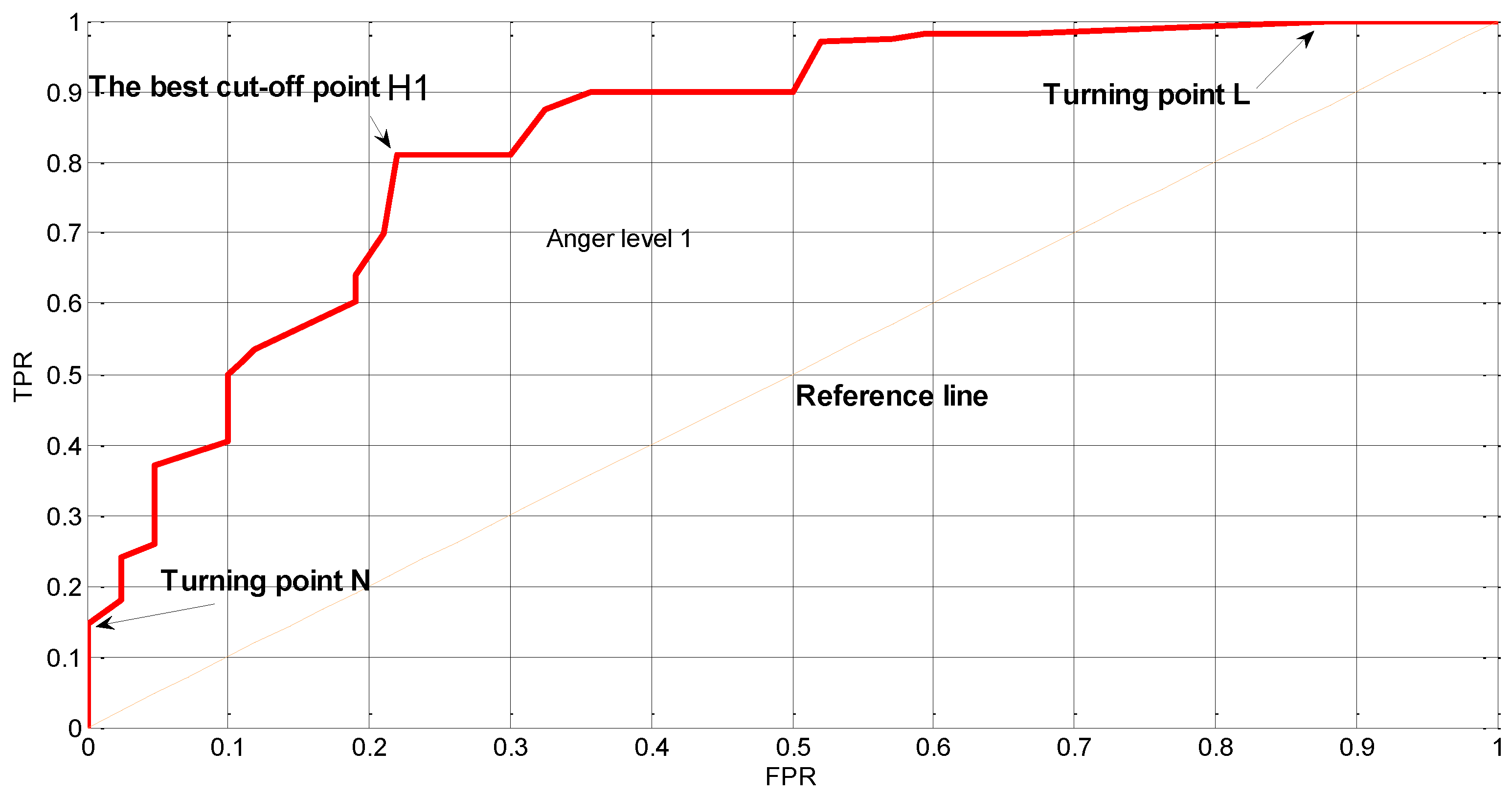
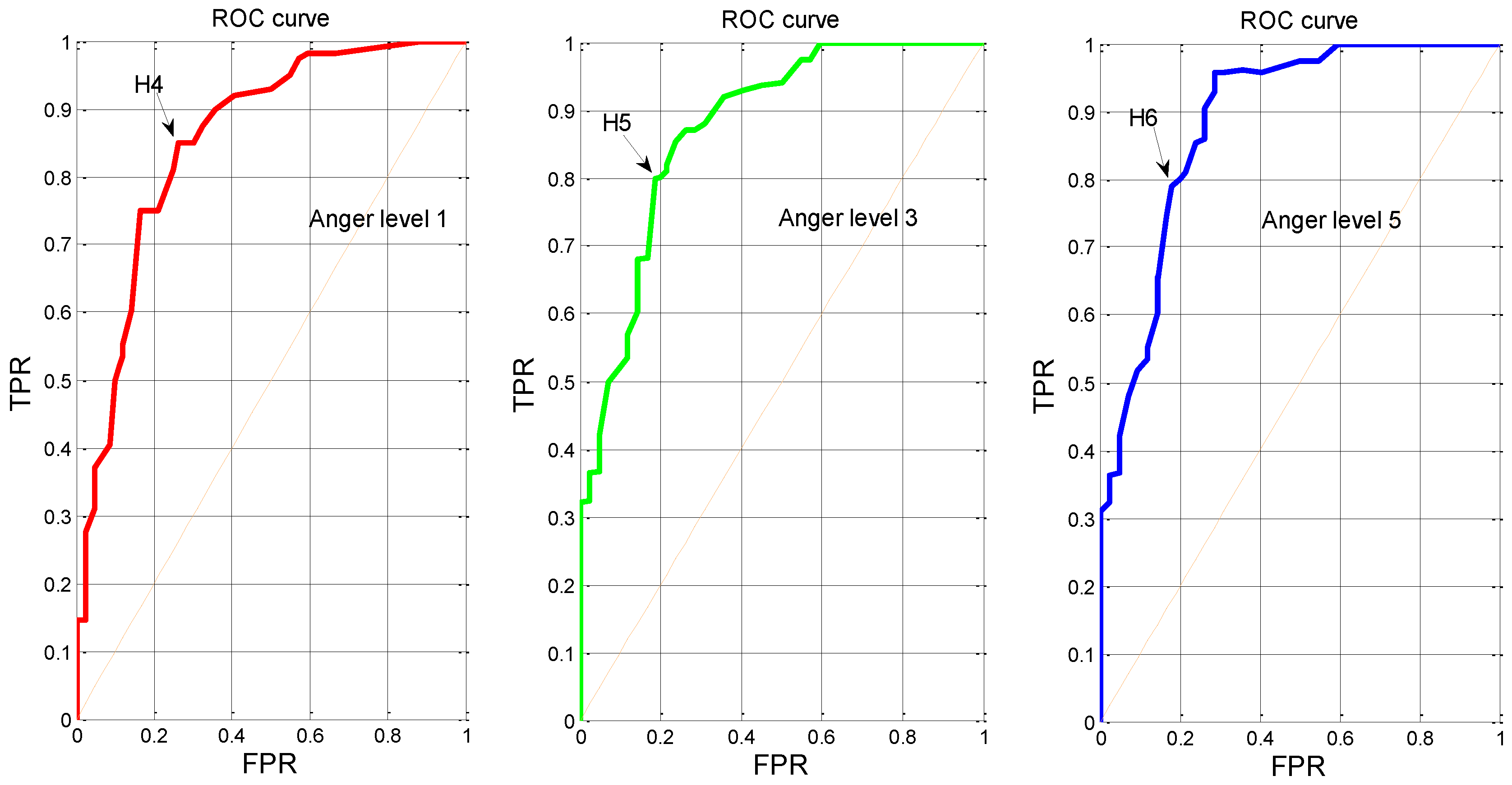
4.2. Determining Optimal Threshold by Drawing ROC Curve
5. Results
5.1. The Optimal Threshold for Discriminating Driving Anger Level 1 from Level 0
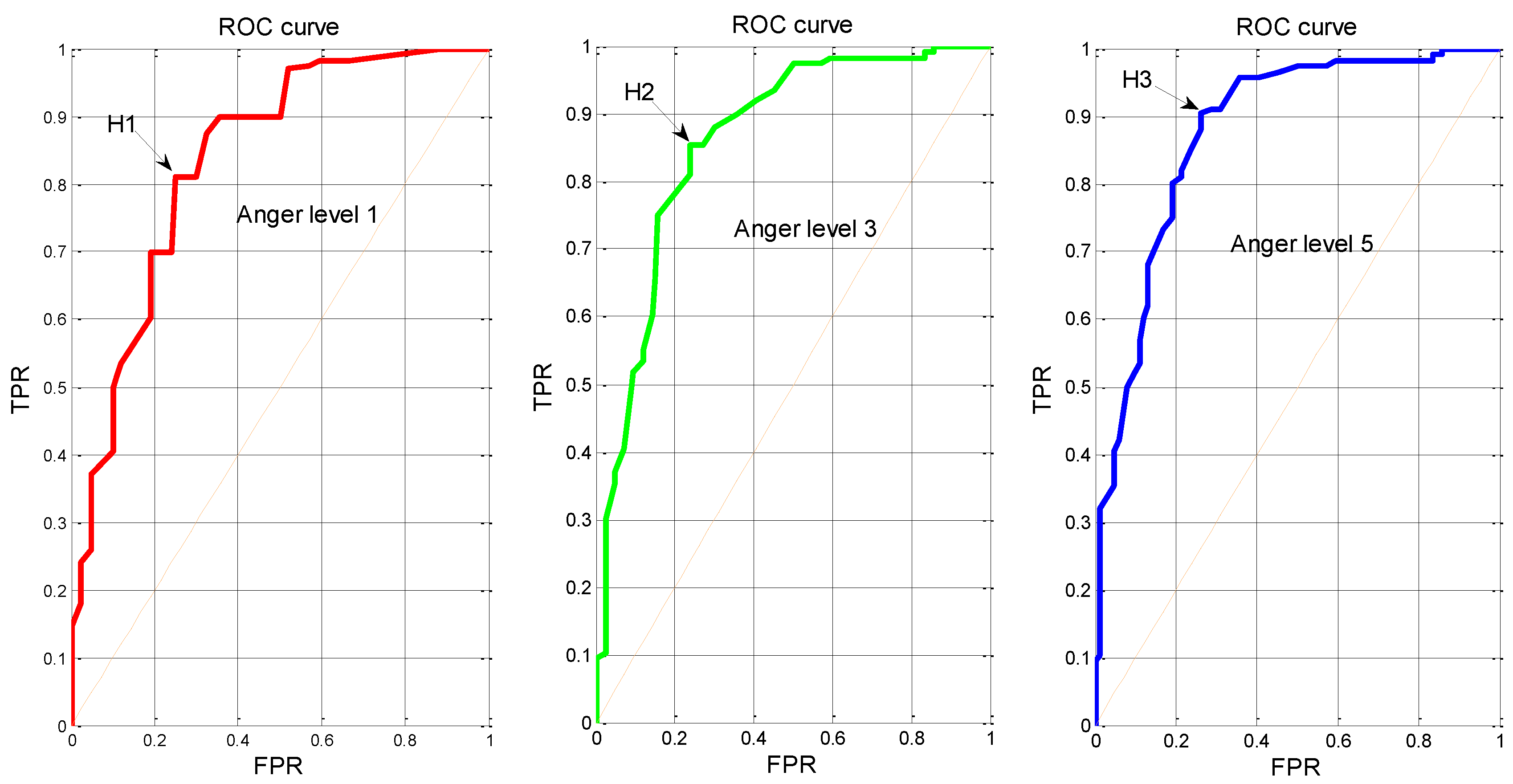
5.2. The Optimal Thresholds for Discriminating Anger States with Different Intensity
5.3. Verification of the Optimal Thresholds for Different-Intensity Anger States
6. Discussions and Conclusions
Acknowledgments
Author Contributions
Conflicts of Interest
References
- Wu, C.; Lei, H. Review on the study of motorists’ driving anger. China Saf. Sci. J. 2010, 20, 3–8. [Google Scholar]
- National Highway Traffic Safety Administration (NHTSA). Traffic Safety Facts: A Compilation of Motor Vehicle Crash Data from the Fatality Analysis Reporting System and the General Estimates System; U.S. Department of Transportation: Washington, DC, USA, 2011.
- Lei, H. The Characteristics of Angry Driving Behaviors and Its Effects on Traffic Safety. Master’s Thesis, Wuhan University of Technology, Wuhan, China, 2011. [Google Scholar]
- Dahlen, E.R.; Martin, R.C.; Ragan, K.; Kuhlman, M. Driving anger, sensation seeking, impulsiveness, and boredom proneness in the prediction of unsafe driving. Accid. Anal. Prev. 2005, 37, 341–348. [Google Scholar] [CrossRef] [PubMed]
- Sheila, S.; Alanna, M.; Mohammad, E.; Mohammad, K.; Karen, W. Aggressive driving and road rage behaviors on freeways in San Diego, California: Spatial and temporal analyses of observed and reported variations. Transp. Res. Rec. 2000, 1724, 7–13. [Google Scholar]
- Lajunen, T.; Parker, D. Are aggressive people aggressive drivers? A study of the relationship between self-reported general aggressiveness, driver anger and aggressive driving. Accid. Anal. Prev. 2001, 33, 243–255. [Google Scholar] [CrossRef]
- Zhang, D.; Wan, B.; Ming, D. Research progress on emotion recognition based on physiological signals. J. Biomed. Eng. 2015, 32, 229–234. [Google Scholar]
- Elena, S.; Songül, A. A facial component-based system for emotion classification. Turk. J. Electr. Eng. Comput. Sci. 2016, 24, 1663–1673. [Google Scholar]
- Wang, J.; Gong, Y. Normalizing multi-subject variation for drivers’ emotion recognition. In Proceedings of the IEEE International Conference on Multimedia and Expo, New York, NY, USA, 28 June–3 July 2009; pp. 354–357.
- Katsis, C.; Goletsis, Y.; Rigas, G.; Fotiadis, D. A wearable system for the affective monitoring of car racing drivers during simulated conditions. Transp. Res. C 2011, 19, 541–551. [Google Scholar] [CrossRef]
- Sibsambhu, K.; Bhagat, M.; Routra, A. EEG signal analysis for the assessment and quantification of driver’s fatigue. Transp. Res. F 2010, 13, 297–306. [Google Scholar]
- Yuen, C.T.; San, W.S.; Seong, T.C.; Rizon, M. Classification of human emotions from EEG signals using statistical features and neural network. Int. J. Integr. Eng. 2011, 1, 71–79. [Google Scholar]
- Choi, J.-S.; Bang, J.W.; Heo, H.; Park, K.R. Evaluation of Fear Using Nonintrusive Measurement of Multimodal Sensors. Sensors 2015, 15, 17507–17533. [Google Scholar] [CrossRef] [PubMed]
- Schaaff, K.; Schultz, T. Towards emotion recognition from electroencephalographic signals. In Proceedings of the 3rd International Conference on Affective Computing and Intelligent Interaction and Workshops, Amsterdam, The Netherlands, 9–12 September 2009; pp. 1–6.
- Wang, H.; Zhang, C.; Shi, T.; Wang, F.; Ma, S. Real-time EEG-based detection of fatigue driving danger for accident prediction. Int. J. Neural Syst. 2015, 25, 1550002. [Google Scholar] [CrossRef] [PubMed]
- Fu, R.; Wang, H.; Zhao, W. Dynamic driver fatigue detection using Hidden Markov model in real driving condition. Expert Syst. Appl. 2016, 63, 397–411. [Google Scholar] [CrossRef]
- Chai, R.; Naik, G.; Tran, Y.; Ling, S.; Craig, A.; Nguyen, H. Classification of driver fatigue in an electroencephalography-based countermeasure system with source separation module. In Proceedings of the 37th Annual International Conference of the IEEE Engineering in Medicine and Biology Society (EMBS), Milan, Italy, 25–29 August 2015; pp. 514–517.
- Chai, R.; Naik, G.; Nguyen, T.; Ling, S.; Tran, Y.; Craig, A.; Nguyen, H. Driver fatigue classification with independent component by entropy rate bound minimization analysis in an EEG-based system. IEEE J. Biomed. Health Inform. 2016, PP, 1. [Google Scholar] [CrossRef] [PubMed]
- Shuren, Q.; Zhong, J. Extraction of features in EEG signals with the non-stationary signal analysis technology. In Proceedings of the 26th Annual International Conference of the IEEE EMBS, San Francisco, CA, USA, 1–5 September 2004; pp. 349–352.
- Yamaguchi, C. Wavelet analysis of normal and epileptic EEG. In Proceedings of the Second Joint EMBS/BMES Conference, Huston, TX, USA, 23–26 October 2003.
- Khandoker, A.H.; Gubbi, J.; Palaniswami, M. Automated scoring of obstructive sleep apnea and hypopnea events using short-term electrocardiogram recordings. IEEE Trans. Inf. Technol. Biomed. 2009, 13, 1057–1067. [Google Scholar] [CrossRef] [PubMed]
- Murugappan, M.; Wali, M.K.; Ahmmd, R.B.; Murugappan, S. Subtractive fuzzy classifier based driver drowsiness levels classification using EEG. In Proceedings of the International Symposium on Communications and Signal Processing, Melmaruvathur, India, 3–5 April 2013; pp. 159–164.
- Shinar, D.; Compton, R.P. Aggressive driving: An observational study of driver, vehicle, and situational variables. Accid. Anal. Prev. 2004, 36, 429–437. [Google Scholar] [CrossRef]
- Feis, R.; Smith, S.; Filippini, N.; Douaud, G.; Dopper, E.G.; Heise, V.; Trachtenberg, A.J.; van Swieten, J.C.; van Buchem, M.A.; Rombouts, S.A.; et al. ICA-based artifact removal diminishes scan site differences in multi-center resting-state fMRI. Front. Neurosci. 2015, 9, 395. [Google Scholar] [CrossRef] [PubMed]
- Bilal, A.M.; Belkacem, F. News schemes for activity recognition systems using PCA-WSVM, ICA-WSVM, and LDA-WSVM. Information 2015, 6, 505–521. [Google Scholar]
- Kwon, Y.; Kim, K.; Tompkinet, J.; Kim, J.H.; Theobalt, C. Efficient learning of image super-resolution and compression artifact removal with semi-local Gaussian processes. IEEE Trans. Pattern Anal. Mach. Intell. 2015, 37, 1792–1805. [Google Scholar] [CrossRef] [PubMed]
- Bhardwaj, S.; Jadhav, P.; Adapa, B.; Acharyya, A.; Naik, G.R. Online and automated reliable system design to remove blink and muscle artifact in EEG. In Proceedings of the 37th Annual International Conference of the IEEE Engineering in Medicine and Biology Society (EMBS), Milan, Italy, 25–29 August 2015; pp. 6784–6787.
- Jadhav, P.; Shanamugan, D.; Chourasia, A.; Ghole, A.R.; Acharyya, A.A.; Naik, G. Automated detection and correction of eye blink and muscular artefacts in EEG signal for analysis of Autism Spectrum Disorder. In Proceedings of the 36th Annual International Conference of the IEEE Engineering in Medicine and Biology Society, Chicago, IL, USA, 27–31 August 2014; pp. 1881–1884.
- Rioul, O.; Vetterli, M. Wavelets and signal processing. IEEE Signal Process. Mag. 1991, 8, 14–38. [Google Scholar] [CrossRef]
- Mallat, S. A Wavelet Tour of Signal Processing, 2nd ed.; Academic Press: San Diego, CA, USA, 1999. [Google Scholar]
- Cheng, W.; Ni, Z.; Pan, X. Receiver operating characteristic curves to determine the optimal operating point and doubtable value interval. Mod. Prev. Med. 2005, 32, 729–731. [Google Scholar]
- Sun, C.; He, J.; Xiao, H. A new performance evaluation method based on ROC curve. Radar Sci. Technol. 2007, 5, 17–21. [Google Scholar]
- Bechtel, T.; Capineri, L.; Windsor, C.; Inagaki, M. Comparison of ROC curves for landmine detection by holographic radar with ROC data from other methods. In Proceedings of the 8th International Workshop on Advanced Ground Penetrating Radar, Florence, Italy, 7–10 July 2015; pp. 1–4.
- Zhao, X.H.; Du, H.J.; Rong, J. Research on identification method of fatigue driving based on ROC curves. J. Transp. Inf. Saf. 2014, 32, 88–94. [Google Scholar]
- Smart, R.G.; Stoduto, G.; Mann, R.E.; Adlaf, E.M. Road rage experience and behavior: Vehicle, exposure, and driver factors. Traffic Inj. Prev. 2004, 5, 343–348. [Google Scholar] [CrossRef] [PubMed]
- Deffenbacher, J.L. Anger, aggression, and risky behavior on the road: A preliminary study of urban and rural differences. J. Appl. Soc. Psychol. 2008, 38, 22–36. [Google Scholar] [CrossRef]
- Zhong, M.; Wu, P.; Peng, J. Study on an emotional state recognition technology based on drivers’ EEGs. China Saf. Sci. J. 2011, 21, 64–69. [Google Scholar]
- Xiang, J.; Cao, R.; Li, L. Emotion recognition based on the sample entropy of EEG. Bio Med. Mater. Eng. 2014, 24, 1185–1192. [Google Scholar]
- Rebolledo-Mendez, G.; Angélica, R.; Sebastian, P.; Domingo, M.C.; Skrypchuk, L. Developing a body sensor network to detect emotions during driving. IEEE Trans. Intell. Transp. Syst. 2014, 15, 1850–1854. [Google Scholar] [CrossRef]


| Parameter | Anger Intensity | p Value | |||
|---|---|---|---|---|---|
| None | Low | Moderate | High | ||
| δ% | 0.3328(0.0924) | 0.2956(0.0753) | 0.3236(0.0893) | 0.3178(0.0831) | 0.188 |
| θ% | 0.2812(0.0746) | 0.2379(0.0638) | 0.1784(0.0482) | 0.1465(0.0387) | 0.036 |
| α% | 0.1631(0.0472) | 0.1746(0.0526) | 0.1675(0.0463) | 0.1405(0.0394) | 0.237 |
| β% | 0.2034(0.0584) | 0.2818(0.0682) | 0.3443(0.0784) | 0.3825(0.0926) | 0.024 |
| Anger Level | Indicator | AUC | Std. Error | Asymptotic Sig. | 95% Confidence Interval | |
|---|---|---|---|---|---|---|
| Lower Limit | Upper Limit | |||||
| level 1 | θ% | 0.8072 | 0.0273 | 0.038 | 0.7562 | 0.8548 |
| β% | 0.7914 | 0.0261 | 0.042 | 0.7513 | 0.8416 | |
| level 3 | θ% | 0.8276 | 0.0284 | 0.032 | 0.7826 | 0.8732 |
| β% | 0.8168 | 0.0276 | 0.029 | 0.7682 | 0.8673 | |
| level 5 | θ% | 0.8635 | 0.0325 | 0.024 | 0.8147 | 0.9129 |
| β% | 0.8587 | 0.0318 | 0.026 | 0.8092 | 0.8994 | |
| Anger Level | Indicator | TPR | FPR | Best Cut-off Point |
|---|---|---|---|---|
| level 1 | θ% | 0.7506 | 0.1652 | 0.2183 |
| β% | 0.8103 | 0.2214 | 0.2586 | |
| level 3 | θ% | 0.8009 | 0.1864 | 0.1539 |
| β% | 0.8534 | 0.2381 | 0.3269 | |
| level 5 | θ% | 0.7890 | 0.1780 | 0.1216 |
| β% | 0.9052 | 0.2619 | 0.3674 |
| Anger Intensity | None Anger | Low | Moderate | High |
|---|---|---|---|---|
| Level < 1 | 1 ≤ Anger Level < 3 | 3 ≤ Anger Level < 5 | Anger Level ≥ 5 | |
| θ% | [0.2183,1) | [0.1539,0.2183) | [0.1216,0.1539) | (0,0.1216) |
| β% | (0,0.2586) | [0.2586,0.3269) | [0.3269,0.3674) | [0.3674,1) |
| Indicators | Classified as None | Classified as Low | Classified as Moderate | Classified as High | Total | |
|---|---|---|---|---|---|---|
| θ% | None | 302 | 56 | 22 | 0 | 380 |
| Low | 32 | 212 | 40 | 16 | 300 | |
| Moderate | 10 | 20 | 146 | 24 | 200 | |
| High | 2 | 8 | 18 | 92 | 120 | |
| β% | None | 320 | 46 | 16 | 2 | 380 |
| Low | 24 | 228 | 34 | 14 | 300 | |
| Moderate | 8 | 16 | 156 | 20 | 200 | |
| High | 0 | 6 | 16 | 98 | 120 |
| Indicators | Recall/TPR | Precision | F1 | Acc | |
|---|---|---|---|---|---|
| θ% | None | 79.47% | 87.28% | 83.19% | 75.20% |
| Low | 70.67% | 71.62% | 71.14% | ||
| Moderate | 73.02% | 64.60% | 68.54% | ||
| High | 76.67% | 69.70% | 73.02% | ||
| β% | None | 84.21% | 90.91% | 87.43% | 80.21% |
| Low | 76.05% | 77.03% | 76.51% | ||
| Moderate | 78.08% | 70.27% | 73.93% | ||
| High | 81.66% | 73.13% | 77.16% |
© 2016 by the authors; licensee MDPI, Basel, Switzerland. This article is an open access article distributed under the terms and conditions of the Creative Commons Attribution (CC-BY) license (http://creativecommons.org/licenses/by/4.0/).
Share and Cite
Wan, P.; Wu, C.; Lin, Y.; Ma, X. Optimal Threshold Determination for Discriminating Driving Anger Intensity Based on EEG Wavelet Features and ROC Curve Analysis. Information 2016, 7, 52. https://doi.org/10.3390/info7030052
Wan P, Wu C, Lin Y, Ma X. Optimal Threshold Determination for Discriminating Driving Anger Intensity Based on EEG Wavelet Features and ROC Curve Analysis. Information. 2016; 7(3):52. https://doi.org/10.3390/info7030052
Chicago/Turabian StyleWan, Ping, Chaozhong Wu, Yingzi Lin, and Xiaofeng Ma. 2016. "Optimal Threshold Determination for Discriminating Driving Anger Intensity Based on EEG Wavelet Features and ROC Curve Analysis" Information 7, no. 3: 52. https://doi.org/10.3390/info7030052
APA StyleWan, P., Wu, C., Lin, Y., & Ma, X. (2016). Optimal Threshold Determination for Discriminating Driving Anger Intensity Based on EEG Wavelet Features and ROC Curve Analysis. Information, 7(3), 52. https://doi.org/10.3390/info7030052