Abstract
Deep learning is used in various applications due to its advantages over traditional Machine Learning (ML) approaches in tasks encompassing complex pattern learning, automatic feature extraction, scalability, adaptability, and performance in general. This paper proposes an end-to-end (E2E) delay estimation method for 5G networks through deep learning (DL) techniques based on Gaussian Mixture Models (GMM). In the first step, the components of a GMM are estimated through the Expectation-Maximization (EM) algorithm and are subsequently used as labeled data in a supervised deep learning stage. A multi-layer neural network model is trained using the labeled data and assuming different numbers of E2E delay observations for each training sample. The accuracy and computation time of the proposed deep learning estimator based on the Gaussian Mixture Model (DLEGMM) are evaluated for different 5G network scenarios. The simulation results show that the DLEGMM outperforms the GMM method based on the EM algorithm, in terms of the accuracy of the E2E delay estimates, although requiring a higher computation time. The estimation method is characterized for different 5G scenarios, and when compared to GMM, DLEGMM reduces the mean squared error (MSE) obtained with GMM between 1.7 to 2.6 times.
1. Introduction
Network analytics enables network operators to utilize practical models to troubleshoot configuration issues, improve network efficiency, reduce operational expenses, detect potential security threats, and plan network development [1]. Quality-of-service (QoS) metrics serve as performance indicators of network status, and network operators utilize various methods to enhance user experiences by improving QoS metrics. For example, 5G cellular networks use resource allocation and power control to ensure a robust connection with minimal delay for Device-to-Device (D2D) communications [2].
As 5G networks continue to be deployed and new applications emerge, the ability to accurately predict and estimate end-to-end (E2E) delay is of high importance for ensuring optimal network performance and user experience. The E2E delay is one of the most critical QoS metrics directly related to user experience and quality, being defined as the time required to transfer a packet from one endpoint to another. From a network management perspective, identifying the network’s E2E delay profile is critical for evaluating its suitability in supporting different delay-constrained services over time [3]. The understanding of the E2E delay probabilistic features is essential for efficient network management and improved QoS for diverse service requirements, including but not limited to throughput, reliability, and time sensitivity.
In 5G networks, the diversity of services demands different E2E delay requirements. For example, Ultra-Reliable Low Latency Communication (URLLC) applications require extremely low latency to ensure high reliability, while applications such as opportunistic sensing do not require such stringent latency requirements [4]. Operators must comprehensively understand the network’s E2E delay profile to optimize their networks and ensure smooth operations, although the characterization of the E2E delay involves parameterizing different delay patterns that might change significantly over time [5]. The probabilistic models can help network operators design delay management strategies that fulfill the specific needs of each service [6]. One of the critical challenges in the characterization of the E2E delay through various distribution models is determining which distributions represent the experimental data collected over time. The Gaussian Mixture Model (GMM) is a well-fitted candidate for estimating the delay distribution when it does not follow a single known Probability Density Function (PDF). The GMM can capture the data’s underlying distribution by estimating each Gaussian component’s parameters, including the mean, variance, and mixture weights. The parameters of GMM are often estimated by the Expectation-Maximization (EM) approach, an iterative algorithm that maximizes the likelihood of the data provided to the model [7].
In our work in [8], we proposed a method for estimating the E2E delay in 5G networks using the GMM based on the EM algorithm. However, its accuracy is quite limited and our motivation in this paper is to introduce an innovative methodology, a deep learning estimator based on the Gaussian Mixture Model (DLEGMM), capable of increasing the GMM accuracy achieved in [8]. The main contribution of DLEGMM relies on the use of deep learning to improve the accuracy of the estimation of the E2E delay distribution parameters based on a short amount of E2E delay samples. In DLEGMM, we use the parameters identified with the EM algorithm to generate labeled training data for a deep learning model. We provide a detailed study of the estimation accuracy and computation time of DLEGMM for different scenarios, confirming its higher accuracy. The main contributions of this work include:
- A methodology to label 5G E2E delay data according to the GMM parameters obtained with the EM algorithm for different amounts of observed values to be used in the estimation;
- The description of an estimation methodology that uses the 5G E2E labeled data in a deep learning model capable of computing the GMM parameters;
- The evaluation of the proposed estimation methodology in terms of accuracy and computation time and its comparison with the estimation approach in [8] that adopts the EM algorithm only.
In this work, we estimate the E2E delay of a 5G Network measured as the one-way direction E2E delay between the user equipment device and the network (upload) or in the reverse direction (download). To this end, the focus of our work is centered on the E2E delay values measured between the user equipment and the 5G network. We only consider the 5G access network to which the user equipment is connected. The goal of our research is to estimate the E2E delay of the 5G network because it can effectively change due to traffic distribution, resource allocation policies, etc. We address the delay of the access network because it is a critical resource that can be estimated in advance by the end user’s device to evaluate if the access network can support a specific service or if another access network should be used instead. The proposed methodology is evaluated by characterizing the impact of adopting a small number of E2E delay samples (from 5 to 120) on the delay estimation process through different deep learning models and the GMM model. By using a small number of samples, the estimation methodology can adapt more quickly to rapid changes in the delay statistics and it is an advantage of the proposed methodology.
2. Literature Review
In the rapidly evolving world of telecommunications, the advent of 5G technology promises lightning-fast data transmission and ultra-low latency communications. However, ensuring a seamless end-user experience in 5G networks requires accurate prediction and management of E2E delay. In the 5G networks context, the E2E delay refers to the time taken for data to travel from the source to the destination, encompassing all the intermediary processes. E2E delay has been employed as a key performance indicator (KPI) parameter that directly impacts the user experience quality and latency-sensitive applications [9,10]. The URLLC supported by 5G technology opens up new opportunities for implementing applications such as autonomous vehicles, virtual reality, securing the Internet of Things (IoT), and industrial automation [11].
Designing and optimizing E2E delay in networks to meet the stringent latency requirements of the applications presents significant challenges in achieving the desired level of delay [12]. Predicting E2E delay is crucial for optimizing network performance, enhancing user experience, and ensuring efficient data transmission. Considerable research endeavors have been focused on investigating E2E delay networks within the scope of 5G. These topics already explored cover network architecture [13], traffic management [14], resource allocation [15], and protocol design [16]. These studies aim to minimize overall delay by addressing factors such as propagation delays, processing delays, and queuing delays across various network layers.
The accurate prediction and estimation of end-to-end delay in 5G networks remain a challenging research problem due to the complexity of the network architecture, the dynamic nature of network traffic, the presence of various sources of delay, and the complexity of the estimation and prediction algorithms. The models and techniques already proposed for predicting and estimating end-to-end delay in 5G networks can be classified into four groups:
- Analytical modeling techniques, such as queuing theory [17,18] and network calculus [19], capture the stochastic behavior of the E2E connecting path through theoretical models, which are subsequently adopted for predicting purposes;
- Statistical modeling approaches different from queuing models have also been proposed for predicting E2E delay in 5G networks [8,20,21]. These approaches typically use statistical techniques such as regression analysis, time-series analysis, and probabilistic modeling to estimate the relation between network parameters and delay performance;
- Network simulation: Network simulation tools such as ns-3 and OPNET have been used to simulate and analyze the performance of 5G networks. These tools allow researchers to model the network architecture, traffic patterns, and other key parameters, and analyze the impact on end-to-end delay performance;
- Various deep learning (DL) models have been adopted for E2E delay estimation [22]. These models capture the complex temporal dependencies and non-linear relationships present in the network data. The models are trained on large-scale datasets comprising network measurements, traffic patterns, network topology, and other relevant features.
Overall, the state-of-the-art 5G end-to-end delay prediction and estimation is rapidly evolving, with ongoing research aimed at developing more accurate and efficient models and techniques for predicting delay performance in 5G networks.
In our work, we adopt a statistical modeling approach based on Gaussian Mixture models to label raw data that is further used to train DL models. Consequently, our approach takes advantage of two different types of models, which is the main contribution of our work.
3. System Model
In this work, we adopt the 5G Campus dataset [23] as a primary source of 5G E2E delay samples. The Wireshark software is adopted in this dataset to capture all received and transmitted packets in a specific Network Interface Card (NIC). The collection of data in the 5G Campus dataset is accomplished through the tracking of timestamped packets. This dataset encompasses various subsets consisting of Standalone (SA) and Non-Standalone (NSA) 5G technologies, transmitting data in both upload and download directions and featuring varying packet sizes and data rates. Comprehensive information regarding this dataset and its utilization in our research can be found in [8]. In our work, we consider these subsets as offline or online 5G network data.
The system model block diagram followed in the DLEGMM approach is illustrated in Figure 1.
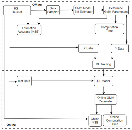
Figure 1.
DLEGMM system model.
In the offline stage, the 5G Dataset is used to determine the GMM parameters. The dataset samples are used by the “GMM Model EM Estimator” to determine the parameters of the GMM model through the EM algorithm and the resulting parameters are evaluated in terms of accuracy of the GMM estimation by the Mean Squared Error (MSE) between the empirical data and the estimated distributions in the “Estimation Accuracy (MSE)” block. Additionally, the estimation time is evaluated by measuring the computation time needed to determine the GMM parameters for a specific set of samples, which is recorded after executing the estimation process and measured in the “Computation Time” block.
The 5G E2E dataset is also divided in consecutive sets of E2E delay samples, where each sample is an E2E delay value. The multiple X datasets are separated into training and test data at a rate of and , respectively. The training data is used as input for the training process of the DL model and is provided by the “X Data” block. The data from the “X Data” block is labeled with the results of the GMM parameters computed in the offline mode, represented by the “Y Data” block, and both “X Data” and “Y Data” blocks are used as “Supervised Data” to train the DL estimation model in the “DL Training” block.
In the online stage, after performing the training process of the deep learning model during the offline stage, represented in the “DL Training block”, the test data is used as input data in the “DL Model”, which computes the new GMM parameters’ value based on online “Test Data”. Similarly to the offline assessment, the online stage is also evaluated in terms of MSE of the accuracy and estimation computation time.
It is worth noting that while the whole dataset is used to determine the GMM parameters used to label the different x sets, the DL model only requires a smaller number of E2E delay values, i.e., T values in X, to determine the GMM parameters. This procedure means that a much smaller number of E2E delay values is required by the DL model, thus increasing its computation time. Additionally, because each set X is labeled with the GMM parameters obtained for the entire dataset and used to train the DL model, the accuracy of the DL model increases when compared to the estimation obtained with the EM algorithm for the same number (T) of E2E delay values. This is seen as the main advantage of the proposed methodology and is the focus of the next sections.
4. Estimation Methodology
This section provides a detailed description of the estimation process. During the offline stage, all the collected data in the 5G Dataset is used to determine the GMM parameters. The EM algorithm is adopted to estimate the GMM parameters using all E2E delay samples in the 5G Dataset. The EM algorithm is an iterative process with two steps: the Expectation (E) and the Maximization (M) steps. In the E step, the posterior probability of each data point belonging to each GMM component is calculated using Bayes’ rule and the current parameter estimates. The M step then updates the GMM parameters based on the posterior probabilities calculated in the E step, including the mean, covariance, and weight of each GMM component. This process is repeated until convergence, determined by a pre-specified tolerance level. Once the GMM parameters are estimated, the estimated data is compared to the real dataset to determine the Mean Squared Error (MSE) and processing time for different GMM components and sample sizes. A detailed procedure for GMM parameter estimation for 5G E2E delay datasets in the offline estimation can be found in [8]. The GMM parameter estimation results obtained with the EM algorithm are used to label each sample set X and subsequently used as supervised data to train a DL model consisting of a Neural network. Regarding the GMM model, we have adopted eight GMM components, which lead to high accuracy, as reported in [8]. By adopting eight GMM components, and since each component is described by three parameters, mean (), standard deviation (), and weight (W), the eight components are described by twenty-four parameters. The twenty-four parameters computed with the EM algorithm for three different scenarios, further described in Section 5, are shown in Table 1.

Table 1.
Estimated parameters for Scenarios 1, 2, and 3 presented in Section 5.
The offline stage also includes the training of the DL model. The neural network adopted in the DL model consists of multiple layers that perform various functions to extract relevant features and model complex relations among inputs and outputs. The 5G E2E delay training data are used in the deep-learning architecture to train the neural network. The training data is reshaped into vectors X of length T, with . The different values of T represent different numbers of inputs adopted in the estimation method. For each set of samples X of length T we use the 24 values obtained from the EM algorithm, denoted as . The 24 values in Y are used to label each X dataset so that the pair can be used as supervised data for training purposes.
The neural network proposed as the DL model is composed of eight layers, including the input and output layers. The number of neurons in each layer is shown in Figure 2.
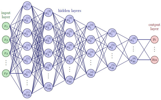
Figure 2.
DLEGMM neural network structure with the input layer X, output layer Y, and six hidden layers.
The network consisted of six hidden layers, with , and 30 neurons, respectively. The ReLU activation function was used for all of these layers. The output layer is of length 24, representing the eight GMM components with three parameters each, and uses the linear activation function.
Regarding the training of the neural network, each layer in the network is connected to the next layer, and the output of each layer is the input of the subsequent one. The output of the last layer is the output of the network. The bias provides constant input values to each network layer. Equation (1) represents one of the neurons of the network,
where f represents the activation function, represents the output from layer l, and neuron i in that layer, represents the weight of the connection between neuron i in layer l and neuron j in layer , and represents the bias of neuron i in layer l. The network weights are randomly initialized before training. Each data input X formed from the original dataset serves as the input of the neural network, and the output is computed using the neural network training algorithm. The loss function f determines the degree of proximity between the network’s output and the target output given by the values in Table 1. The MSE used as the loss function of the neural network during the training process is given by
where N represents the number of inputs X used in the training batch, represents the desired output for the ith input, and represents the output of the network for the i-th input. The loss function is used by the backpropagation algorithm to determine the network weights and bias by minimizing the loss function concerning the multiple weights. The backpropagation algorithm uses the chain rule of calculus. Equation (3) represents the regular Stochastic Gradient Descent (SGD) rule to update the network weights,
The variable is the weight to update at time k, L is the loss function, and is the learning rate. The term represents the gradient of the loss function for the weight w. Instead of regular SGD, we used a variant called Adaptive Moment (Adam) estimation [24]. Adam computes individual adaptive learning rates for different parameters using estimates of the first and second moments of the gradients as follows
where and are the first and second moments of the gradients, respectively. and are hyperparameters that control the exponential decay rates of the moment estimates. is the learning rate, and is a threshold to prevent division by zero. The Adam optimization algorithm was parameterized with , , a learning rate of , and . The input data were reshaped into vectors of length to train eight different networks that adopt a different number of input E2E delay samples.
The neural network is updated online based on the real-time data gathered during testing. In the online estimation stage, the trained neural network is used to predict the outputs of the test data, which serves as an online data stream. The predictions of the GMM model obtained with the neural network are used to represent the estimated cumulative distribution function (CDF) of the E2E delay over , discrete codomain points. The estimated CDF is compared through the MSE with the CDF of the empirical dataset in discrete codomain points as follows
The computing time to obtain each estimated CDF is also obtained at the end of the estimation process.
5. Performance Evaluation
This section aims to evaluate the estimation performance using the E2E delay data available in the 5G Campus dataset [23]. In this dataset, each sub-dataset is distinguished from others by different data collection conditions in terms of network architecture (Standalone (SA) and Non-Standalone (NSA)), delay measurements (RAN/Core), stream direction (Download/Upload), packet size (128/256/512/1024/2048 bytes), and packet rate (10/100/1000/10,000/100,000 packets per second).
Table 2 identifies the three scenarios adopted in the estimation performance evaluation, which can be found in three different 5G Campus sub-datasets. These scenarios were chosen due to their ability to showcase the accuracy of the proposed estimation method.
Table 2.
The 5G Campus dataset scenarios adopted in the performance evaluation.
The core E2E delay in the NSA topology is collected in the download stream direction in all selected scenarios. The packet size used for analysis is 1024 bytes, and data rates of 10, 100, and 1000 packets per second were used to generate the network traffic.
As mentioned before, the MSE is the main parameter adopted in this work to evaluate the performance of estimation methods. The MSE in (7) is computed for all scenarios and considering the different number of estimator inputs, i.e., . In what follows, we use the term inputs to refer to the number of E2E delay samples, i.e., T—the length of the vector of samples, used in the estimation process. The MSE values for different inputs and scenarios are summarized in Table 3 and plotted in Figure 3. In addition to the three scenarios, we included the MSE obtained with the GMM estimation model, identified as “Scenario 1-GMM”, for comparison purposes. We highlight that the results labeled as “Scenario 1-GMM” are obtained with the EM algorithm and serve as a benchmark.
Table 3.
MSE for different scenarios and number of inputs (T).
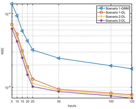
Figure 3.
MSE for different scenarios and inputs (T).
For the same number of GMM components, the MSE decreases as the number of inputs increases, which means that a lower error is achieved when more inputs are used in the estimation process. In addition, the MSE value decreases as more probing packets are sent per second while maintaining the input size, which indicates that a higher sampling rate slightly decreases the MSE. Regarding the comparison with the GMM estimation method, the results indicate that DLEGMM can reduce the MSE between 1.7 to 2.6 times, which shows the superiority of the proposed method. Regarding the justification of the achieved results, we highlight that for GMM estimation the EM algorithm needs a high number of samples to reduce the MSE. However, because DLEGMM was trained with small sets of data, labeled with the GMM parameters obtained with the EM algorithm for the entire dataset, the estimation of the GMM parameters is more accurate when using the DLEGMM than when using the EM algorithm for the same amount of samples/inputs.
On the other hand, the estimation computation time is one of the most valuable parameters because it indicates the time needed to compute a new estimation on the trained neural network. The computation time is presented in Table 4 and plotted in Figure 4 for the different scenarios and number of inputs (T). The estimation computation time is also compared with the GMM estimation computation time, identified in Table 4 and Figure 4 by the label “Scenario 1-GMM”. As a general trend, the computation time increases with the number of inputs because the neural network model complexity also increases with the number of inputs. Regarding the GMM computation time, we observe that the GMM estimator performs better in terms of computation time but its accuracy is not that high, as shown in the results in Table 3 and Figure 3. The results also show that GMM’s computation time is more influenced by the number of inputs than the DLEGMM model and for a higher number of inputs the GMM computation time becomes more close to the DLEGMM computation time, although always lower.
Table 4.
Computation time [ms] for different scenarios and number of inputs (T).
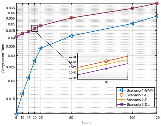
Figure 4.
Computation time (in milliseconds) for different scenarios and inputs (T).
As a final remark, the performance evaluation results indicate that increasing the number of inputs and packet probing rates leads to more precise modeling, which is advantageous to decrease the MSE. Furthermore, the MSE is more impacted by the number of inputs than the packet probing sampling rate adopted in each scenario. However, the increase in the number of inputs results in a higher computational time, although more advantageous for DLEGMM because it is less influenced by the number of inputs. Overall, the results from Figure 3 and Figure 4 highlight the trade-off between MSE and the estimation computation time and suggest that a balance must be struck to achieve the required performance.
6. Conclusions
This paper proposed the DLEGMM approach to estimate 5G E2E delay. The proposed method relies on the training of a neural network with a supervised learning approach employing supervised data computed with the EM algorithm to estimate the parameters of 8 GMM components. The DLEGMM approach is evaluated using different input sizes and scenarios, and the results show that the MSE decreases with an increase in the number of inputs. However, the computation time increases with the number of inputs and dataset size. The study highlights the importance of selecting the best-suited estimation method based on the specific application’s requirements and tradeoffs between accuracy and computation time. Additionally, the comparison highlights the superiority of DLEGMM in terms of estimation accuracy, although it requires a higher computation time when compared to the GMM estimation model when only a small number of E2E delay samples are adopted. However, as the number of E2E delay samples used in the estimation increases the computation time of the DLEGMM is similar to or even shorter than the GMM EM-based estimation model and DLEGMM can present better performance in terms of both estimation accuracy and computation time.
Author Contributions
Conceptualization, R.O.; methodology, D.F. and R.O.; software, D.F.; validation, D.F. and R.O.; writing—review and editing, D.F. and R.O. All authors have read and agreed to the published version of the manuscript.
Funding
This work was supported by the Fundação para a Ciência e Tecnologia through the projects CELL-LESS6G (2022.08786.PTDC) and UIDB/50008/2020.
Data Availability Statement
Data are contained within the article.
Conflicts of Interest
The authors declare no conflict of interest.
References
- Pržulj, N.; Malod-Dognin, N. Network Analytics in the Age of Big Data. Science 2016, 353, 123–124. [Google Scholar] [CrossRef] [PubMed]
- Pandey, K.; Arya, R. Robust Distributed Power Control with Resource Allocation in D2D Communication Network for 5G-IoT Communication System. Int. J. Comput. Netw. Inf. Secur. 2022, 14, 73–81. [Google Scholar] [CrossRef]
- Oleiwi, S.S.; Mohammed, G.N.; Al_barazanchi, I. Mitigation of Packet Loss with End-to-End Delay in Wireless Body Area Network Applications. Int. J. Electr. Comput. Eng. 2022, 12, 460. [Google Scholar] [CrossRef]
- Afolabi, I.; Taleb, T.; Samdanis, K.; Ksentini, A.; Flinck, H. Network Slicing and Softwarization: A Survey on Principles, Enabling Technologies, and Solutions. IEEE Commun. Surv. Tutor. 2018, 20, 2429–2453. [Google Scholar] [CrossRef]
- Ye, Q.; Zhuang, W.; Li, X.; Rao, J. End-to-End Delay Modeling for Embedded VNF Chains in 5G Core Networks. IEEE Internet Things J. 2019, 6, 692–704. [Google Scholar] [CrossRef]
- Banavalikar, B.G. Quality of Service (QoS) for Multi-Tenant-Aware Overlay Virtual Networks. US Patent 10,177,936, 1 October 2015. [Google Scholar]
- Reynolds, D.A. Gaussian Mixture Models. Encycl. Biom. 2009, 741, 659–663. [Google Scholar]
- Fadhil, D.; Oliveira, R. Estimation of 5G Core and RAN End-to-End Delay through Gaussian Mixture Models. Computers 2022, 11, 184. [Google Scholar] [CrossRef]
- Yuan, X.; Wu, M.; Wang, Z.; Zhu, Y.; Ma, M.; Guo, J.; Zhang, Z.L.; Zhu, W. Understanding 5G performance for real-world services: A content provider’s perspective. In Proceedings of the ACM SIGCOMM 2022 Conference, Amsterdam, The Netherlands, 22–26 August 2022; pp. 101–113. [Google Scholar]
- Chinchilla-Romero, L.; Prados-Garzon, J.; Ameigeiras, P.; Muñoz, P.; Lopez-Soler, J.M. 5G infrastructure network slicing: E2E mean delay model and effectiveness assessment to reduce downtimes in industry 4.0. Sensors 2021, 22, 229. [Google Scholar] [CrossRef] [PubMed]
- Maroufi, M.; Abdolee, R.; Tazekand, B.M.; Mortezavi, S.A. Lightweight Blockchain-Based Architecture for 5G Enabled IoT. IEEE Access 2023, 11, 60223–60239. [Google Scholar] [CrossRef]
- Herrera-Garcia, A.; Fortes, S.; Baena, E.; Mendoza, J.; Baena, C.; Barco, R. Modeling of Key Quality Indicators for End-to-End Network Management: Preparing for 5G. IEEE Veh. Technol. Mag. 2019, 14, 76–84. [Google Scholar] [CrossRef]
- Gupta, A.; Jha, R.K. A Survey of 5G Network: Architecture and Emerging Technologies. IEEE Access 2015, 3, 1206–1232. [Google Scholar] [CrossRef]
- Liu, J.; Wan, J.; Jia, D.; Zeng, B.; Li, D.; Hsu, C.H.; Chen, H. High-Efficiency Urban Traffic Management in Context-Aware Computing and 5G Communication. IEEE Commun. Mag. 2017, 55, 34–40. [Google Scholar] [CrossRef]
- Xu, Y.; Gui, G.; Gacanin, H.; Adachi, F. A survey on resource allocation for 5G heterogeneous networks: Current research, future trends, and challenges. IEEE Commun. Surv. Tutor. 2021, 23, 668–695. [Google Scholar] [CrossRef]
- Zhang, Z.; Chai, X.; Long, K.; Vasilakos, A.V.; Hanzo, L. Full duplex techniques for 5G networks: Self-interference cancellation, protocol design, and relay selection. IEEE Commun. Mag. 2015, 53, 128–137. [Google Scholar] [CrossRef]
- Diez, L.; Alba, A.M.; Kellerer, W.; Aguero, R. Flexible Functional Split and Fronthaul Delay: A Queuing-Based Model. IEEE Access 2021, 9, 151049–151066. [Google Scholar] [CrossRef]
- Fadhil, D.; Oliveira, R. A Novel Packet End-to-End Delay Estimation Method for Heterogeneous Networks. IEEE Access 2022, 10, 71387–71397. [Google Scholar] [CrossRef]
- Adamuz-Hinojosa, O.; Sciancalepore, V.; Ameigeiras, P.; Lopez-Soler, J.M.; Costa-Pérez, X. A Stochastic Network Calculus (SNC)-Based Model for Planning B5G uRLLC RAN Slices. IEEE Trans. Wirel. Commun. 2023, 22, 1250–1265. [Google Scholar] [CrossRef]
- Ahmed, A.H.; Hicks, S.; Riegler, M.A.; Elmokashfi, A. Predicting High Delays in Mobile Broadband Networks. IEEE Access 2021, 9, 168999–169013. [Google Scholar] [CrossRef]
- Fadhil, D.; Oliveira, R. Characterization of the End-to-End Delay in Heterogeneous Networks. In Proceedings of the 12th International Conference on Network of the Future (NoF), Coimbra, Portugal, 6–8 October 2021; pp. 1–5. [Google Scholar] [CrossRef]
- Ge, Z.; Hou, J.; Nayak, A. GNN-based End-to-end Delay Prediction in Software Defined Networking. In Proceedings of the 2022 18th International Conference on Distributed Computing in Sensor Systems (DCOSS), Los Angeles, CA, USA, 30 May–1 June 2022; IEEE Computer Society: Los Alamitos, CA, USA, 2022; pp. 372–378. [Google Scholar] [CrossRef]
- Rischke, J.; Sossalla, P.; Itting, S.; Fitzek, F.H.P.; Reisslein, M. 5G Campus Networks: A First Measurement Study. IEEE Access 2021, 9, 121786–121803. [Google Scholar] [CrossRef]
- Kingma, D.P.; Ba, J. Adam: A Method for Stochastic Optimization. arXiv 2014, arXiv:1412.6980. [Google Scholar]
Disclaimer/Publisher’s Note: The statements, opinions and data contained in all publications are solely those of the individual author(s) and contributor(s) and not of MDPI and/or the editor(s). MDPI and/or the editor(s) disclaim responsibility for any injury to people or property resulting from any ideas, methods, instructions or products referred to in the content. |
© 2023 by the authors. Licensee MDPI, Basel, Switzerland. This article is an open access article distributed under the terms and conditions of the Creative Commons Attribution (CC BY) license (https://creativecommons.org/licenses/by/4.0/).