Article

Constructing Explainable Classifiers from the Start—Enabling Human-in-the Loop Machine Learning

by
Vladimir Estivill-Castro
1,
Eugene Gilmore
2,* and
René Hexel
2
1
Department of Information and Communications Technologies, Universitat Pompeu Fabra, 08018 Barcelona, Spain
2
School of Information and Communication Technology, Griffith University, Brisbane 4111, Australia
*
Author to whom correspondence should be addressed.
Information 2022, 13(10), 464; https://doi.org/10.3390/info13100464
Submission received: 24 August 2022 / Revised: 21 September 2022 / Accepted: 23 September 2022 / Published: 29 September 2022
(This article belongs to the Special Issue Advances in Explainable Artificial Intelligence)

Abstract

:
Interactive machine learning (IML) enables the incorporation of human expertise because the human participates in the construction of the learned model. Moreover, with human-in-the-loop machine learning (HITL-ML), the human experts drive the learning, and they can steer the learning objective not only for accuracy but perhaps for characterisation and discrimination rules, where separating one class from others is the primary objective. Moreover, this interaction enables humans to explore and gain insights into the dataset as well as validate the learned models. Validation requires transparency and interpretable classifiers. The huge relevance of understandable classification has been recently emphasised for many applications under the banner of explainable artificial intelligence (XAI). We use parallel coordinates to deploy an IML system that enables the visualisation of decision tree classifiers but also the generation of interpretable splits beyond parallel axis splits. Moreover, we show that characterisation and discrimination rules are also well communicated using parallel coordinates. In particular, we report results from the largest usability study of a IML system, confirming the merits of our approach.

1. Introduction

Humans’ trust in the recommendations by artificial intelligence [1] (even with knowledge engineered expert systems) has required explanations in human understandable terms [2,3,4,5]. Even in heterogeneous robot–human teams, robots delivering explanations of their decisions are crucial to humans [6]. For instance, in the domain of power systems applications, experts mistrust the results of machine learning when they do not understand the outputs [7], which is an issue that has been ameliorated by applying Explainable AI (XAI). It could be argued that machine learning (ML) was fuelled by the need to decrease the cost of transferring human expertise into decision support systems and reducing the high cost of knowledge engineering and deploying such systems [8].
“It is obvious that the interactive approach to knowledge acquisition cannot keep pace with the burgeoning demand for expert systems; Feigenbaum terms this the ‘bottleneck problem’. This perception has stimulated the investigation of machine learning as a means of explicating knowledge”.
[9]
From early reviews on the progress of ML, the understandability (then named comprehensibility) of the classification delivered by learned models was considered vital [10].
“A definite loss of any communication abilities is contrary to the spirit of AI. AI systems are open to their user who must understand them”.
[11]
There is so much to gain from incorporating Human-In-the-Loop Learning (HILL) into ML tasks. Early research identified validation or new knowledge elicitation [12,13,14,15] as advantages for Human-In-the Loop Machine Learning (HITL-ML). Today, the partnership between the fast heuristic search for classifiers, leveraging of visual analytics for ML [16], and HITL-ML has received the name of Interactive Machine Learning (IML) [17,18] because not only are datasets the source of knowledge, but IML also captures the experience of human experts [19]. The characteristics of IML that we emphasise here are that humans are assigned tasks in the learning loop [13,15] with specific roles, typically as experts, iteratively and incrementally updating the model, in a setting where the user interface is particularly important in influencing how the learning takes place [18]. We should point out that IML within the terminology of visual analytics [20] also has received the name of visualisation for model understanding, and in particular, visualisation for iterative steering model construction [16].
However, the immense progress in ML to tackle accuracy has resulted in the deployment of classifiers in enormous data sets and diverse domains. Supervised learning is part of many sophisticated integration applications, but the extraordinary predictive power and the superb accuracy have sacrificed the transparency and interpretability of the predictions. There is a revived interest in considering other criteria besides predictive accuracy [21,22], particularly in domains such as medicine [23], credit scoring [24], churn prediction [25], and bio-informatics [26].
Deep learning (considered a sub-area of machine learning [27]) offers Convolutional Neural Networks (CNNs) as supervised learning techniques that are regarded as superior for object classification, face recognition, and automatic handwriting understanding [27]. Similarly, Support Vector Machines (SVMs) are considered immensely potent for pattern recognition [28]. CNNs, ensembles [29], and SVMs output models that are considered “black box” models, since they are difficult to interpret by domain experts [21,30]. Thus, delivering understandable classification models is an urgent research topic [21,22]. The most common approach is to follow the production of accurate black-box models with methods to extract explanations [31,32]. There are two lines of work for delivering explainable models. The first line builds interpretable surrogate models that learn to closely reproduce the output of the black-box model while regulating aspects such as cluster size for explanation [33,34]. The second path is to produce an explanation for the classification of a specific instance [35] or to identify cases belonging to a subset of the feature space where descriptions are suitable [36] and trustworthy [37]. However, there are strong arguments that suggest that real interpretable models must be learned from the beginning [34,38].
Learning decision trees from data is one of the pioneer methods that produces understandable models [21,39]. Decision tree learning is now ubiquitous in big data, statistics, data mining, and ML. It is listed first among the top 10 most-used algorithms in data mining [40] is C4.5 [41] (a method based on a recursive approach incorporated into CLS [42] and ID3 [43]). Another representative of decision-tree learning is CART (Classification and Regression Trees) [44], and it also appears among the top 10 algorithms in data mining.
Earlier [45], we incorporated HITL-ML and used visualisation with parallel coordinates [46] to interactively build accurate and interpretable models with explainable outputs. We reviewed earlier evaluations of HITL-ML in machine learning tasks [45]. In particular, we provided an in-depth evaluation [45] of the WEKA [14] package for IML. Since the three fundamental aspects of IML are users, data, and interface [47], in this paper, we turn our attention to the interface and evaluate it with users who could play the primary roles of data scientists (but not domain experts) [48]. We have now incorporated parallel coordinates for the exploration of datasets and HITL-ML into a software prototype for the deployment of decision-tree classifiers (DTCs).
In this paper, we discuss how this prototype exhibits improvements over numerous other HITL-ML systems. We emphasise that our prototype not only achieves high accuracy [49] but enables (1) understanding of learnt classifiers, (2) exploration and insight into datasets, and (3) meaningful exploration by humans. In particular, we present here how parallel coordinates can provide a visualisation of specific rules and support an operator’s interaction with the dataset even further to scrutinise specific rules. This enables the construction of characterisation and discrimination rules [50], which focus on one class above the others. We will show that users gain understanding through visualisation [24], presenting the experimental design, survey questions and results [51] of a detailed usability study for HITL-ML. We note that despite the increased interest in explainable outcomes from machine learning, a recent study [52] has found that from more than 600 publications between 2014 and 2020, one out of three exclusively use anecdotal evidence for their findings. The same study found that only one in five papers ever provided a case study. Thus, our contribution is not only the inclusion of a detailed user case study and the interface of our prototype, but the case study itself provides a model for a systematic evaluation of tools and systems for IML.
The paper is organised as follows. In Section 2, we review salient HITL-ML systems where learning classifiers involves dataset visualisations. We highlight the advantages of using parallel coordinates, noting that our review of HITL-ML systems reveals that there is almost no experimental evaluation of the effectiveness of HITL-ML. So far, the largest study was our reproduction [45] with 50 users, while the original WEKA UserClassifier paper reported a study with only five participants [14]. Section 3 explains our algorithms and system for HITL-ML. We proceed in Section 4 to provide the details of our study that consists of three experiments. Then, Section 5 reports on our own experiments with over 100 users on our proposed system. We highlight how our system overcomes a number of the shortcomings of the HITL-ML systems we reviewed in Section 2.

2. Dataset Visualisations for Involving Experts in Classifier Construction

Perhaps the earliest system to profit from the interpretability of decision trees for HITL-ML was the second version [53] of PCB [12], which introduced a coloured bar to illustrate an attribute. This bar is constructed by sorting the dataset on the attribute in question, representing each instance as a pixel (in the bar), which was coloured corresponding to its class. This allows a user to visually recognise clusters of a class on any one attribute. A DTC is visualised by showing bars with cuts to represent a split on an attribute. Each level of the tree can then be shown as a subset of an attribute bar with splits. A user participates in the learning the tree using this visualisation by themselves specifying where on a bar to split an attribute. The HITL-ML process has some algorithmic support to offer suggestions for splits and to finish subtrees. This type of visualisation appears particularly effective at showing a large dataset in a way that does not take much screen real estate.
However, the bar representation removes important human domain knowledge. For instance, all capability to see actual values of attributes (or the magnitude of value differences) disappears. This prevents experts from incorporating their knowledge. Moreover, the bar representation restricts classification rules to tests consisting of strictly univariate splits. There is no visualisation of attribute relationships (correlations, inverse correlations, or oblique correlations).
We discard bars, and inspired by the Nested Cavities (NC) algorithm [54,55], which is an approach to IML, we adopt parallel coordinates [46]. A parallel-coordinates visualisation draws a parallel axis for each attribute of the dataset. An instance of the dataset is then shown as a poly-line that crosses each axis at the normalised value for that attribute. Unlike most other visualisation techniques, parallel coordinates scale, and they are not restricted to datasets with a small number of dimensions. Parallel coordinates with 400 dimensions have been used [56] (Figure 14.21). More attributes are displayed by packing their axis on the side. However, decisions being based on over 100 variables are hardly interpretable and understandable [56]. Our method is an improvement over the NC algorithm [57]. Moreover, our prototype uses ML metrics to recommend attributes (and their order) in a visualisation. The operator still can select their preferred number of parallel axes to display.
The construction of classifiers with NC is similar to decision trees, because both approaches follow conditional focusing [58] (Figure 8.3) and recursive refinement [43] (p. 152, Chaper 4)that results in a decision tree structure [59] (p. 407). However, to the best of our knowledge, there are no user-focussed evaluations of IML with NC.
Other researchers have attempted star-coordinates for dataset visualisation and decision-tree construction [60,61]. With star-coordinates, each attribute is drawn as an axis on a 2D plane starting from the centre of the screen and projected outwards. Initially, all axes are evenly spaced so that they form a star shape. To map an instance onto the plane, all attribute values are first normalised (using linear scaling; that is x = ( x x min ) / ( x max x min ) ). Following this, the position of that instance on each axis is calculated. The final position of the instance is the average position from each axis. The user can interact with the visualisation by stretching and moving each axis, which recalculates the position of all the points displayed. However, star-coordinates displays suffer similar drawbacks as bar visualisations: users are unable to find subsets of predictive attributes, or ways to discriminate classes. In star-coordinates, the location for visualisation of an instance depends on the value of all attributes, making it impossible to identify boundaries between classes provided by a few (or even single) attributes. In contrast, with parallel coordinates, such separations are readily apparent.
With star coordinates, experts cannot explore and interchange attributes with other attributes, even if aware of subsets of predictive attributes. Users can only chose a projection emphasising influential attributes, losing any insight of one attribute’s interaction with other attributes. There is no natural interaction with the star-coordinates visualisation where a user can also determine exactly what attribute(s) are contributing the most to the position of a point in the visualisation. PaintingClass [61] extends StarClass [60] so the expert can use visualisations of categorical attributes with parallel coordinates. However, the restriction persists for numerical attributes. PaintingClass uses parallel coordinates for categorical attributes where categorical values are evenly distributed along the axis as they appear in the dataset. This produces a visualisation with unintended bias. Because PaintingClass does not provide any machine learning support, and building the classifier is completely human-driven, it could be argued that it is not HITL-ML.
iVisClassifier [62] profits from parallel coordinates, but to reduce the attributes presented to the user, the dataset is presented only after using linear discriminant analysis (LDA) for feature reduction. The visualisation uses only the top LDA vectors. However, using this new LDA feature blocks the user’s understanding of the visualisation since each LDA feature is a vector of coefficients over all the original attributes (or dimensions). Heat-maps are displayed in an attempt to help interpret component features, but they could possibly only have some semantics in the particular application of front-human-portrait face-recognition. A similar approach [20,63] uses techniques to visualise the high-dimensional feature space in two dimensions, so a human can draw a piece-wise linear boundary split in the 2D visualisation and iteratively construct the decision-tree classifier. This approach claims that some feature semantics are preserved, but it does not offer any user evaluation of this claim, neither when it comes to understandability nor accuracy.
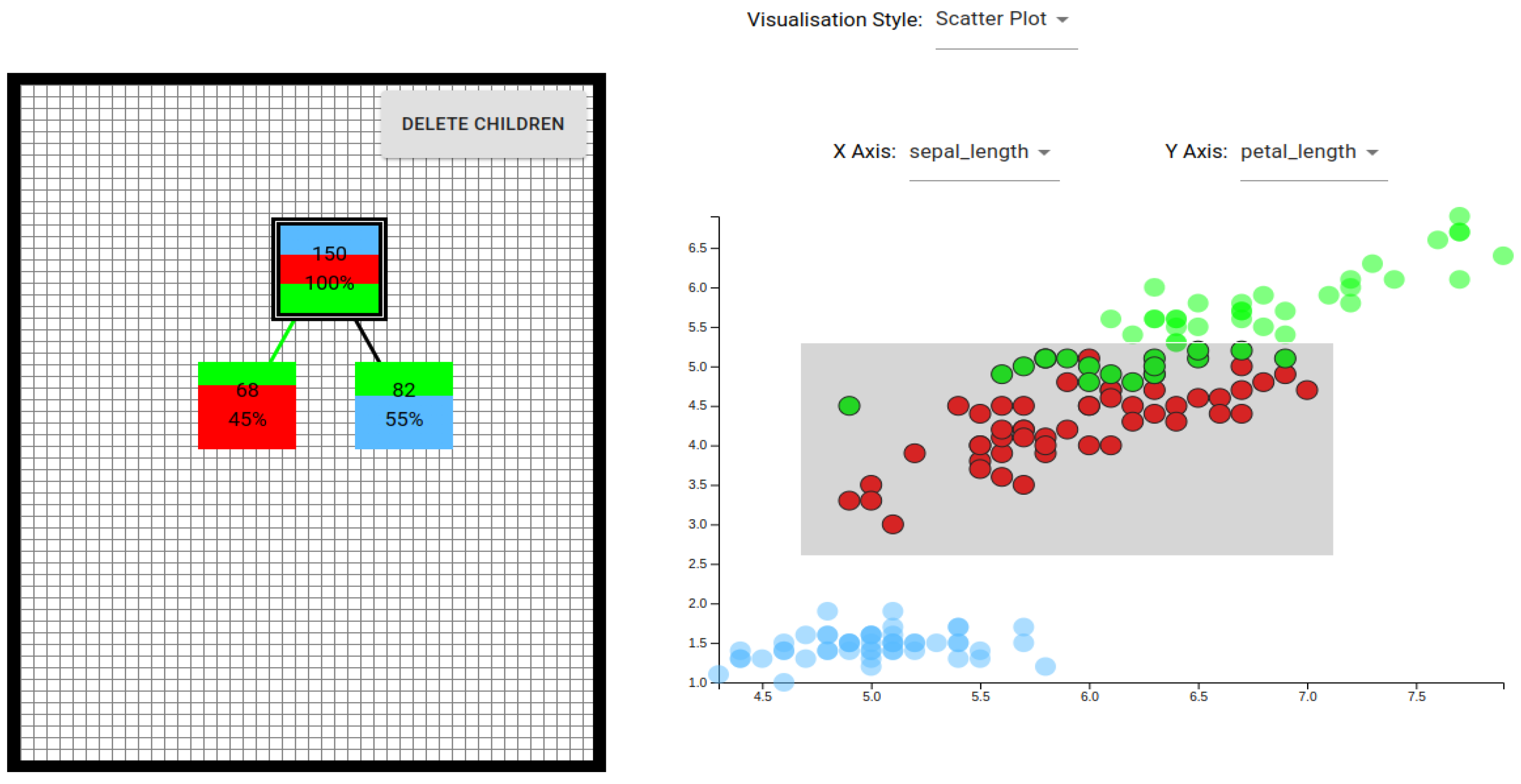
As opposed to the earlier proposals, some empirical evaluation is reported in WEKA’s UserClassifier [14]. UserClassifier is an IML system for DTCs that shows a scatter plot of only two attributes at a time (the user can pivot which two attributes appear in the visualisation). A display of small bars for each attribute provides some assistance for attribute relevance. The attribute bar presents the distribution of classes when sorted by that attribute. The user can review the current tree as a node-link diagram in one display, select, and expand a node. WEKA’s UserClassifier is the only one reporting usability studies, and it involved only five participants [14]. Later, it was evaluated with 50 university students who had completed 7 weeks of material on machine learning and DTCs [45]. This study confirmed a number of limitations of WEKA’s UserClassifier. For instance, the type of interaction (on the dataset and on the model) are restrictive in a number of ways.
  • The visualisation displays only two attributes at a time; this is critically restrictive.
  • The space to display region bars is minuscule, impeding users’ observation of differences to decide which two attributes to display.
  • Despite the immense literature on techniques for splitting a node to grow and construct a decision tree, the system does not provide any split-suggestion to the user.
  • Unless users depart from the attribute visualisation window (losing context of the current splitting task), the tree under construction is not visible.
  • Visualisation techniques (such as colour, or size) are not used. So, the user cannot inspect any properties of a node or an edge nor any relationship between a node and the dataset under analysis.
In summary, these issues limit a human’s ability to gain a broader understanding of the datasets and of the classifiers. Nevertheless, we point out that a comparison of decision trees built by humans against decision trees built by machines resulted in humanly-built trees being superior in many aspects over those built by machines [64]. In that research [64], the technique for human-centred IML was parallel coordinates, which reinforces our approach to include this in our prototype and its evaluation.

3. Iterative Construction of DTCs Supported by Visualisations in Parallel Coordinates

We propose an HITL-ML system that uses parallel coordinates to visualise the training set, the decision tree, and also specific rules. We claim that our proposal addresses key shortcomings of the systems examined in Section 2 including those of the WEKA UserClassifier.

3.1. Using Parallel Coordinates

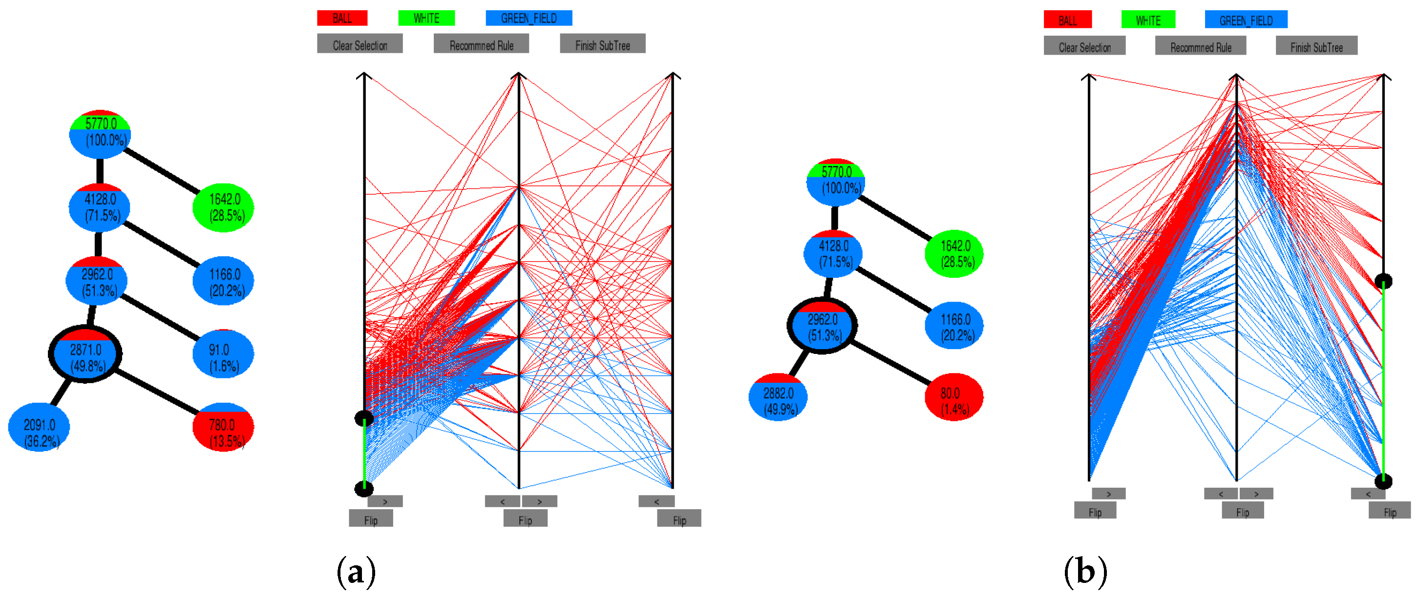
In a parallel-coordinates visualisation, a vertical axis is drawn for each dimension (each attribute). An instance v = ( a 1 , a 2 , , a d ) (a point in Cartesian coordinates) corresponds to a poly-line in parallel coordinates that visits value a n on the axis for attribute A n (for n { 1 , , d } ). For HITL-ML, we assign a different colour to each class, and the labelled instances of the training set are painted using the colour of their label. Figure 1 shows two examples of the parallel coordinate visualisation and the corresponding partially-built decision tree.
If there are many attributes, a window with a projection onto a subset of the attributes is displayed. On-line Analytical Processing (OLAP) tools enable business intelligence practitioners to analyse multidimensional data interactively from multiple perspectives [65]. Our use of colour concentration allows the rapid selection and application of OLAP-type operations on the visible window. For instance, removing one attribute from visualisation and adding another one is a pivot operation. The information gain on an attribute or range within an attribute is used to suggest relevant attributes to the human operator. The visualisation enables domain experts to explore scenarios from their domain knowledge or spot new patterns and hypothesis.
For the specific task of IML, the user will build a DTC following Hunt’s generic recursive construction [43] (p. 152, Chaper 4): the user picks a leaf-node T to further refine the current rule that terminates at T. However, our system provides support for this deeper growth of the tree from leaf T.
  • We colour the corresponding leaf T to illustrate the purity of T (this directly correlates with the classification accuracy of the rule terminating at T). For instance, the left leaf in the tree of Figure 1a indicates it containing an almost even split of two classes. However, the right leaf is practically pure. The depth of the leaf T inversely correlates with the applicability and generality of that rule terminating at T. Understandability and interpretability also inversely correlate with leaf depth.
  • The system allows the user to select whether to display values of predictability power of attributes, such as the information gain.
A tree is always a classifier because the decision at a leaf is the simple Naïve Bayes decision.

3.2. The Splits the User Shall Apply

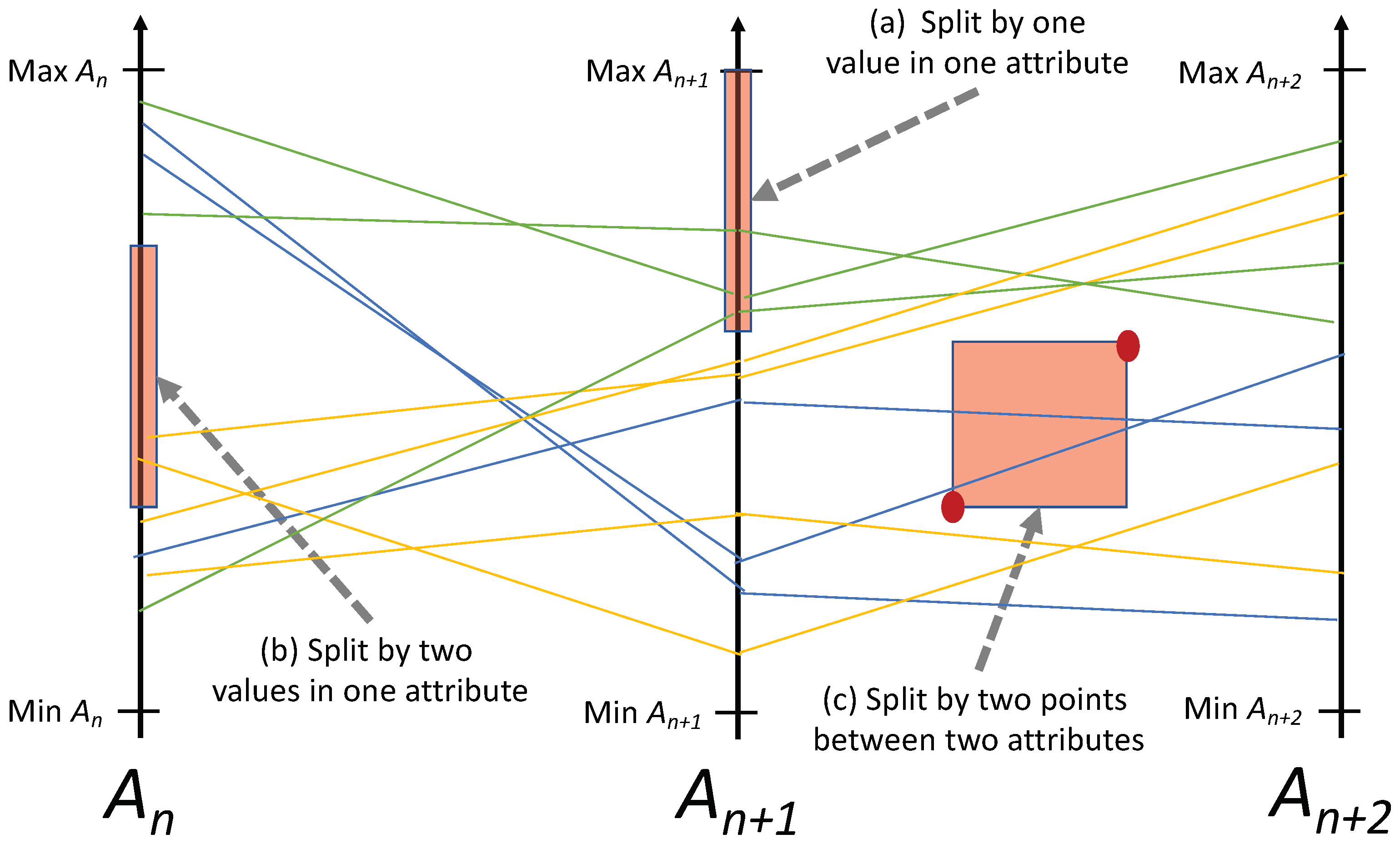
The splits the user can apply were defined in our earlier work [49]. A split on one axis alone is commonly a range, and this is familiar to DTC construction as this is also the type of split evaluated by algorithms such as C4.5 [41] or J48 [66]. However, the parallel-coordinates visualisation allows an oblique split [67,68,69] that involves two attributes. Thus, the oblique test is interpretable particularly because of the point-line duality in parallel coordinates [46]. For instance, a rule that uses a point between two attributes in parallel coordinates means that instances in this split follow two types: first, those that closely follow some linear correlation between two attributes, and second, those that do not reflect such a linear correlation. If we use a rectangular region for the split, then we regulate a margin for the above-mentioned linear correlation. Figure 2 illustrates the types of splits users can introduce in our system.
In addition to the interpretability of the splits based on rectangles between two parallel axes, these splits constitute a richer language to define DTCs than the standard splits of classical machine learning algorithms. Although not as powerful as the full oblique splits [67,68,69], this is appropriate, as full oblique splits are extremely hard to comprehend by humans. DTCs that use oblique splits are also called multivariate decision trees [70,71], and although learning multivariate decision trees results in shorter trees, they are rarely used because the tests (and thus their rules) are incomprehensible by humans.

3.3. Information That Supports Interaction

Our HITL-ML system supports interaction is several ways. For instance, when the user selects a node in the tree, the visualisation restricts the instances displayed in the parallel coordinates’ canvas to those that satisfy the splits of the selected node’s ancestors.
The user can elect several algorithms for ordering attributes in the parallel coordinates’ canvas, which, by default, are sorted by criteria of discriminative power, and among these, the default is information gain. Then, if a user selects an attribute for the next split, the system also offers suggestions for the split on the axis, and again, diverse algorithms are available (again, information gain, gini index, etc.) Moreover, the user can opt for a proposal for a split from the system. Such proposals are rectangular splits computed using evolutionary strategies [49]. The use can accept or modify the rectangle suggested by the system. The automatic construction can be restricted to a node or to a subtree. As the user explores proposed subtrees, the user gains an understanding of the attributes and interaction between attributes. We argue that the algorithms supporting the HITL-ML provide adequate balance between number-crunching and machine learning support, and user’s intervention and interaction to incorporate human expertise, or for users to discover new insights in the data.
We highlight here the crucial role that human pattern spotting has on some of the split selections. For example, Figure 3 represents a setting where humans easily chose better splits than machine learning indicators (such as information gain, gini index). The user can also intervene when machine learning indicators are offering similar values, but some attributes are easier to capture or much more readily available than others.

3.4. Visualising the Tree

As illustrated by the two examples in Figure 1 and those in Figure 4, an interactive display of the tree under construction can be presented on the left of the parallel coordinates’ canvas. As we mentioned, the nodes of the tree are coloured with a histogram that informs the user of the number of instances of each class in the training set that reached the node. We emphasise that this rapidly shows the user the purity (and thus accuracy) of rules reaching a node. The user can also obtain feedback information about the support (percentage of the training set instances that reach the node) and confidence (percent of correct-class classification) for the rule at the node.

3.5. Visualising Rules

So far, we have shown how our HITL-ML system uses parallel coordinates to effectively assist a user in the interactive learning phase of constructing a DTC. We now demonstrate how we can also use parallel coordinates to allow a user to understand a particular classification made by a learnt DTC. Our approach here supports explorative data mining, where experts are seeking to find characteristic rules or discriminant rules [50]. One of the features of DTCs is their ability to be converted into a decision list. Such a decision list is composed of a series of if–else rules that can be followed to determine the classification of a particular instance. We use a similar idea to visualise the decision path for a single leaf in a DTC. Instead of a textual representation of such a rule, however, we can again use parallel coordinates to graphically represent this decision path. We argue that parallel coordinates are ideally suited to this task, as we can use a series of axes to visualise each component of the rule in the one visualisation. Depending on the depth of the rule and available screen real estate, we may even be able to visualise the entire decision path on one screen. Not only this, but in our graphical representation, we can visualise the training data and the effect that each component of the decision path has on the resulting subset of selected data. When used in conjunction with our visualisation of the entire DTC and its accompanying statistics for each node, we argue that this gives a human user a profound, intuitive and interpretable explanation of a DTC’s classification.
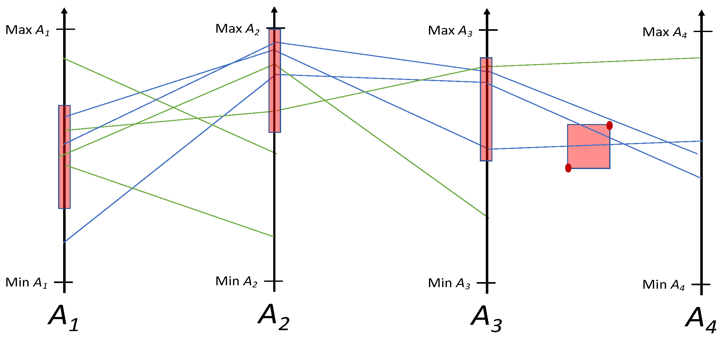
Figure 5 shows an example of how we use parallel coordinates to visualise the decision path to a leaf node in a DTC. Here, the left-most axis is used to represent the split of the root node in the DTC, which will always be the first component in any decision path. In this example, the split for the root node of the decision tree is a simple single attribute split on attribute A 1 and is visualised as such with the highlighted range. Between the first and second axes, the start of poly-lines for every instance in the training set is shown. From the second axis, only instances in the training set continue on that matched the split from the previous axis. This allows the user to easily see what subset of data is selected by each split. The visualisation continues in this manner with poly-lines being terminated once they no longer match a split in the decision path. In this example, the final split in the decision path is a parallel coordinates region split and is visualised using the last two axes.
Another advantage of visualising a particular leaf of a DTC in this way is allowing the user to assess the likelihood that a specific classification is accurate. While traditional performance metrics such as accuracy, ROC, and F1 score capture the performance of the entire tree, it is possible that accuracy varies between individual sections of the model. Using our visualisation, a user can view the amount of the majority class in a leaf node as well as how significant this majority is. When looking at the classification of a particular instance, the user can also see how close to the margins of each split that instance is.

3.5.1. Condensing the Decision Path

In cases where an attribute (or attribute pair in the case of our parallel coordinates region splits) appears more than once in a decision path, we have the opportunity to reduce the number of attributes required to display the decision path by taking the union of both splits. If using only a single attribute split, we can create an upper bound on the number of axes required to visualise any decision path equal to the number of attributes in the dataset. When not condensing the decision path in this way, the ordering of axes in parallel coordinates allows the user to see the depth of each rule in the DTC. For this reason, we provide the user with the option of turning this feature on or off in our HITL-ML system.

3.5.2. Visualising Negated Splits

When visualising a decision path, we need to consider how negated splits are handled. This is important, since half of the sum of all path components are negated splits, i.e., we traverse to the child node that represents the path to take when not matching the node’s split. For single attribute splits of the form l A n , the negated split becomes A n < l and can be represented on a parallel coordinates axis by simply swapping the highlighted region with the region not highlighted. For a single attribute test with two split points of the form l A n r , our negated split becomes A n < l r < A n . This can again be represented on a parallel coordinates axis by swapping the highlighted region with the region not highlighted. Although the representation of this two-value split may seem complicated (particularly, when we consider condensing a decision path that contains the same attributes multiple times), swapping of highlighted regions is simplified using De Morgan Laws [72]. Consider a decision path that includes two components using attribute A n . The first component is of the form l 1 A n r 1 , and the second is the negated form of the split l 2 A n r 2 , i.e., A n < l 2 r 2 < A n . Suppose we have the situation where l 1 < l 2 r 1 > r 2 . In this case, our condensed split becomes l 1 A n l 2 r 2 A n r 1 . To represent this condensed split on a parallel coordinates axis, we now need to highlight multiple disconnected sections of the axis.
Figure 6 illustrates this situation. In a case where the same attribute is used many times in a decision path, the resulting axis consists of several disconnected sections of the axis, which are highlighted (these are disjunctions of intervals). Interestingly, this effect is only possible when using tests containing two split points. Although we have shown in our previous work that using such splits appears to produce less accurate trees, we argue that in an HITL-ML system, it is only natural that a user will want to use these splits containing two split points to isolate certain sections of data, and as such, our system supports the visualisation of condensed rules of this form.

4. Materials and Methods

We now report on the design, materials and methods for a comprehensive study evaluating our prototype. We obtain quantitative data on the effectiveness of our visualisation techniques from an online survey using the custom built survey platform Prolific [73]. The quantitative data are from 104 participants who performed timed tasks using variants of our new visualisation techniques and HITL-ML approach, resulting in 8944 data points.
Our survey starts by reviewing three concepts applicable to HITL-ML. These three concepts are (1) DTC (2) PC, and (3) scatter-plot based visualisation techniques. This refresher practice ensures we can rank the expertise with ML topics of our participants and exclude any not fluent with DTC construction. Then, the survey requires users to complete tasks building DTC on a platform for automatic data collection [73]. In addition to the facility to animate aspects of the visualisations, the online platform allowed us to select participants who had experience in ML.

4.1. Recruiting Participants

Research studies using Prolific [73] commonly use the capability to enable participation to only specific demographics. We also selected participants whose answers to demographic questions were as follows.
  • Which of the following best describes the sector you primarily work in? Information Technology, Science, Technology, Engineering and Mathematics;
  • What is your first language? English;
  • Which of these is the highest level of education you have completed? Undergraduate degree (BA/BSc/other);
  • Do you have computer programming skills? Yes/No.

4.2. Survey Design

The online survey consists of three different experiments and offers participants user interaction as if they were performing tasks in a system for HITL-ML. Not only does the system display videos and allow users to click on images to experiment, while moving forward and back through explanations, it also enables interactivity in all components when building DTC, including display, the selection of nodes, and their expansion. In addition, the system allows users to configure some parameters of these visualisations.
The first experiment examines the effectiveness of visualising a DTC using a node-link diagram with coloured nodes (see Figure 1). The second experiment examines participants’ ability to understand the classification of individual instances, comparing the traditional method of traversal of a DTC against the PC-based visualisation of the path to a leaf node. In the third experiment, pairs of videos are played to the participants, contrasting two different HITL-ML systems. Showing videos removes the participants’ need to gain sufficient expertise with GUI aspects that are not the core of the visualisation. Nevertheless, participants can evaluate how well a system supports the user to perform a HITL-ML task.
Before starting the survey, each participant is randomly placed in one of two evenly sized groups (Group A and Group B). Participants from each group are shown slightly different visualisations when completing tasks in Experiment 1 and Experiment 2 with the aim of evaluating what effect these visualisations have on a participant’s ability to complete the tasks in each experiment. This also requires that the sections introducing participants to visualisation techniques be presented and ordered slightly differently. The arrows in Figure 7 show the sections displayed to each group in the order (work-flow) from the perspective of participants. We now detail the exact composition of each experiment and the introductory section of the survey.

4.2.1. Experiment 1—DTC Node Colouring

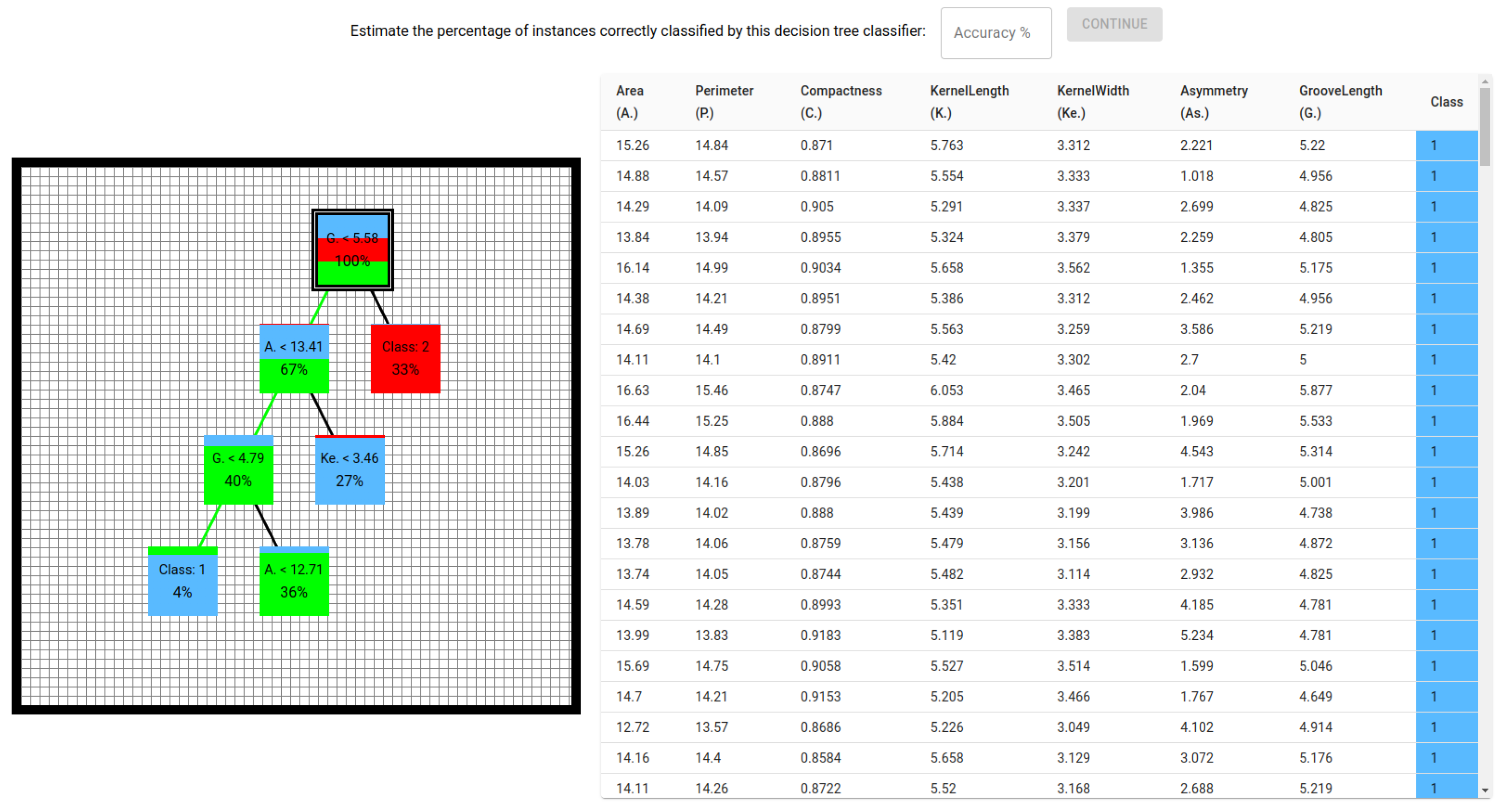
Experiment 1 examines the effect that colouring the nodes of a DTC has on a participant’s ability to interpret the tree. Specifically, this experiment looks at the ability to use a visualisation of a DTC to estimate the accuracy of the entire tree as well as subsections thereof. Participants are shown several different DTC and are required to complete two tasks for each DTC. The first task requires participants to estimate the accuracy of the DTC. Then, participants must select a single leaf node that they believe ‘is most in need of further refinement to improve the accuracy of the classifier’. Figure 8 shows the layout of this experiment. The objective of these tasks is to provide evidence for the following hypotheses.
Hypothesis 1.
The technique of colouring nodes will allow a user to more accurately estimate the predictive power of a DTC.
Hypothesis 2.
The technique of colouring nodes will allow a user to more quickly estimate the predictive power of a DTC.
Hypothesis 3.
The technique of colouring nodes will allow a user to more accurately identify the most impure nodes in a DTC.
Hypothesis 4.
The technique of colouring nodes will allow a user to more quickly identify the most impure nodes in a DTC.
On the left of the screen, the system presents a visualisation of a DTC to both groups of participants (there is no difference in this aspect for Group A and Group B). The right half of the screen shows a table containing the training data used to learn the DTC. This table also has a colour coding for the class column for both Group A and Group B. For participants in Group B, the nodes of the DTC are also coloured. For each tree, participants are first asked to estimate the accuracy of the tree by entering an integer between 0 and 100. Using accuracy rather than the F-measure ensured that all participants were familiar with the statistic used. Given that accuracy is a much simpler statistic to calculate than F-measure, asking for accuracy also ensures that the cognitive load on the participant is reduced as much as possible.
After estimating the accuracy of each DTC, participants are asked to select the leaf node they ‘believe is most in need of further refinement to improve the accuracy of the classifier’. To quantify the accuracy of a user’s choice, we use a metric R I m p ( n ) , describing the impurity of a node in a DTC relative to the most impure node in the tree. Let n be defined as a leaf node in a DTC containing N leaf nodes. Furthermore, let I ( n ) be the number of instances of training data that reach n, whose class is not the majority class of instances reaching n.
Definition 1.
We can then define I m a x ( N ) as follows:
I m a x ( N ) = max { I ( n ) n N } .
The following now defines our evaluation metric.
Definition 2.
We define R I m p ( n ) , the relative impurity of a node, as
R I m p ( n ) = ( I m a x ( N ) I ( n ) ) I m a x ( N ) .
Each participant is shown eight different DTCs that were constructed from three datasets. We use three datasets available from the UCI-repository [74], the Wine (Available online: https://archive.ics.uci.edu/ml/datasets/Wine, accessed on 3 April 2020), Cryotherapy (Available online: https://archive.ics.uci.edu/ml/datasets/Cryotherapy+Dataset+, accessed on 3 April 2020) and Seeds (Available online: https://archive.ics.uci.edu/ml/datasets/seeds, accessed on 3 April 2020) datasets. These three datasets exhibit the following relevant properties.
  • A reasonably accurate (>90% accuracy) DTC can be learnt for each dataset with small trees sizes that remain interpretable to a human.
  • All attributes have humanly understandable names and semantic meaning.
Using these three datasets, eight DTCs were built with a range of different accuracies for two reasons. First, having different accuracies for each DTC ensures that there are no patterns in the survey that participants can use to help them assess the accuracy of any individual tree. Second, having a range of accuracies ensures that participants’ ability to assess the accuracy of a DTC is not dependent on the DTC having a particularly low or high accuracy. Table 1 shows the true accuracy of each DTC presented to participants. For each participant, we record the following information.
  • Their prediction of the accuracy of each DTC.
  • The time taken to predict the accuracy of each DTC.
  • The leaf node selected by the participant as most impure for each DTC.
  • The time taken to select the most impure leaf node in each DTC.

4.2.2. Experiment 2—Rule Visualisation

This experiment evaluates the effectiveness of representing the path from a root node to a leaf node using PC. Figure 9 shows the layout of this experiment. For this experiment, participants must determine whether a given instance reaches a particular leaf node in a DTC. Participants in Group A and Group B are shown two different visualisations while performing this task. For participants in Group A, this visualisation consists of a DTC on the left half of the screen and a table on the right half of the screen. The DTC on the left is represented as a simple node-link diagram with the split criteria for each internal node represented textually within the node. As part of this visualisation, a green arrow points to one of the nodes in the DTC. The table on the right contains a single row with the attribute values of one instance. Group A participants are required to manually traverse the DTC for the instance shown in the table and determine whether it arrives at the node indicated by the green arrow. Group A participants are also shown a table with a single instance containing the attribute values to be used to traverse the tree.
Group B participants are shown a PC visualisation of the path to a particular leaf node in a DTC. This PC visualisation shows the entire dataset as well as ranges on several of the PC axes to represent each of the univariate splits on the path to the leaf node. The polyline for one of the instances is shown as a distinct thick black line. Group B participants are required to determine if this instance arrives at the leaf node being visualised using PC.
Participants in both groups use the same set of instances and DTC. The DTCs used are the same as those in Experiment 1. For each DTC, participants must evaluate three instances from the dataset used to create the DTC. Participants answer whether they think this instance reaches the selected leaf node. This experiment tests the following hypotheses.
Hypothesis 5.
Participants visualising the path to a node using PC will more accurately determine whether an instance reaches a particular leaf node.
Hypothesis 6.
Participants visualising the path to a node using PC will more quickly determine whether an instance reaches a particular leaf node.

4.2.3. Experiment 3—Human-in-the-Loop Video Survey

This experiment evaluates several HITL-ML features proposed earlier. For each pair of videos, one video illustrates a particular HITL-ML task being performed using a system based on the techniques proposed earlier. The other video in each pair shows how the same task is carried out using Weka’s UserClassifier. After viewing both videos, participants are required to express their preference on a five-point Likert scale. At the start of the experiment, the survey system randomly decides which HITL-ML system’s video will be shown to each participant first. The order then remains the same for all video pairs for this participant. In total, five different pairs of videos demonstrate a variety of HITL-ML tasks. A description of each video pair and its questions are given below. Table 2 also shows a summary of the questions asked for each video pair. After answering the Likert-scale questions for each of the five pairs of videos, the survey system asks participants one final Likert scale question. This question asks participants, ‘Based on the videos you’ve seen, which system would you prefer to use to build a decision tree classifier?’
The tasks on the activities with videos are as follows.
  • The first pair of videos examines the ability of a user to find an effective split for a node in a DTC. In the UserClassifier video, survey participants are shown how the dataset is visualised using a two-dimensional scatter-plot as well as how a user can select attributes using the small bar visualisation of each attribute on the right of the screen. The video then demonstrates how a user can construct a split for a node by selecting a region on the two-dimensional scatter-plot. The PC-based video shows how a dataset is visualised using PC and how a user can create a split by selecting a range on an axis. This video also shows how a user can rearrange axes and remove axes that are not of interest. In addition, participants are shown how a user can ask the PC-based system to reorder axes so that interesting axes appear on the far left. This rearrangement is achieved by ordering axes based on the best gain ratio of each attribute, as discussed in Section 3.3. At the end of both videos, participants are asked, ‘Which system do you believe provides a better method of finding splits to build a decision tree classifier?’
  • The next pair of videos examines a user’s ability to navigate and understand a DTC in each HITL-ML system. The UserClassifier video shows how a user can switch to a separate tab from the training set visualisation to observe the current state of the DTC being constructed. Participants are shown how internal and leaf nodes are displayed as grey circles and rectangles, respectively. This video also shows how splits for each internal node can be observed by selecting the node and switching tabs to see the selected region in the dataset visualisation tab. The PC-based video demonstrates how the system splits one window into two sections. The video shows how the left section visualises the DTC using the coloured nodes. This video also demonstrates how a user can interact with this DTC and select a node, at which point any split for that node is shown on the far left axis in PC. After viewing both videos, the survey system asks participants, ‘Which system allows you to better navigate and understand the current state of a decision tree classifier as it is being constructed?’
  • The third set of videos looks at a user’s ability to estimate the accuracy of a DTC using each HITL-ML system. The UserClassifier video shows participants how a user can look at the counts of instances shown in each leaf node to determine the majority class and how often this leaf misclassified training instances. This video also demonstrates how a user can assess the quality of a split for a node by visualising it with the training set in the second tab of the system. The PC-based video shows participants how a user can use the colouring of the nodes in the DTC to determine the accuracy of each leaf node. Participants are also shown how a user can assess the quality of a split using the visualisation of the split in PC. After both videos, participants are asked, ‘Which system allows you to more easily determine how often a tree will predict the correct class of an instance?’
  • The fourth pair of videos examines the ability of a user to locate nodes in a DTC that requires further refinement. In the UserClassifier video, participants are shown how a user can use the visualisation of the DTC and the numbers within each node to find leaf nodes with a large number of instances from multiple classes. The PC-based video shows participants how a user can use the colouring of nodes to determine which nodes require further refinement. Following these videos, participants are asked, ‘Which system allows you to more easily find nodes in a decision tree classifier that need additional splits?’
  • The final pair of videos look at the algorithmic assistance features offered by each system. In the UserClassifier video, participants are shown how a user can use an automated algorithm to complete a subtree. This video points out to participants that the user has no way of visualising the generated subtree or determining any of its characteristics. The PC-based video shows how a user can ask the system to suggest a test for a node in the tree and how this test can be visualised for the user. This video also shows how the system can complete a subtree for the user, which can be visualised and edited as deemed appropriate by the user. Following these videos, participants are asked, ‘Which system would provide better assistance to you when constructing a decision tree?’

4.3. Methods

4.3.1. Introduction to Decision Trees

As we explained, the first section of the survey provides users with an introduction to DTCs. This introduction is structured as a review that illustrates all examples with the Iris dataset. Figure 10 shows the layout of the user’s window on the survey. Subjects are first presented with a scrollable table containing the complete Iris dataset. Using interactive prompts, the survey introduces participants to terminology, such as an instance in a dataset, what the class of an instance is, and the goals of a classification task.
After the introduction to the basic terminology about datasets, participants are introduced to DTCs. Subjects work through an interactive visualisation of a DTC for the Iris dataset. This DTC visualisation is similar to the node-link visualisation of a DTC described in Section 3.4. The participant is able to click on each node in the tree to filter the instances displayed in the tables of the Iris dataset. Interactive prompts guide the participants through the following concepts.
  • The structure of a DTC.
  • How to evaluate univariate splits on internal nodes in a DTC.
  • How to traverse a DTC.
  • How a DTC can be used to classify an instance.
  • How the class label assigned to a leaf node is determined via the majority class of instances reaching that leaf.
  • Examples of a DTC incorrectly classifying instances.
  • How a user might use the presented visualisation of a DTC to estimate its accuracy.
Participants in Group B are additionally introduced to the concept of colouring nodes in the visualisation of the DTC in this section. This is the visualisation technique introduced in Section 3.4, where each node in the DTC is coloured such that the amount of each colour in a node is proportionate to the amount of the corresponding class reaching the node.
Before moving to the next section in the survey, participants from Group A and Group B are shown how they can estimate the accuracy of a DTC by looking at the impurity of each leaf node. Participants from Group B are also shown how the colouring of nodes can help in this process.

4.3.2. Introduction to Parallel Coordinates

In this section, participants are given an introduction to PC. Similar to the first section of the survey, participants are shown a table containing the Iris dataset. Next to this table, users are shown a parallel coordinates representation of the Iris dataset. Figure 11 shows the layout of this section of the survey. We designed the survey system to require participants to click through several interactive prompts, highlighting the following features.
  • How each instance is represented in parallel coordinates.
  • The use of colour in each poly-line to indicate the class of an instance.
  • The ability for a user to toggle a numerical scale for all axes on and off.
  • Coloured buttons at the top of the PC visualisation which allow a user to show/hide individual classes.
To increase a participant’s understanding of PC, an additional visualisation technique is included in this section. Participants are able to hover their mouse over an individual instance in the table of the Iris dataset. When a participant hovers their mouse over an instance, the corresponding polyline for the instance in PC is emphasised using a bold black colour. Participants are encouraged to explore how individual instances in the Iris dataset are mapped to the PC visualisation before moving to the next section.

4.3.3. Decision Tree Classifiers with Parallel Coordinates

This section shows participants how PC and the DTC visualisation introduced in the previous sections can be combined into one system. This visualisation presented to participants is similar to the HITL-ML system introduced in Section 3.1, with the left half of the screen displaying the DTC and the right half of the screen visualising a dataset with PC. The Iris dataset is used again to introduce participants to this system. Participants are introduced to the following features of the combined visualisation.
  • How selecting a node in the DTC filters the instances shown in PC.
  • How univariate splits can be represented in PC as a range on an axis.
For participants in Group B, this section is also used to introduce the technique of using PC to visualise all splits in the path from the root node to a particular leaf node in a DTC. This is the visualisation technique introduced in Section 3.5. Group B participants are shown the following features of this visualisation technique.
  • How the poly-lines for all instances in this visualisation originate from an origin point before passing through each axis in PC.
  • How all splits in the path to a leaf node are shown as a series of ranges on PC axes.
  • How axes are ordered to match the order of attributes appearing in the path to the leaf node.
  • How the poly-line for each instance is terminated when it does not match the range on a PC axis.
  • How each poly-line is dimmed after it passes through all required ranges to reach a leaf node.
This section of the survey appears directly before Experiment 2 for participants in Group B. In Experiment 2, Group B participants are required to use the PC visualisation of the path to a leaf node to determine if an instance reaches a particular leaf. This section explains to Group B participants the structure of questions in Experiment 2 and how to use the visualisation techniques introduced to complete Experiment 2.
For participants in Group A, this section introduces the node colouring technique that was shown previously (in the first section) to participants in Group B. This node colouring technique is shown here for participants in Group A to ensure that they have been introduced to all the same visualisation techniques as those in Group B before the start of the last section on HITL-ML. The only exception to this is the use of PC to visualise the path to a leaf node. Participants from Group A are not shown this visualisation technique, since it has no relevance to any of the content in the HITL-ML section of the survey.

4.3.4. Evaluating Decision Tree Classifiers

This section of the survey appears only for participants in Group A. It aims to prepare Group A participants for Experiment 2, where they will be asked to determine if a given instance reaches a particular leaf node in a DTC. No new visualisation techniques are introduced in this section. Instead, Group A participants are shown two examples of how to traverse a DTC for a given instance. Participants are shown a table with a single instance. An interactive tutorial guides participants through the traversal of a DTC for each instance. This tutorial shows participants an example of a situation where an instance does or does not reach a particular leaf node and how to answer questions of this nature.

4.3.5. Human-in-the-Loop-Learning of Decision Tree Classifiers

In this section of the survey, participants are given an introduction to the concepts behind HITL-ML. Figure 12 shows the layout of this survey section. The Iris dataset is again used to introduce these concepts. The section begins with several interactive prompts explaining how a user can build a DTC using HITL-ML. Participants are then encouraged to use a simplified HITL-ML system to create a DTC for the Iris dataset. This aims to ensure users understand the concepts behind HITL-ML, before providing feedback on the two HITL-ML systems presented in Experiment 3. To minimise bias towards one visualisation style, the HITL-ML system in this section allows a participant to select their preferred visualisation style to build a DTC using a two-dimensional scatter-plot and PC.

5. Results

5.1. Experiment 1

A total of 51 participants from Group A and 53 participants from Group B completed this experiment. Table 3 shows the average results for each group. From this table, we can see that when estimating the accuracy of a DTC, participants in Group B appear to be slightly less accurate than those in Group A, but they managed to make their estimation much faster. Similarly, when selecting the most impure leaf in a DTC, the mean relative impurity of leaf nodes selected by participants in Group B was slightly higher; however, the time to choose this leaf node was quicker than participants in Group A.
We now proceed to evaluate as to whether the results accounted for statistically significant differences in the results between Groups A and B. Since some of the results obtained in this experiment are not normally distributed as determined by the Shapiro–Wilk test [75], we use the Wilcoxon–Mann–Whitney test to check for statistically significant differences between Group A and Group B as opposed to a t-Test. The Wilcoxon–Mann–Whitney test is a nonparametric equivalent to the t-Test to compare independent samples [76]. Performing this statistical test on the accuracy differences and R I m p results in p-values of 0.196 and 0.311 , respectively. As such, we cannot reject the null hypotheses that Group A and Group B perform equally in terms of ability to estimate the accuracy of a DTC and ability to find the most impure nodes in a DTC and must reject Hypotheses 1 and 3. Performing statistical tests on accuracy time and leaf selection time results in p-values of 3.65 × 10 10 and 0.006 , respectively. Here, the differences in time for both tasks in this experiment are statistically significant. As such, we can accept Hypotheses 2 and 4. Although this experiment showed that colouring nodes does assist users to more quickly assess the predictive power of a DTC and find leaf nodes requiring further refinement, node colouring appears to have minimal impact on how accurately participants perform these tasks.

5.2. Experiment 2

Like Experiment 1, Experiment 2 consisted of 51 participants in Group A and 53 participants in Group B. For each participant, we calculate the percentage of questions where the participant provided the correct answer. Table 4 shows the average result from Group A and Group B for Experiment 2. These average accuracies show clear differences in the performance between the two groups. Using the PC-based visualisation, participants in Group B answered 86.7% of questions correctly. This is in contrast to Group A participants, who only achieved 77.5% accuracy. Group B participants also appear to be able to determine whether an instance reaches a leaf node faster than Group A participants. On average, Group B participants only required approximately one-quarter of the time to determine whether an instance reached a leaf as those in Group A. Using the Wilcoxon–Mann–Whitney Test, we confirm that the average accuracy and time results are statistically significant with p-values of 1.51 × 10 9 and < 2.2 × 10 16 , respectively. As such, Hypotheses 5 and 6 are accepted. We argue these results demonstrate a clear advantage to the use of PC to allow humans to interpret DTC. Using PC dramatically decreased the mistakes made when interpreting the splits for a DTC as well as allowing participants to more quickly interpret the series of splits leading to the classification of an instance.

5.3. Experiment 3

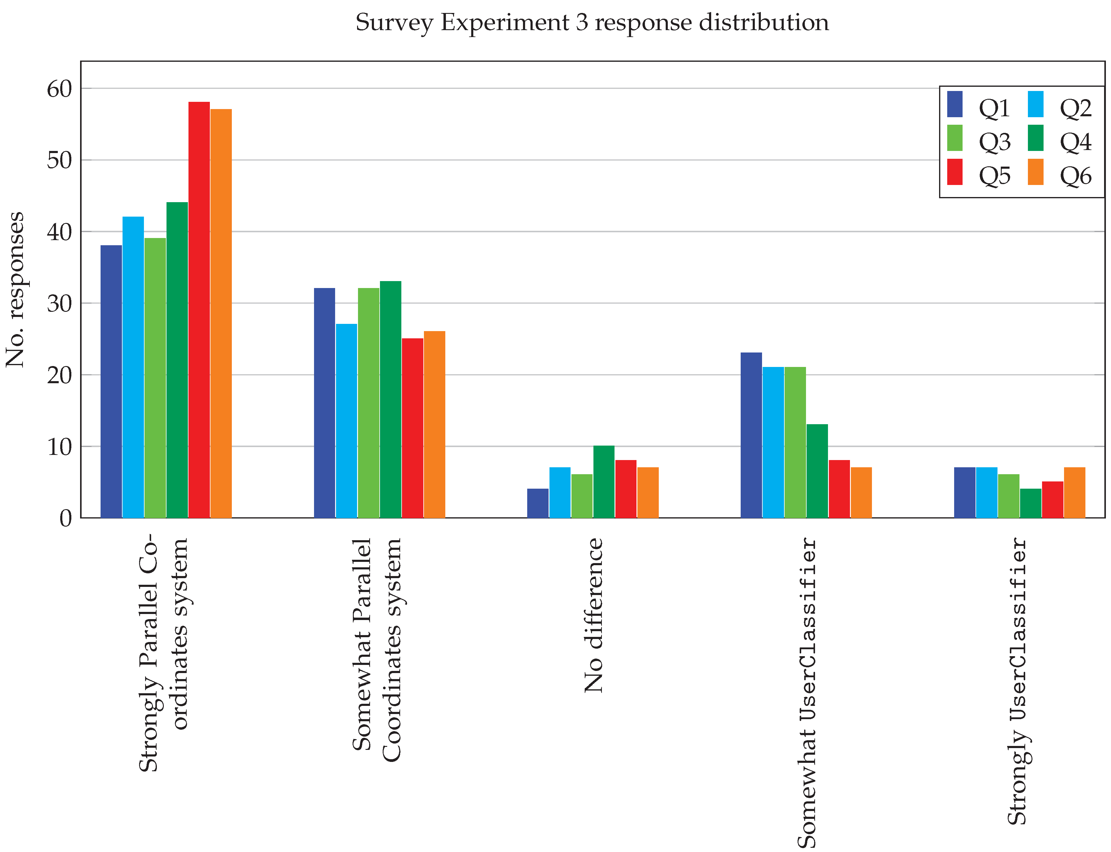
Experiment 3 was completed by 104 participants. Table 5 shows a summary of the responses received for each question in the experiment. Figure 13 also visualises the distribution of responses received for each question. We can see from these results that there is a clear preference for the PC-based system for all HITL-ML tasks examined. For each of the five pairs of videos, between 66.3% and 79.8% of participants had some preference for the PC-based system. In addition, participant responses from the last question showed 79.8% of participants had an overall preference for the PC-based system.

5.4. Validity Threats

We now discuss the internal and external validity of the results obtained from the experiments in this section. We note three possible threats to the internal validity of these experiments. First, as this survey was conducted online, participants could not be observed as they carried out these experiments. In both Experiment 1 and Experiment 2, the survey system records the time taken for participants to complete each task. These time measurements could be affected by participants taking breaks or being distracted while completing the survey. Second, we designed the interactive tutorials in this survey under the assumption that participants had limited experience with PC. Some intuition often needs to be built when using PC. Participants that did have previous experience using PC may have performed better on certain tasks in these experiments than participants that had no or limited experience using PC. Finally, we note that all participants completed this survey using their own computers. Given the importance of available screen real estate for any data visualisation, the size of the monitor a participant used may have affected their performance. While we made every effort to ensure that the survey system works well on a variety of screen sizes, participants with larger monitors may have found some visualisations presented in this survey easier to interpret.
Regarding external validity for this survey, we note that participation in the survey was restricted to participants with a bachelor’s level education who are working in the STEM field. Participants with a higher level of expertise in ML or data visualisation may have found the visualisation techniques presented in this survey more intuitive to use and performed better at the tasks included in this survey.

6. Discussion

Many have argued that there are clear advantages of human-in-the-loop for machine learning tasks [12,14,17,19,60,61,77]. In particular, the structural breakdown of an IML system highlights that through the interface, the users not only interact with the data but also interact with and conceptualise the model [47], which goes far beyond what an after-the-fact interpretation of a black-box machine learning classification can achieve. We have explored here the effectiveness of our proposed interface for both of these aspects. Our prototype uses parallel coordinates to visualise and interact with the data, scaling into high levels of dimensionality while retaining the ability to re-order and focus on important attributes. Crucially, our proposal also delivers the modes of interaction with the model (the classifier) that are necessary for constructive conceptualisation. The oblique tests in particular are components of the model that directly benefit from the parallel coordinates layout and its ability to make an otherwise highly dimensional attribute space, that transcends human comprehension, accessible through re-ordering and focussing on individual as well as adjacent dimensions. These aspects are essential for the close interaction expected of IML, where users and learning systems are coupled by focussed and frequent interactions [18]. Our prototype and our analysis advances the crucial element in IML of how the model can be frequently and incrementally updated [48,78].
Our approach here shows how effective visualisation can involve a human expert in expeditiously guiding the construction of interpretable classification models. Moreover, our IML system not only contributes to explainable AI by producing conceptually understandable models; it also allows a user to revise the objective of classification accuracy when alternatives manifest themselves as important objectives. Furthermore, we have proposed how to visualise and elaborate on characterisation and discrimination rules where users are interested in one class above the others. We have also emphasised that while decision trees rank highly overall as a model for HITL-ML classification, by reordering attributes based on the importance perceived through our visualisation, we can strike a suitable balance between multi-variate decision tress and uni-variate decision trees. Users can propose bi-variate splits they visually discover between adjacent attribute axes, that remain understandable, even in high overall dimensionality, in our parallel coordinates canvas.
In the literature, IML has hardly been evaluated with human participants [52]. This paper also provides a large study and suggests a methodology for evaluation. As such, the experiments described here not only support our claims regarding the interface but constitute a model and a benchmark for the assessment of IML.

Author Contributions

Conceptualisation, V.E.-C., E.G. and R.H.; methodology, V.E.-C., E.G. and R.H.; software, E.G.; validation, V.E.-C., E.G. and R.H.; analysis, E.G.; investigation, V.E.-C., E.G. and R.H.; resources, E.G.; data curation, E.G.; writing—original draft preparation, V.E.-C. and R.H.; writing—review and editing, V.E.-C., E.G. and R.H.; visualisation, E.G.; supervision, V.E.-C. and R.H. All authors have read and agreed to the published version of the manuscript.

Funding

This research received no external funding.

Institutional Review Board Statement

The study was conducted in accordance with the Declaration of Helsinki, and approved by the Ethics Committee of Griffith University (protocol code 2021/538, March 2021) for studies involving humans.

Informed Consent Statement

Informed consent was obtained from all subjects involved in the study.

Data Availability Statement

The data presented in this study are openly available in https://github.com/eugene-gilmore/dtc-survey-results (accessed on 3 April 2020).

Acknowledgments

Eugene Gilmore is thankful to the Griffith Graduate Research School (Griffith University) for support during some of his PhD program through a Higher Degree Research Scholarship (Australian Postgraduate Award). All authors are thankful for the support of the School of ICT (Griffith University) that funded the cost of the survey in the survey platform Prolific [73].

Conflicts of Interest

The authors declare no conflict of interest.

Abbreviations

The following abbreviations are used in this manuscript:
CARTClassification and Regression Trees
DTCDecision Tree Classifier
XAIExplainable Artificial Intelligence
HITL-MLHuman-In-The-Loop Machine Learning
IMLInteractive Machine Learning
MLMachine Learning
NCNested Cavities Algorithm
PCParallel Coordinates

References

  1. Dzindolet, M.T.; Peterson, S.A.; Pomranky, R.A.; Pierce, L.G.; Beck, H.P. The role of trust in automation reliance. Int. J. Hum.-Comput. Stud. 2003, 58, 697–718. [Google Scholar] [CrossRef]
  2. Darlington, K. Aspects of Intelligent Systems Explanation. Univers. J. Control. Autom. 2013, 1, 40–51. [Google Scholar] [CrossRef]
  3. Dominguez-Jimenez, C. PROSE: An Architecture for Explanation in Expert Systems. In Proceedings of the Third COGNITIVA Symposium on at the Crossroads of Artificial Intelligence, Cognitive Science, and Neuroscience, COGNITIVA 90, Madrid, Spain, 20–23 November 1990; North-Holland Publishing Co.: Amsterdam, The Netherlands, 1991; pp. 305–312. [Google Scholar]
  4. Swartout, W.R.; Moore, J.D. Explanation in Second Generation Expert Systems. In Second Generation Expert Systems; David, J.M., Krivine, J.P., Simmons, R., Eds.; Springer: Berlin/Heidelberg, Germany, 1993; pp. 543–585. [Google Scholar]
  5. Ye, R.L.; Johnson, P.E. The Impact of Explanation Facilities on User Acceptance of Expert Systems Advice. MIS Q. 1995, 19, 157–172. [Google Scholar] [CrossRef]
  6. Wang, N.; Pynadath, D.V.; Hill, S.G. Trust calibration within a human-robot team: Comparing automatically generated explanations. In Proceedings of the 2016 11th ACM/IEEE International Conference on Human-Robot Interaction (HRI), Christchurch, New Zealand, 7–10 March 2016; pp. 109–116. [Google Scholar] [CrossRef]
  7. Machlev, R.; Perl, M.; Belikov, J.; Levy, K.Y.; Levron, Y. Measuring Explainability and Trustworthiness of Power Quality Disturbances Classifiers Using XAI—Explainable Artificial Intelligence. IEEE Trans. Ind. Inform. 2022, 18, 5127–5137. [Google Scholar] [CrossRef]
  8. Weiss, S.M.; Kulikowski, C.A. Computer Systems That Learn: Classification and Prediction Methods from Statistics, Neural Nets, Machine Learning, and Expert Systems; Morgan Kaufmann Publishers Inc.: San Francisco, CA, USA, 1991. [Google Scholar]
  9. Quinlan, J.R. Induction of Decision Trees. Mach. Learn. 1986, 1, 81–106. [Google Scholar] [CrossRef]
  10. Henery, R.J. Chapter 2: Classification. In Machine Learning, Neural and Statistical Classification; Michie, D., Spiegelhalter, D.J., Taylor, C.C., Eds.; Ellis Horwood: New York, NY, USA, 1995; pp. 6–16. [Google Scholar]
  11. Kodratoff, Y. Chapter 8: Machine Learning. In Knowledge Engineering Volume I Fundamentals; Adeli, H., Ed.; McGraw-Hill, Inc.: New York, NY, USA, 1990; pp. 226–255. [Google Scholar]
  12. Ankerst, M.; Elsen, C.; Ester, M.; Kriegel, H.P. Visual Classification: An Interactive Approach to Decision Tree Construction. In Proceedings of the Fifth ACM SIGKDD International Conference on Knowledge Discovery and Data Mining, KDD’99, San Diego, CA, USA, 15–18 August 1999; ACM: New York, NY, USA, 1999; pp. 392–396. [Google Scholar] [CrossRef]
  13. Estivill-Castro, V. Collaborative Knowledge Acquisition with a Genetic Algorithm. In Proceedings of the 9th International Conference on Tools with Artificial Intelligence, ICTAI’97, Newport Beach, CA, USA, 3–8 November 1997; IEEE Computer Society: Newport Beach, CA, USA, 1997; pp. 270–277. [Google Scholar] [CrossRef]
  14. Ware, M.; Frank, E.; Holmes, G.; Hall, M.; Witten, I.H. Interactive machine learning: Letting users build classifiers. Int. J. Hum.-Comput. Stud. 2001, 55, 281–292. [Google Scholar] [CrossRef]
  15. Webb, G.I. Integrating machine learning with knowledge acquisition through direct interaction with domain experts. Knowl.-Based Syst. 1996, 9, 253–266. [Google Scholar] [CrossRef] [Green Version]
  16. Sacha, D.; Kraus, M.; Keim, D.A.; Chen, M. VIS4ML: An Ontology for Visual Analytics Assisted Machine Learning. IEEE Trans. Vis. Comput. Graph. 2019, 25, 385–395. [Google Scholar] [CrossRef]
  17. Amershi, S.; Cakmak, M.; Knox, W.B.; Kulesza, T. Power to the People: The Role of Humans in Interactive Machine Learning. AI Mag. 2014, 35, 105–120. [Google Scholar] [CrossRef]
  18. Mosqueira-Rey, E.; Hernández-Pereira, E.; Alonso-Ríos, D.; Bobes-Bascarán, J.; Fernández-Leal, A. Human-in-the-loop machine learning: A state of the art. Artif. Intell. Rev. 2022, 35, 1–19. [Google Scholar] [CrossRef]
  19. Fails, J.A.; Olsen, D.R. Interactive Machine Learning. In Proceedings of the 8th International Conference on Intelligent User Interfaces, IUI’03, Miami, FL, USA, 12–15 January 2003; Association for Computing Machinery: New York, NY, USA, 2003; pp. 39–45. [Google Scholar] [CrossRef]
  20. Krak, I.; Barmak, O.; Manziuk, E.; Kudin, H. Approach to Piecewise-Linear Classification in a Multi-dimensional Space of Features Based on Plane Visualization. In Advances in Intelligent Systems and Computing, Proceedings of the International Scientific Conference “Intellectual Systems of Decision Making and Problem of Computational Intelligence”, Kherson, Ukraine, 25–29 May 2020; Lytvynenko, V., Babichev, S., Wójcik, W., Vynokurova, O., Vyshemyrskaya, S., Radetskaya, S., Eds.; Springer International Publishing: Cham, Switzerland, 2020; pp. 35–47. [Google Scholar] [CrossRef]
  21. Freitas, A.A. Comprehensible classification models: A position paper. SIGKDD Explor. 2013, 15, 1–10. [Google Scholar] [CrossRef]
  22. Guidotti, R.; Monreale, A.; Ruggieri, S.; Turini, F.; Giannotti, F.; Pedreschi, D. A survey of methods for explaining black box models. ACM Comput. Surv. (CSUR) 2018, 51, 1–42. [Google Scholar] [CrossRef]
  23. Lavrač, N. Selected techniques for data mining in medicine. Artif. Intell. Med. 1999, 16, 3–23. [Google Scholar] [CrossRef]
  24. Mues, C.; Huysmans, J.; Vanthienen, J.; Baesens, B. Comprehensible Credit-Scoring Knowledge Visualization Using Decision Tables and Diagrams. In Enterprise Information Systems VI; Springer: Dordrecht, The Netherlands, 2006; pp. 109–115. [Google Scholar] [CrossRef]
  25. Verbeke, W.; Martens, D.; Mues, C.; Baesens, B. Building comprehensible customer churn prediction models with advanced rule induction techniques. Expert Syst. Appl. 2011, 38, 2354–2364. [Google Scholar] [CrossRef]
  26. Freitas, A.A.; Wieser, D.; Apweiler, R. On the Importance of Comprehensible Classification Models for Protein Function Prediction. IEEE/ACM Trans. Comput. Biol. Bioinform. 2010, 7, 172–182. [Google Scholar] [CrossRef]
  27. Sahu, M.; Dash, R. A Survey on Deep Learning: Convolution Neural Network (CNN). In Smart Innovation, Systems and Technologies, Proceedings of the Intelligent and Cloud Computing, Smart Innovation, Systems and Technologies, Bhubaneswar, India, 22–23 October 2021; Mishra, D., Buyya, R., Mohapatra, P., Patnaik, S., Eds.; Springer: Singapore, 2021; Volume 153. [Google Scholar] [CrossRef]
  28. Cervantes, J.; Garcia-Lamont, F.; Rodríguez-Mazahua, L.; Lopez, A. A comprehensive survey on support vector machine classification: Applications, challenges and trends. Neurocomputing 2020, 408, 189–215. [Google Scholar] [CrossRef]
  29. Dong, X.; Yu, Z.; Cao, W.; Shi, Y.; Ma, Q. A survey on ensemble learning. Front. Comput. Sci. 2020, 14, 241–258. [Google Scholar] [CrossRef]
  30. Moore, A.; Murdock, V.; Cai, Y.; Jones, K. Transparent Tree Ensembles. In Proceedings of the 41st International ACM SIGIR Conference on Research & Development in Information Retrieval, SIGIR’18, Ann Arbor, MI, USA, 8–12 July 2018; Association for Computing Machinery: New York, NY, USA, 2018; pp. 1241–1244. [Google Scholar] [CrossRef]
  31. Liao, Q.V.; Singh, M.; Zhang, Y.; Bellamy, R.K. Introduction to Explainable AI. In Proceedings of the Extended Abstracts of the 2020 CHI Conference on Human Factors in Computing Systems, CHI EA’20, Honolulu, HI, USA, 25–30 April 2020; Association for Computing Machinery: New York, NY, USA, 2020; pp. 1–4. [Google Scholar] [CrossRef]
  32. Samek, W.; Müller, K.R. Towards Explainable Artificial Intelligence. In Explainable AI: Interpreting, Explaining and Visualizing Deep Learning; Springer International Publishing: Cham, Switzerland, 2019; pp. 5–22. [Google Scholar] [CrossRef]
  33. Blanco-Justicia, A.; Domingo-Ferrer, J. Machine Learning Explainability through Comprehensible Decision Trees. In Lecture Notes in Computer Science, Proceedings of the Machine Learning and Knowledge Extraction, Canterbury, UK, 26–29 August 2019; Holzinger, A., Kieseberg, P., Tjoa, A.M., Weippl, E., Eds.; Springer International Publishing: Cham, Switzerland, 2019; pp. 15–26. [Google Scholar] [CrossRef]
  34. Bourguin, G.; Lewandowski, A.; Bouneffa, M.; Ahmad, A. Towards Ontologically Explainable Classifiers. In Lecture Notes in Computer Science, Proceedings of the Artificial Neural Networks and Machine Learning—ICANN 2021, Bratislava, Slovakia, 14–17 September 2021; Farkaš, I., Masulli, P., Otte, S., Wermter, S., Eds.; Springer International Publishing: Cham, Switzerland, 2021; pp. 472–484. [Google Scholar]
  35. Samek, W.; Binder, A.; Montavon, G.; Lapuschkin, S.; Müller, K. Evaluating the Visualization of What a Deep Neural Network Has Learned. IEEE Trans. Neural Netw. Learn. Syst. 2017, 28, 2660–2673. [Google Scholar] [CrossRef]
  36. Lakkaraju, H.; Kamar, E.; Caruana, R.; Leskovec, J. Faithful and Customizable Explanations of Black Box Models. In Proceedings of the 2019 AAAI/ACM Conference on AI, Ethics, and Society, AIES’19, Honolulu, HI, USA, 27–28 January 2019; Association for Computing Machinery: New York, NY, USA, 2019; pp. 131–138. [Google Scholar] [CrossRef]
  37. Ali, H.; Khan, M.S.; Al-Fuqaha, A.; Qadir, J. Tamp-X: Attacking Explainable Natural Language Classifiers through Tampered Activations. Comput. Secur. 2022, 120, 102791. [Google Scholar] [CrossRef]
  38. Rudin, C. Stop explaining black box machine learning models for high stakes decisions and use interpretable models instead. Nat. Mach. Intell. 2019, 1, 206–215. [Google Scholar] [CrossRef]
  39. Kingsford, C.; Salzberg, S.L. What are decision trees? Nat. Biotechnol. 2008, 26, 1011–1013. [Google Scholar] [CrossRef] [PubMed]
  40. Wu, X.; Kumar, V.; Quinlan, J.R.; Ghosh, J.; Yang, Q.; Motoda, H.; McLachlan, G.; Ng, A.; Liu, B.; Yu, P.; et al. Top 10 algorithms in data mining. Knowl. Inf. Syst. 2008, 14, 1–37. [Google Scholar] [CrossRef]
  41. Quinlan, J. C4.5: Programs for Machine Learning; Morgan Kaufmann Publishers: San Mateo, CA, USA, 1993. [Google Scholar]
  42. Hunt, E.; Martin, J.; Stone, P. Experiments in Induction; Academic Press: New York, NY, USA, 1966. [Google Scholar]
  43. Tan, P.N.; Steinbach, M.; Kumar, V. Introduction to Data Mining; Addison-Wesley Publishing Co.: Reading, MA, USA, 2006. [Google Scholar]
  44. Breiman, L.; Friedman, J.; Olshen, R.; Stone, C. Classification and Regression Trees; Wadsworth and Brooks: Monterrey, CA, USA, 1984. [Google Scholar]
  45. Estivill-Castro, V.; Gilmore, E.; Hexel, R. Human-In-The-Loop Construction of Decision Tree Classifiers with Parallel Coordinates. In Proceedings of the IEEE International Conference on Systems, Man, and Cybernetics, SMC, Toronto, ON, Canada, 11–14 October 2020; pp. 3852–3859. [Google Scholar] [CrossRef]
  46. Inselberg, A. Parallel Coordinates: Visual Multidimensional Geometry and Its Applications; Springer: New York, NY, USA, 2009. [Google Scholar]
  47. Dudley, J.J.; Kristensson, P.O. A Review of User Interface Design for Interactive Machine Learning. ACM Trans. Interact. Intell. Syst. 2018, 8, 1–37. [Google Scholar] [CrossRef]
  48. Ramos, R.; Meek, C.; Simard, P.; Suh, J.; Ghorashi, S. Interactive machine teaching: A human-centered approach to building machine-learned models. Hum.-Comput. Interact. 2020, 35, 413–451. [Google Scholar] [CrossRef]
  49. Estivill-Castro, V.; Gilmore, E.; Hexel, R. Constructing Interpretable Decision Trees Using Parallel Coordinates. In Lecture Notes in Computer Science, Proceedings of the Artificial Intelligence and Soft Computing—19th International Conference, ICAISC, Part II, Zakopane, Poland, 12–14 October 2020; Rutkowski, L., Scherer, R., Korytkowski, M., Pedrycz, W., Tadeusiewicz, R., Zurada, J.M., Eds.; Springer: Berlin/Heidelberg, Germany, 2020; Volume 12416, pp. 152–164. [Google Scholar] [CrossRef]
  50. Han, J. Data Mining Tasks and Methods: Rule Discovery: Characteristic Rules. In Handbook of Data Mining and Knowledge Discovery; Oxford University Press, Inc.: New York, NY, USA, 2002; pp. 339–344. [Google Scholar]
  51. Estivill-Castro, V.; Gilmore, E.; Hexel, R. Interpretable decisions trees via human-in-the-loop-learning. In Proceedings of the 20th Australasian Data Mining Conference (AusDM’22), Sydney, Australia, 12–16 December 2022. [Google Scholar]
  52. Nauta, M.; Trienes, J.; Pathak, S.; Nguyen, E.; Peters, M.; Schmitt, Y.; Schlötterer, J.; van Keulen, M.; Seifert, C. From Anecdotal Evidence to Quantitative Evaluation Methods: A Systematic Review on Evaluating Explainable AI. arXiv 2022, arXiv:2201.08164. [Google Scholar] [CrossRef]
  53. Ankerst, M.; Ester, M.; Kriegel, H.P. Towards an Effective Cooperation of the User and the Computer for Classification. In Proceedings of the Sixth ACM SIGKDD International Conference on Knowledge Discovery and Data Mining, KDD’00, Boston, MA, USA, 20–23 August 2000; ACM: New York, NY, USA, 2000; pp. 179–188. [Google Scholar] [CrossRef] [Green Version]
  54. Inselberg, A.; Avidan, T. Classification and visualization for high-dimensional data. In Proceedings of the Sixth ACM SIGKDD International Conference on Knowledge Discovery and Data Mining, Boston, MA, USA, 20–23 August 2000; ACM: Boston, MA, USA, 2000; pp. 370–374. [Google Scholar] [CrossRef]
  55. Lai, P.L.; Liang, Y.J.; Inselberg, A. Geometric Divide and Conquer Classification for High-dimensional Data. In Proceedings of the DATA 2012—International Conference on Data Technologies and Applications, Rome, Italy, 25–27 July 2012; SciTePress: Setúbal, Portugal, 2012; pp. 79–82. [Google Scholar] [CrossRef]
  56. Inselberg, A. III.14 Parallel Coordinates: Visualization, Exploration and Classification of High-Dimensional Data. In Handbook of Data Visualization; Springer: Berlin/Heidelberg, Germany, 2008. [Google Scholar] [CrossRef]
  57. Gilmore, E.; Estivill-Castro, V.; Hexel, R. More Interpretable Decision Trees. In Lecture Notes in Computer Science, Proceedings of the Hybrid Artificial Intelligent Systems—16th International Conference, HAIS 2021, Bilbao, Spain, 22–24 September 2021; Sanjurjo-González, H., Pastor-López, I., García Bringas, P., Quintián, H., Corchado, E., Eds.; Springer: Berlin/Heidelberg, Germany, 2021; Volume 12886, pp. 280–292. [Google Scholar] [CrossRef]
  58. Hunt, E. Concept Learning—An Information Processing Problem, 2nd ed.; John Wiley: New York, NY, USA, 1962. [Google Scholar]
  59. Cohen, P.R.; Feigenbaum, E.A. The Handbook of Artificial Intelligence, Volume III; HeurisTech Press: Stanford, CA, USA, 1982. [Google Scholar]
  60. Teoh, S.T.; Ma, K. StarClass: Interactive Visual Classification using Star Coordinates. In Proceedings of the Third SIAM International Conference on Data Mining, SIAM, San Francisco, CA, USA, 1–3 May 2003; Volume 112, pp. 178–185. [Google Scholar] [CrossRef]
  61. Teoh, S.T.; Ma, K.L. PaintingClass: Interactive Construction, Visualization and Exploration of Decision Trees. In Proceedings of the Ninth ACM SIGKDD International Conference on Knowledge Discovery and Data Mining, KDD’03, Washington, DC, USA, 24–27 August 2003; Association for Computing Machinery: New York, NY, USA, 2003; pp. 667–672. [Google Scholar] [CrossRef]
  62. Choo, J.; Lee, H.; Kihm, J.; Park, H. iVisClassifier: An interactive visual analytics system for classification based on supervised dimension reduction. In Proceedings of the 2010 IEEE Symposium on Visual Analytics Science and Technology, Salt Lake City, UT, USA, 25–26 October 2010; pp. 27–34. [Google Scholar] [CrossRef]
  63. Krak, I.; Barmak, O.; Manziuk, E. Using visual analytics to develop human and machine-centric models: A review of approaches and proposed information technology. Comput. Intell. 2022, 38, 921–946. [Google Scholar] [CrossRef]
  64. Tam, G.K.L.; Kothari, V.; Chen, M. An Analysis of Machine- and Human-Analytics in Classification. IEEE Trans. Vis. Comput. Graph. 2017, 23, 71–80. [Google Scholar] [CrossRef]
  65. Chaudhuri, S.; Dayal, U. An Overview of Data Warehousing and OLAP Technology. SIGMOD Rec. 1997, 26, 65–74. [Google Scholar] [CrossRef] [Green Version]
  66. Hall, M.; Frank, E.; Holmes, G.; Pfahringer, B.; Reutemann, P.; Witten, I.H. The WEKA data mining software: An update. SIGKDD Explor. 2009, 11, 10–18. [Google Scholar] [CrossRef]
  67. Cantú-Paz, E.; Kamath, C. Inducing oblique decision trees with evolutionary algorithms. IEEE Trans. Evol. Comput. 2003, 7, 54–68. [Google Scholar] [CrossRef]
  68. Heath, D.; Kasif, S.; Salzberg, S. Induction of Oblique Decision Trees. In Proceedings of the 13th International Joint Conference on Artificial Intelligence, Chambery, France, 28 August–3 September 1993; Morgan Kaufmann: Chambéry, France, 1993; pp. 1002–1007. [Google Scholar]
  69. Murthy, S.K.; Kasif, S.; Salzberg, S. A System for Induction of Oblique Decision Trees. J. Artif. Int. Res. 1994, 2, 1–32. [Google Scholar] [CrossRef]
  70. Brodley, C.E.; Utgoff, P.E. Multivariate Decision Trees. Mach. Learn. 1995, 19, 45–77. [Google Scholar] [CrossRef]
  71. Koziol, M.; Wozniak, M. Multivariate Decision Trees vs. Univariate Ones. In Computer Recognition Systems 3; Kurzynski, M., Wozniak, M., Eds.; Advances in Intelligent and Soft Computing; Springer: Berlin/Heidelberg, Germany, 2009; Volume 57, pp. 275–284. [Google Scholar] [CrossRef]
  72. Hurley, P.J. A Concise Introduction to Logic, 12th ed.; Cengage: Boston, MA, USA, 2015. [Google Scholar]
  73. Palan, S.; Schitter, C. Prolific.ac—A subject pool for online experiments. J. Behav. Exp. Financ. 2018, 17, 22–27. [Google Scholar] [CrossRef]
  74. Dua, D.; Graff, C. UCI Machine Learning Repository; University of California, School of Information and Computer Science: Irvine, CA, USA, 2017; Available online: http://archive.ics.uci.edu/ml (accessed on 3 April 2020).
  75. Shapiro, S.S.; Wilk, M.B. An analysis of variance test for normality (complete samples). Biometrika 1965, LII, 591–611. [Google Scholar] [CrossRef]
  76. Hui, E.G.M. Learn R for Applied Statistics: With Data Visualizations, Regressions, and Statistics; Springer: Berkeley, CA, USA, 2019. [Google Scholar]
  77. Nguyen, T.D.; Ho, T.; Shimodaira, H. Interactive Visualization in Mining Large Decision Trees. In Lecture Notes in Computer Science, Proceedings of the Knowledge Discovery and Data Mining, Current Issues and New Applications, 4th Pacific-Asia Conference PADKK 2000, Kyoto, Japan, 18–20 April 2000; Springer: Kyoto, Japan, 2000; Volume 1805, pp. 345–348. [Google Scholar] [CrossRef]
  78. Jiang, L.; Liu, S.; Chen, C. Recent research advances on interactive machine learning. J. Vis. 2019, 22, 401–417. [Google Scholar] [CrossRef] [Green Version]
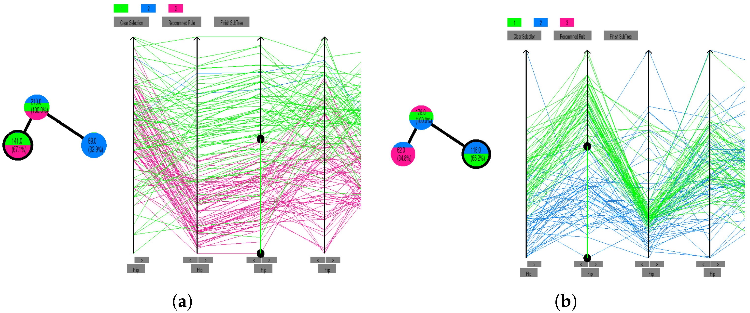
Figure 1. Two examples, each exploring a different dataset and focussing on different leaves. (a) Exploring the seed dataset. (b) Exploring the wine dataset.
Information 13 00464 g001
Figure 2. The types of splits that the user can apply to further a leaf to interactively refine a decision tree. Split (a) and split (b) are familiar from standard decision tree construction. However, a rectangular split (c) provides an excellent trade-off between interpretability and multivariate splits.
Information 13 00464 g002
Figure 3. The use of ML metrics of discrimination (in this case, both, information gain or gini ratio) sorts the attributes from left to right and elects the highlighted split. However, a human would chose a better (more purifying) split, such as the second attribute that isolates the blue class with a robust gap, or the fourth attribute, which isolates the brown class with also a wide gap. This situation illustrates how HITL-ML can deliver better models.
Information 13 00464 g003
Figure 4. Illustrations of the HITL-ML systems used for IML to build DTCs with either a high precision or high recall for the “black” class (coloured red). (a) High recall DTC. (b) High precision DTC.
Information 13 00464 g004
Figure 5. Example of how our HITL-ML system using parallel coordinates to visualise the decision path of a single leaf in a DTC.
Information 13 00464 g005
Figure 6. Disconnected sections on a single axis through negated split condensing rules. The green and negated red selections result in two selected ranges (third axis).
Information 13 00464 g006
Figure 7. Composition of DTC and HITL-ML survey for participants in Group A and Group B.
Information 13 00464 g007
Figure 8. Layout of survey for Experiment 1. The table on the right shows instances reaching the selected node. The class column colours instances with a distinctive colour for the class. The top instances show up as blue boxes on the table, the users would need to scroll down to find those instances belonging to the red class and to the green class.
Information 13 00464 g008
Figure 9. The layout of Experiment 2 for users in Group A (left) and Group B (right).
Information 13 00464 g009
Figure 10. Layout of survey section introducing DTC. When the leaf node is selected, the data table is updated to those exemplars that arrive to this node. Since most of them are from a class coloured red, the class column shows most of them have a red box in this column.
Information 13 00464 g010
Figure 11. Layout of survey section introducing PC.
Information 13 00464 g011
Figure 12. Layout of survey section introducing HITL-ML. The selection of the root node in the tree shows that there are three classes each with a different colour. The display on the right shows the exemplars of the three classes on the two attributes chosen by the user.
Information 13 00464 g012
Figure 13. Graph of distribution of response from Experiment 3.
Information 13 00464 g013
Table 1. Training set accuracy of each DTC presented to participants.
Tree No.DatasetAccuracy
1Wine69
2Wine99
3Wine90
4Cryotherapy72
5Cryotherapy92
6Seeds72
7Seeds95
8Seeds82
Table 2. Questions for Experiment 3.
Question No.Question
Q1Which system do you believe provides a better method of finding splits to build a decision tree classifier?
Q2Which system allows you to better navigate and understand the current state of a decision tree classifier as it is being constructed?
Q3Which system allows you to more easily determine how often a tree will predict the class correct class of an instance?
Q4Which system allows you to more easily find nodes in a decision tree classifier that need additional splits?
Q5Which system would provide better assistance to you when constructing a decision tree?
Q6Based on the videos you have seen, which system would you prefer to use to build a decision tree classifier?
Table 3. Results for Experiment 1.
GroupMean Accuracy DifferencesMean Accuracy Time (s)Mean RImp Mean Leaf Choice Time (s)
A17.8%80.20.25917.6
B19.0%49.30.28217.1
Table 4. Results for Experiment 2.
GroupMean AccuracyMean Time per Leaf (s)
A77.5%24.0
B86.7%6.7
Table 5. Results for Experiment 3.
QuestionQ1Q2Q3Q4Q5Q6
Strongly PC-based system384239445857
Somewhat PC-based system322732332526
Strongly UserClassifier776457
Somewhat UserClassifier2321211387
No differences4761087
Subtotal PC-based system706971778383
Subtotal UserClassifier302827171314
Publisher’s Note: MDPI stays neutral with regard to jurisdictional claims in published maps and institutional affiliations.